Three-Level Optimal Scheduling and Power Allocation Strategy for Power System Containing Wind-Storage Combined Unit

Nomenclature

1  Introduction

As a prominent renewable energy source, wind power is progressively integrating significantly into the grid, addressing both the energy crisis and environmental pollution [1,2]. Conventional scheduling models are ineffective for the power system integrating large-scale wind generation due to the inherent instability and restricted dispatchability of wind power [3]. Consequently, the effective mitigation of wind power’s fluctuation impact on the power grid has emerged as a central focus of global research efforts [4].

Due to its flexibility, energy storage technology has been widely used in peak shifting [5] and frequency modulation [6]. In addition, energy storage devices have the function of smoothing fluctuations, which can help to suppress power volatility [7,8]. The wind-storage hybrid system is an invaluable instrument for improving wind power’s dispatchability. However, one issue that needs to be taken into account in the optimal power system scheduling is how to synergistically enhance the output of both wind power and the energy storage system (ESS).

Optimal scheduling of the wind-storage combined systems has attracted much attention. The technique of using energy storage to support wind power scheduling is studied in the literature [9–11], which comprehensively considers the operation and optimization cycle cost of energy storage. Meanwhile, literature [12,13] optimize the allocation of energy storage capacity to enhance the wind-storage bundling scheduling capability. Considering large-scale wind power access’s high uncertainty and volatility, dual timescale coordination is used in the literature to adjust the energy storage output in response to actual wind power generation [14]. Similarly, literature [15] proposes a day-ahead optimal scheduling scheme of energy storage to mitigate wind energy instability. Although most of the literature has focused on wind-storage joint optimization, decisions on the charging and discharging intervals of energy storage have not yet been made from the perspective of fully exploiting the function of energy storage.

Many scholars view the wind farm as a whole as a wind power cluster (WPC) to fully utilize the complementarity and correlation of power output between wind farms (WFs) to smooth the overall production [16–18]. The optimal scheduling of WPC can be divided into two levels, including the scheduling of the system integrating WPC and the power allocation within the WPC. Since the active scheduling of wind-containing systems is a high-dimensional and complex problem, some studies have adopted different approaches to cope with the issue of dimensionality disaster. For example, literature [19] uses the Alternating Direction Method of Multipliers (ADMM) method to develop an active power optimal scheduling model within a wind farm (WF), and literature [20] proposes a distributed economic scheduling method for wind-containing systems. However, little literature has combined system-level optimal scheduling with wind-level power allocation to reduce wind power volatility and abandonment. This can coordinate the WPC and other units within the system, as well as the wind farm output within the WPC. In addition, some studies have used model predictive control strategies to track scheduling instructions in real-time due to the unavoidable errors in wind power forecasting [21,22]. On the other hand, literature [23,24] establish scheduling models using different timescales. Coordinating the allocation of wind energy on long and short timescales is an issue that deserves consideration.

Consequently, this paper proposes a multi-level optimization strategy for power scheduling and allocation in a power system containing the wind-storage combined unit. The specific contributions include: 1) Starting from the function of energy storage in smoothing power fluctuation and peak shaving-valley filling, the charging/discharging intervals of energy storage are set based on the day-ahead prediction data of the load and WPC. 2) It coordinates wind-storage output and the power allocation within WPC at both the system and wind power levels, with the primary goal of minimizing output variability. 3) The power allocation of WPC adopts a coordinated strategy containing both long- and short-term time scales. After obtaining the planned output of WFs on the long timescale, correct the output on the short timescale. It can maintain the tracking accuracy of the scheduling instruction while increasing wind power consumption and decreasing wind power volatility.

The other sections are arranged as follows: Section 2 describes the implementation process of the three-level optimal scheduling and power allocation strategy. Section 3 constructs the scheduling model of each level, including the objective function and constraints. Section 4 introduces the solution algorithms of the optimization model of each level and the corresponding algorithmic simplification. Section 5 verifies the effectiveness of the proposed strategy by analyzing the arithmetic examples. The last section gives the conclusions.

2  Framework for Three-Level Optimization Scheduling Strategy

The framework for the three-level optimization scheduling strategy, as depicted in Fig. 1, is driven by specific motivations. On the one hand, based on the scheduling sequence of the wind-containing system, we progressively optimize the power allocation from the system level to the WPC level. On the other hand, following energy conservation and environmental protection principles, we prioritize using clean and renewable energy sources, setting scheduling priorities in the order of wind-storage followed by thermal power.

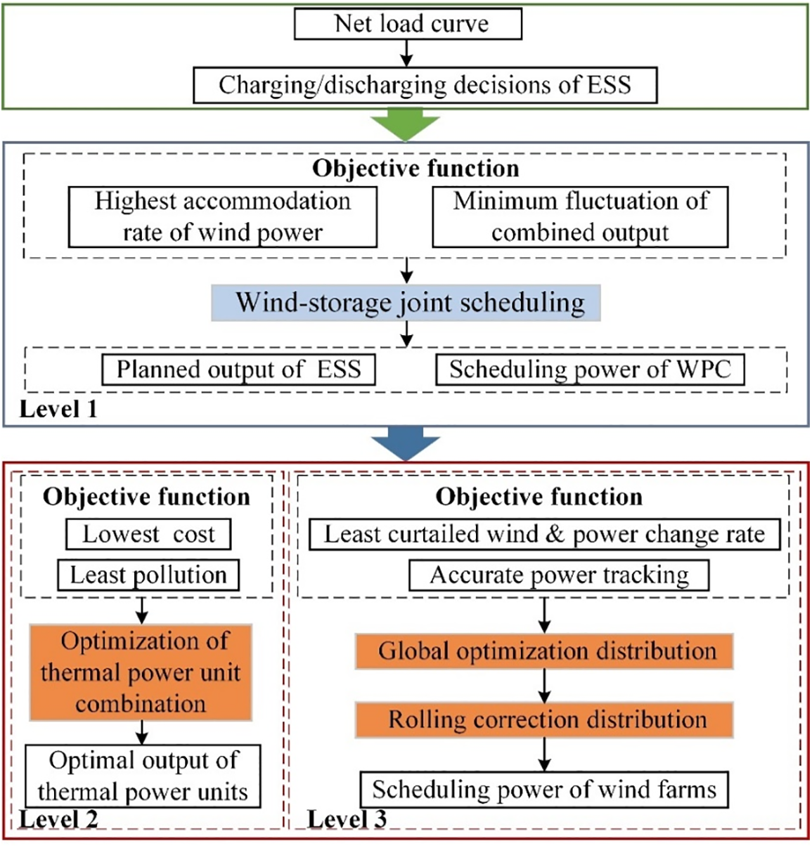
Figure 1: Framework for three-level collaborative optimization scheduling strategy

The first level is the wind-storage joint scheduling. It is developed from the perspective of wind power accommodation level and joint operation stability while considering the joint output of WPC and ESS as a stable schedulable power source. Then, the optimal production of the wind-storage joint scheduling is transmitted to the following levels. The second level is the combination of thermal power units. To balance the system’s operational efficiency with ecological sustainability, the optimization objective at this level is defined as minimizing the overall cost and reducing pollution emissions, thereby reasonably allocating the output of each unit. The third level performs the power allocation of WPC according to the wind power scheduling power at the first level, intending to maximize the wind energy utilization and minimize the output fluctuation. The specific scheduling process is as follows:

(1) According to the net load data, where the net load means the value of load minus the output of WPC, the states of ESS are decided. The wind-storage combined unit adopts the mixed integer linear programming (MILP) method to obtain the scheduling power of WPC and the planned output of ESS on the following day, where the time scale is 1 h.

(2) Calculate the net load again at each scheduling period, where the net load means the value of load minus the combined output of WPC and ESS. This value is subsequently applied to the system balance constraint. The next-day generation plan for the thermal power units is optimized using the MILP algorithm, with the same time scale as the first level.

(3) According to the scheduling power of WPC obtained from the optimization of the wind-storage combined unit, power allocation is carried out for WPC. To ensure the overall stability of the WFs in the coming day, carry out the power allocation firstly on a long timescale, i.e., 24/1 h. Then, refine the time scale and perform a rolling optimization of 1 h/15 min based on the value obtained from optimization on the long-time scale.

3  Scheduling Model for Power System Containing Wind-Storage Combined Unit

3.1 The First Level: Scheduling Model of Wind-Storage Combine Unit

3.1.1 Objective Function

The goal of this level is to reduce wind power abandonment, as well as the fluctuation of wind-storage combined output. The objective function is:

Fws=min[∑t=1TPtC+1T∑t=1T(PtWS−PaveWS)2](1)

{PtWS=PtW+PtSd−PtScPaveWS=1T∑t=1TPtWS(2)

where PtC, PtW are the amount of curtailed wind and output of WPC at time period t, respectively. PtWS denotes the wind-storage joint output, PtSd, PtSc are the discharging and charging power at time period t, respectively, T is the number of scheduling time periods.

3.1.2 Constraint Conditions

(1) WPC output constraint

PminW≤PtW≤PtWpre=PtWavi=PmaxW(3)

(2) Power balance equation constraint

PtWavi=PtW+PtSd−PtSc+PtC(4)

where PtC≥0. In order to avoid too much power generation from energy storage, which leads to unnecessary energy waste, wind power abandonment is set to be higher than 0 here.

(3) Charging/discharging state constraints

ItSd+ItSc≤1(5)

where ItSd is the discharging state, taking 1 for discharging and 0 for charging, ItSc is the discharging state, taking 1 for charging and 0 for discharging.

(4) Charging/discharging power constraints

ItSdPminSd≤PtSd≤ItSdPmaxSd(6)

ItScPminSc≤PtSc≤ItScPmaxSc(7)

(5) State of charge constraints

SOCt=SOCt−1+(PtScηc−PtSd/ηd)ΔT/SN(8)

SOCmin≤SOC≤SOCmax(9)

SOCT=SOC0(10)

where SOCt is the state of charge (SOC) of the ESS, SN is the rated capacity of the ESS, and ΔT is the scheduling interval.

3.2 The Second Level: Unit Combination Model for Thermal Power

3.2.1 Objective Function

This level is based on the first level’s optimization results, aiming to reduce operating and environmental costs and optimize unit combinations. The specific objective functions are as follows:

FEC=∑t=1T∑i=1NG[(ai(Pi,tG)2+bi(Pi,tG)+ci+Ci,tU(1−ui,t−1))ui,t](11)

FEV=∑t=1T∑i=1NG(αi+βi(Pi,tG)+γi(Pi,tG)2)ui,t(12)

where ai, bi, and ci are the coefficients of the consumption function, ui,t indicates the operating status, Ci,tU is the start-up cost for the thermal power unit, αi, βi, and γi are pollutant emission coefficients.

3.2.2 Constraint Conditions

(1) Power balance equation constraint

∑i=1NGPi,tG+PtWopt+PtSdopt−PtScopt=PtL(13)

where PtWopt, PtSdopt, PtScopt are the optimal solutions obtained from the wind-storage co-optimization; PtL denotes the load demand.

(2) Thermal power unit operating constraints

1) Power and its ramping constraints

ui,tPiGmin≤Pi,tG≤ui,tPiGmax(14)

2) Minimum start-stop time constraints

∑t′∈[t,t+Tiu]ui,t′≥Tiu⋅vi,t(15)

∑t′∈[t,t+Tid−1](1−ui,t′)≥Tid⋅wi,t(16)

ui,t−ui,t−1=vi,t−wi,t(17)

vi,t+wi,t≤1(18)

where Tiu, Tid refer to the minimum continuous operation and shutdown time of the thermal power unit i, the two Boolean variables vi,t and wi,t represent the start-up and shutdown actions.

3.3 The Third Level: Power Allocation for WPC

3.3.1 Objective Function

This level allocates power to each WF according to the WPC’s scheduling instructions issued by the wind-storage combined system. The scheduling power of WPC is optimized at the day-ahead time scale, aiming primarily to minimize wind power fluctuation while ensuring sufficient wind power accommodation. The objective function is established as follows:

FwGO=min[α1∑w=1NW(Pw,t+Δtopt−Pw,t+Δtpre)2+α2∑w=1NW(Pw,t+Δtopt−Pw,tact)2](19)

where Pw,t+Δtopt, Pw,t+Δtpre are the planned and predicted power of WF w at time period t + Δt, respectively, Pw,tact is the actual output of WF w at the sampling moment t, Δt is 1 h, NW is the number of WFs, α1, α2 are the weighting factors for the performance indicator, and set α1=0.2, α2=0.8.

Considering the roughness of the wind farms’ allocated output in the day-ahead scheduling timescale, the actual output is likely much smaller than the scheduling output at a certain moment, and the tracking effect is poor. Therefore, this level will refine the time scale and formulate the output of WFs within the short scheduling time scale on a rolling basis. The objective function is established as follows:

FwRO=min∑r=1R[∑w=1NW(Pw,t+Δtopt−Pw,t+rΔt1opt)2+∑w=1NW(Pw,t+rΔt1opt−Pw,t+rΔt1pre)2+(∑w=1NWPw,t+rΔt1opt−Pt+ΔtWopt)2](20)

where Pw,t+rΔt1opt, Pw,t+rΔt1pre are the planned and predicted output of WF w at time period t + rΔt1, respectively, Pt+ΔtWopt is the scheduling instruction issued to WPC by the system, i.e., the scheduling power of WPC obtained from the optimization of the wind-storage combined system, Δt1 is 15 min, r is the number of rolls.

3.3.2 Constraint Conditions

The constraints corresponding to the WPC power allocation problem on the long timescale for the first day are as follows:

(1) System scheduling plan constraints

∑w=1NWPw,t+Δtopt=Pt+ΔtWopt(21)

(2) Wind farm output constraints

Pw,t+Δtmin≤Pw,t+Δtopt≤Pw,t+Δtmax=Pw,t+Δtpre(22)

where Pw,t+Δtmax, Pw,t+Δtmin denote the upper and lower output of WF w.

(3) Wind farm ramping constraints

Pw,t+Δtopt−Pw,tact≤CwPwN(23)

where Cw denotes the ramping rate limit for WF w, PwN denotes the rated capacity of WF w.

Only wind power output and ramping constraints are included for the constraints on the WPC power allocation problem in the intraday time scale.

(1) Wind farm output constraints

Pw,t+rΔt1min≤Pw,t+rΔt1opt≤Pw,t+rΔt1max=Pw,t+rΔt1pre(24)

(2) Wind farm ramping constraints

Pw,t+rΔt1opt−Pw,t+(r−1)Δt1act≤CwPwN(25)

where Pw,t+(r−1)Δt1act denotes the actual value of WF w at moment t + (r−1)Δt1.

4  Model Solving

4.1 Linearization of Objective Function and Constraint Conditions

This paper linearizes the model containing nonlinear expressions such as 0–1 variables and square terms to convert it into a MILP model.

(1) Coal consumption and pollution emissions from the thermal power units

The consumption function of the thermal power units is generally expressed as the quadratic function of generation power, which is approximately transformed into a linear function by piecewise linearization, as shown in Fig. 2. Therefore, the linearized coal cost is expressed as:

F(Pi,tG)⋅ui,t=[F(PiGmin)+∑pl=1MKi,gl⋅δi,t(pl)]⋅ui,t∀i,∀t(26)

where F(PiGmin) is the consumption function corresponding to the unit i operating at the minimum output, i.e., F(PiGmin)=ai(PiGmin)2+bi(PiGmin)+ci, M is the number of linearized segments of the consumption characteristic curve; Ki,gl denotes the slope of unit i in the plth segment; and δi,t(pl) refers to the output power of unit i in the plth segment at time period t which is an added control variable that satisfies the following constraints:

0≤δi,t(pl)≤Di,gl−Di,gl−1∀i,∀t,∀gl(27)

where Di,gl refers to the glth segmentation point, and Di,0=PiGmin, Di,M=PiGmax.

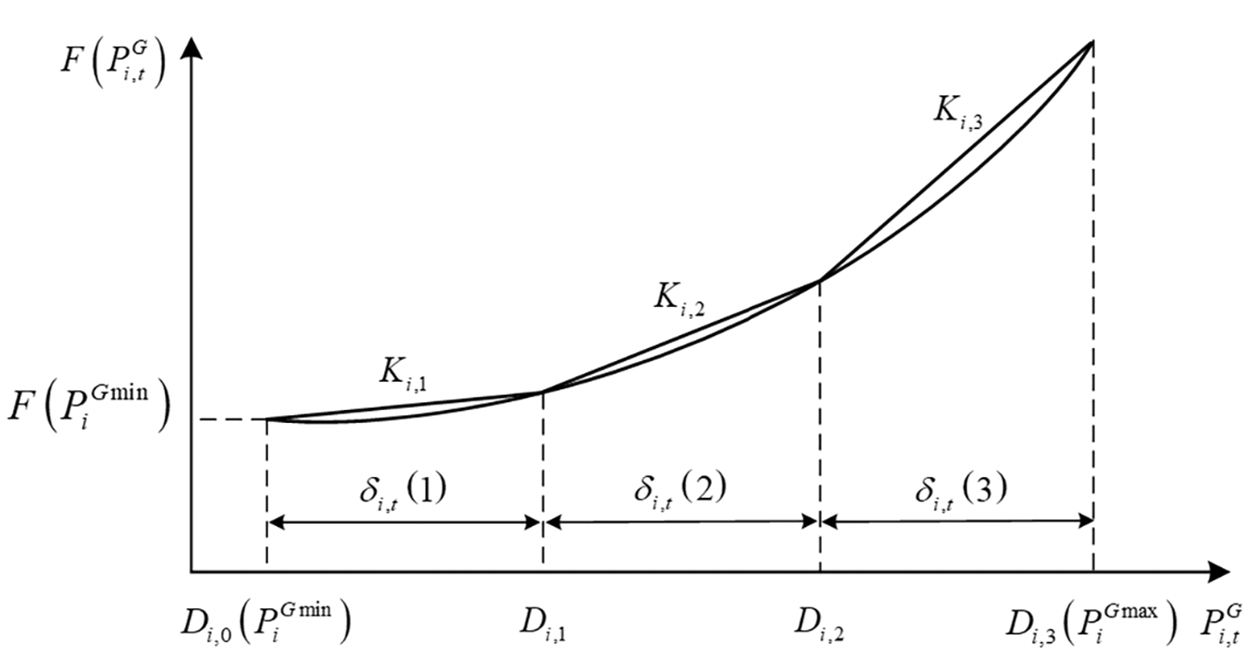
Figure 2: Piecewise linearization of coal consumption characteristics of thermal power units

Similarly, the pollution emission function is also linearized by segments, which will not be repeated here.

(2) Thermal power unit start-stop cost

The thermal power start-stop cost contains a nonlinear product term ui,tui,t−1, so an integer variable Ai,t is introduced instead. Let Ai,t=ui,tui,t−1, then the linearized start-stop cost expression is shown in Eq. (28), with Eq. (29) being the added linear constraint.

Ci,tUD(ui,t−Ai,t)(28)

{0≤Ai,t≤ui,tAi,t≤ui,t−1Ai,t≥ui,t+ui,t−1−1(29)

4.2 Charging and Discharging Decisions for Energy Storage

The average value μNL, the standard deviation σNL, the deviation ΔPtNL of the net load PtNL, and the deviation threshold δ are calculated as follows:

{PtNL=PtL−PtWμNL=1T∑t=1TPtNLσNL=1T∑t=1T(PtNL−μNL)2ΔPtNL=PtNL−μNLδ=min{PmaxESS,λσNL}(30)

where PmaxESS is the rated power of ESS, 0 < λ < 1.

To enhance the regulation performance of energy storage and maintain its continuous effectiveness during the scheduling period, determine the states of ESS based on its operating mode. The specific process, as shown in Fig. 3, involves two steps: smoothing power fluctuation, peak shaving and valley filling.

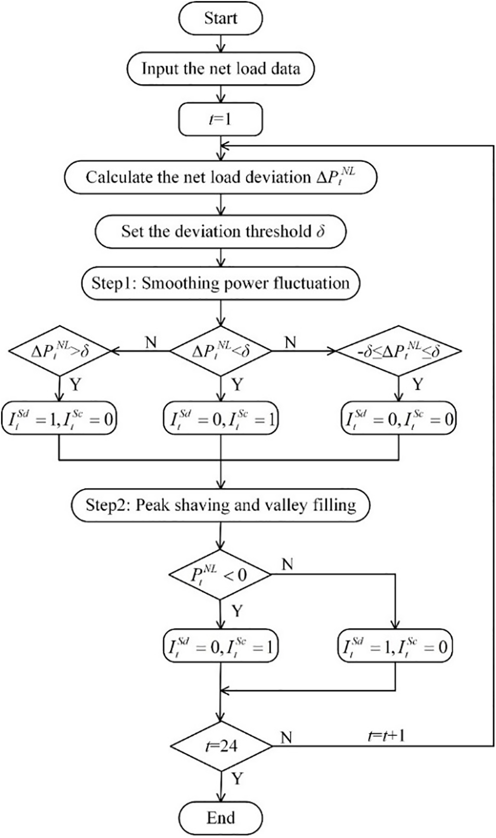
Figure 3: Flowchart of decision-making for the operating state of ESS

4.3 Rolling Optimization Correction for Wind Cluster Power Allocation

A rolling finite time domain optimization strategy is used for wind power allocation correction on a short time scale. According to the current performance index, the optimal control sequence within the finite time domain is determined. The real-time state of the system is re-sampled at the next moment, and the optimal control sequence continues to be solved. At each moment, the actual active power value of the WF is used as the initial value for a new round of rolling optimization scheduling to continue with rolling optimization at the next moment. The correction amount of the WF is selected as the control variable, i.e., ΔPw,t+rΔt1opt, the optimized WF’s scheduling value is:

Pw,t+rΔt1opt=Pw,tact+ΔPw,t+rΔt1opt(31)

where Pw,tact=Pw,t+Δtopt.

The steps for implementing the rolling optimization correction for wind cluster power allocation on a short time scale are specified below:

Step 1: At the current moment t + rΔt1, the actual values of each WF are initialized based on the planned values on a long-time scale scheduling;

Step 2: Update power predictions for WFs in a finite time domain based on the prediction model;

Step 3: The correction value in the control time domain of each WF is calculated according to Eq. (20), and the first column of control quantities is sent to each WF;

Step 4: Update the actual value of the WF at this moment;

Step 5: Return to Step 2 and solve for the power allocation value of the WF at the next moment, i.e., t + (r + 1)Δt1, until the optimization solution is completed for the whole optimization cycle.

5  Example Analysis

5.1 Basic Data and Parameters

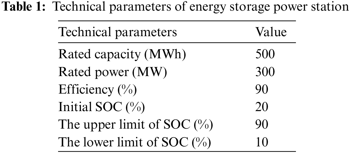
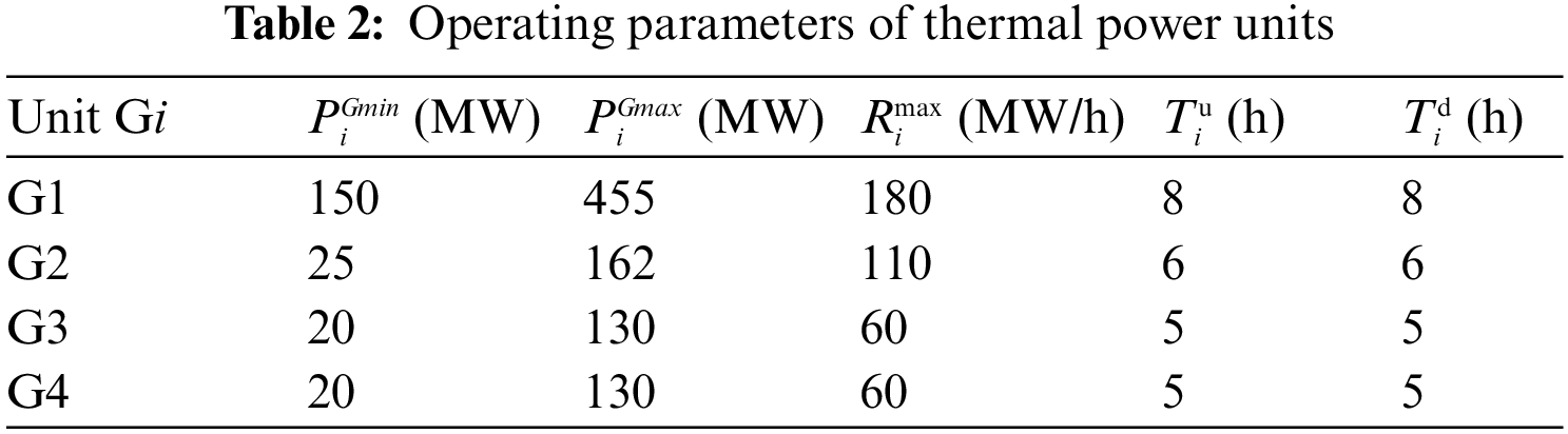
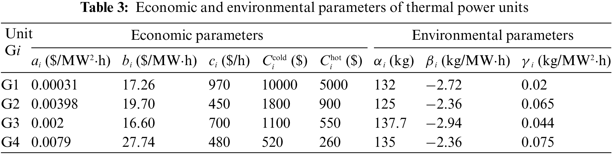
In this paper, a natural wind-storage-thermal combined system in China is used as an example for optimal scheduling and power allocation at the system level and cluster level, respectively. The example contains four thermal power units, three WFs, and one energy storage system, in which the rated capacities of WF1 and WF3 are both 400 MW, and that of WF2 is 300 MW. The day-ahead predicted outputs of WPC and load are shown in Fig. 4. The relevant parameters of the energy storage system and the thermal power units are shown in Tables 1–3.

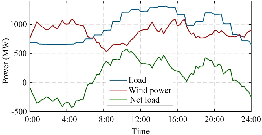
Figure 4: Day-ahead forecast data of load and WPC

5.2 Analysis of Scheduling Results with ESS Operating in Different Charging/Discharging Modes

To verify the effectiveness of the proposed energy storage charging/discharging decisions in this paper, set up two cases as follows:

Case 1: The charging/discharging states of ESS, together with the charging/discharging power of ESS and the scheduling power of WPC, are used as decision variables to optimize the solution.

Case 2: According to the net load forecast curve, with the purpose of peak shaving-valley filling and smoothing the wind power fluctuation, the charging/discharging states of ESS are decided. Only the scheduling power of ESS and WPC are optimally solved as decision variables.

Figs. 5–7 show the optimized scheduling results under the two cases, where (a) shows the optimized results for Case 1 and (b) shows the optimized results for Case 2. A comparative analysis of the scheduling results in Case 1 and Case 2 is presented in the following section.

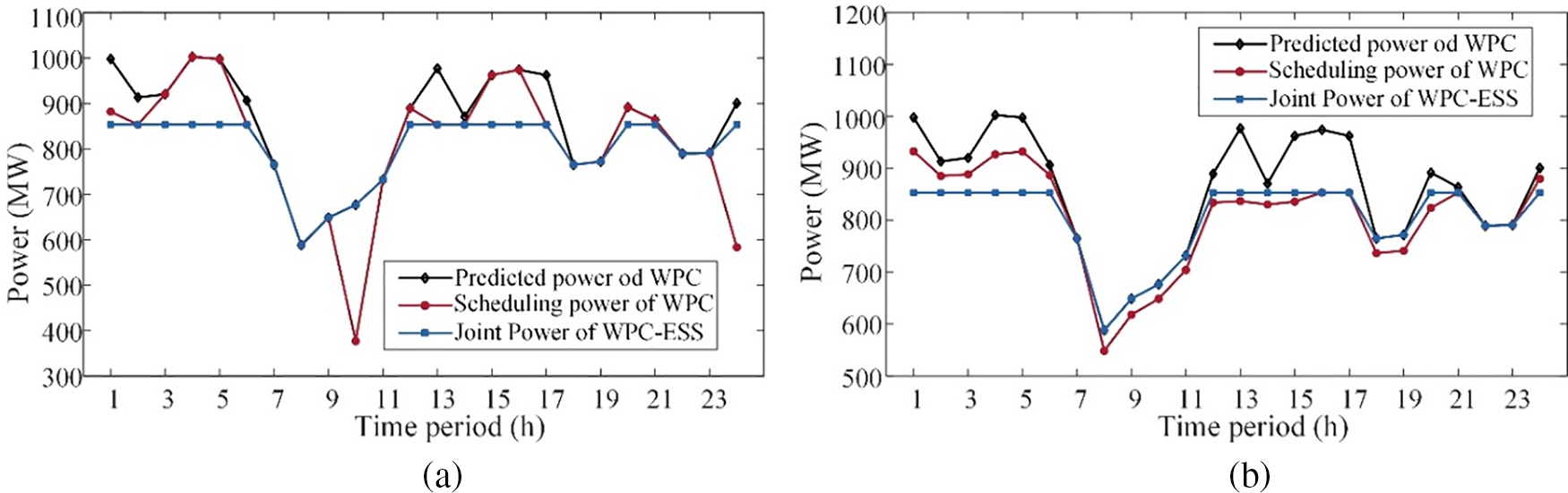
Figure 5: Scheduling power of WPC and ESS in (a) Case 1 and (b) Case 2

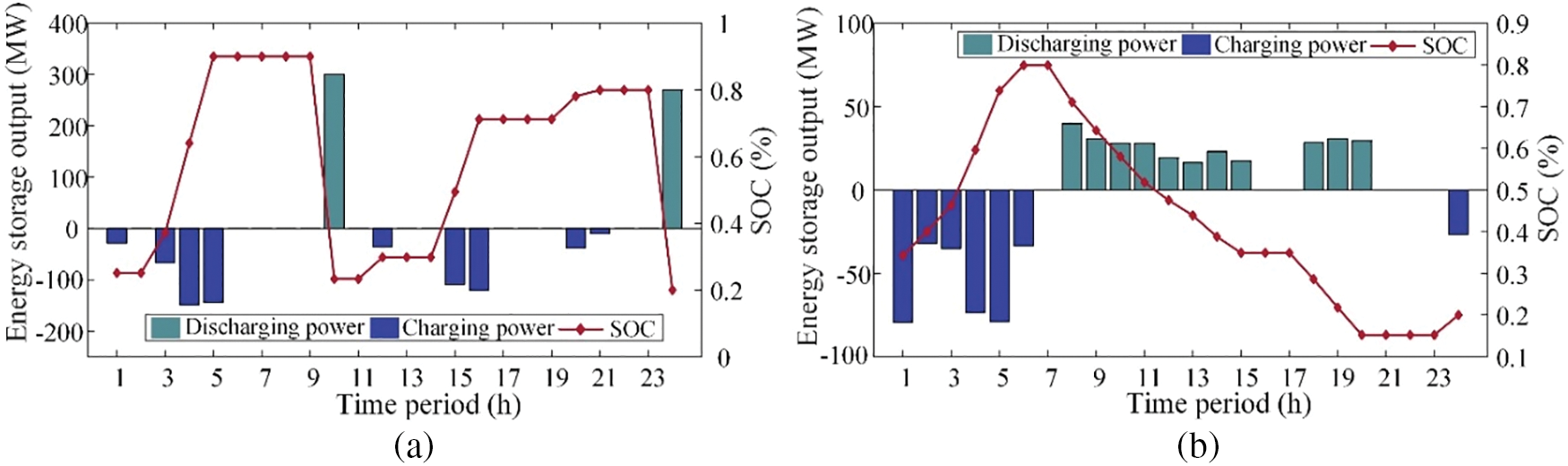
Figure 6: Operating state and optimal output of energy storage in (a) Case 1 and (b) Case 2

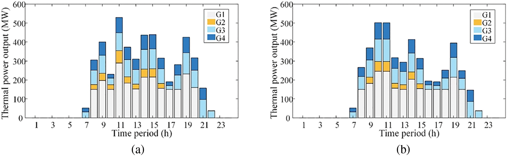
Figure 7: Optimal output of each thermal power unit in (a) Case 1 and (b) Case 2

Fig. 5 compares the day-ahead scheduling power of WPC for the two cases. In both cases, the optimized wind-storage combined power fluctuations are similar. However, it should be noted that the volatility of the scheduling power of WPC is lower in Case 2. Specifically, in Case 1, the scheduling power of WPC drops suddenly and sharply at time period 10, followed by a sharp increase at time period 11. In addition, the overall frequency of fluctuations in the scheduling curve of WPC is higher in Case 1. The sudden change in the reference power increases the complexity of power allocation at the WPC level. Therefore, the increased degree of scheduling power fluctuations of WPC may pose a threat to security and stability at both the system and the wind farm levels. In contrast, Case 2 effectively reduces the volatility of WPC’s scheduling power, thereby mitigating the negative impact of large-scale wind power access on the power system.

Fig. 6 shows the charging/discharging states and the charging/discharging power of ESS. In Case 1, to accommodate excess wind power, the ESS continues to charge at a high-power level during time periods 2–5 (i.e., the pre-load trough period). This results in subsequent periods being constrained by SOC and storage capacity, preventing the continuation of charging, which in turn leads to an increase in wind power volatility. In contrast, in Case 2, the ESS can maintain charging essentially throughout the load trough period, with storage capacity optimally allocated at time periods 1–7. Similarly, the ESS discharges to supply the load during the pre-peak load periods (e.g., time period 10 and time period 24) for peak shaving purposes in Case 1. However, only charging can be performed in subsequent periods due to excessive discharges in a short time. Furthermore, a comparison of the SOC in Cases 1 and 2 reveals that the SOC in Case 2 exhibits a more gradual change, while the SOC in Case 1 displays three distinct peaks and troughs. The frequency of charging/discharging of Case 1 in one scheduling cycle is also more significant than that of Case 2. This situation can harm the energy storage components and is not conducive to the long-term operation of ESS. Therefore, the charging/discharging decision of energy storage in Case 2 fully uses the peak shaving and power fluctuation smoothing effects of energy storage. This significantly reduces the degree of wind power fluctuation and slows down the ageing of the energy storage equipment while maintaining load balance.

Fig. 7 compares the thermal unit output in the two cases. It can be observed that in Case 2, the number of time periods when all thermal units are started at the same time is less than that in Case 1. The overall power output of thermal units is also lower in Case 2. Consequently, a reasonable energy storage charging/discharging strategy helps reduce the proportion of thermal power generation and the generation burden of thermal power units.

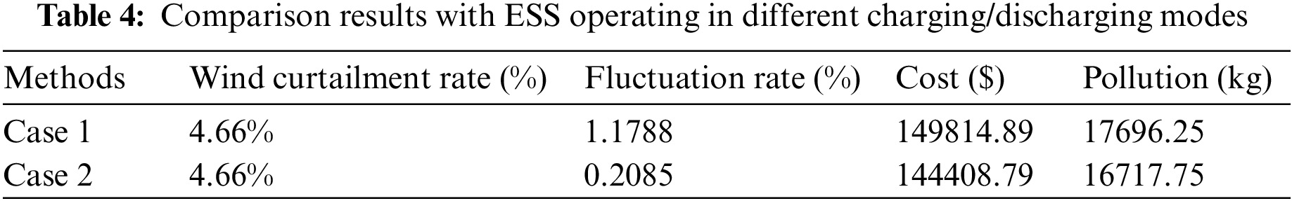
To compare the optimization results of Case 1 and Case 2 more comprehensively, we compared their average wind curtailment rate, wind power fluctuation rate, economic cost, and amount of pollution, as shown in Table 4. Although the wind curtailment rate is the same in both cases, the wind power fluctuation rate, unit generation cost, and pollution amount are significantly lower in Case 2. It can be seen that the proposed strategy, under the premise of ensuring safe and stable operation of the system, can take into account the economy and environmental protection of the joint system.

5.3 Analysis of Scheduling Results for WPC in Different Power Allocation Methods

The superiority of Case 2 has been verified in the previous subsection so that WPC will perform power allocation according to the scheduling power in Case 2. To verify the effectiveness of the proposed power allocation strategy, compare the global optimization allocation (GOA) strategy with the traditional fixed proportional allocation (FPA) strategy and variable proportional allocation (VPA) strategy first. The scheduling power of each WF under the three power allocation strategies is shown in Fig. 8, where the dotted line indicates the day-ahead predicted power of each WF.

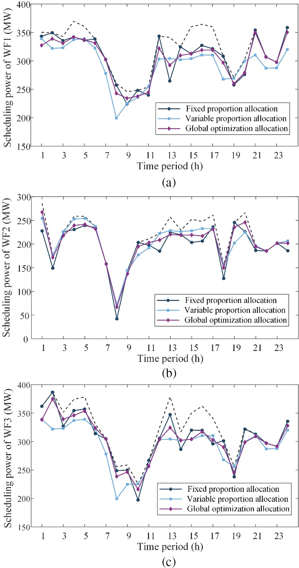
Figure 8: Scheduling output of wind farms under different allocation strategies. (a) WF1. (b) WF2. (c) WF3

This paper quantifies the amount of wind curtailment and the degree of fluctuation of each WF in the WPC power allocation phase. Table 5 shows each WF’s fluctuation and curtailment rates under different strategies.

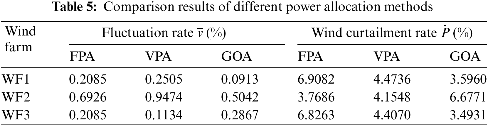
The two indicators are weighted in this paper to measure them integrated, and the specific mathematical expression is shown in Eq. (32).

Φ=α1v¯+α2P˙(32)

By calculating the above equation, we can get the values of comprehensive performance indexes under FPA, VPA, and GOA strategies, which are 2.7490, 2.4937, and 2.1706, respectively.

As seen from Fig. 8 and Table 5, the FPA strategy allocates power according to the proportion of unit capacity, and its overall active distribution effect is inferior to the other two strategies. It does not consider the forecast information, which may lead to larger wind power output and smaller scheduled power at some time periods, thus leading to an increase in wind curtailment in WFs. WF1 has a high output state at time periods 14–16. However, it has the largest wind curtailment amount when adopting the FPA strategy. The VPA strategy considers the forecast information, and its wind curtailment is reduced to some extent. Nevertheless, the power allocation does not consider the reduction of the volatility of wind power, which may result in a more significant change rate of wind power than the other two strategies. Overall, it can be seen that the scheduling power curves under the GOA strategy are basically between the scheduling power curves under the FPA and VPA strategies. This can avoid the shortcomings of the FPA and VPA strategies and take into account the two objectives of maximizing the utilization rate and minimizing the volatility rate of wind power. While some WFs using the GOA strategy may exhibit a higher wind curtailment rate or a greater power variation than those employing the other two strategies, the GOA strategy still demonstrates the smallest combined performance indicators among the three strategies.

Since the wind power allocation on a long timescale is rough, this paper corrects the allocated power of each WF on a short timescale. The corrected scheduling power of each WF is shown in Fig. 9.

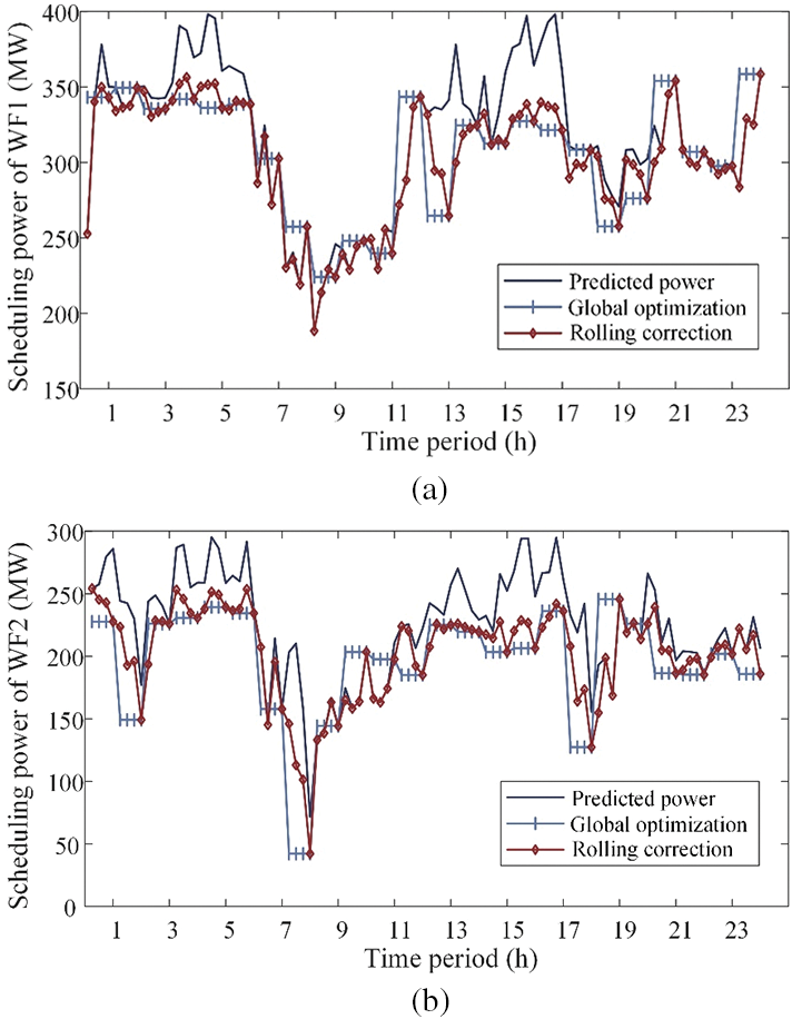
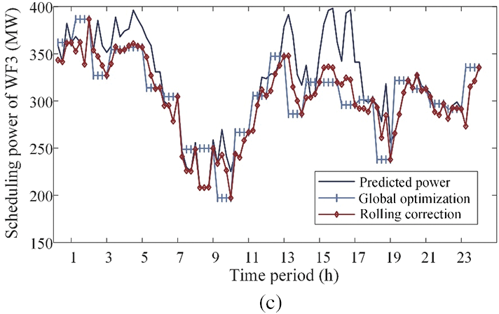
Figure 9: Scheduling output of wind farms on long- and short-time scales. (a) WF1. (b) WF2. (c) WF3

To further evaluate the role of rolling correction in the power allocation of WPC, this paper compares the average wind curtailment rate and power tracking accuracy after global optimization and rolling correction of WPC. The corresponding values are given in Table 6. The average mean relative error (AMRE) is taken as the tracking performance index to measure the power tracking accuracy, and its index calculation formula is:

ηAMSE=1M∑m=1M|∑w=1NwPw,mopt−PmW|(33)

where M is the total scheduling time period, Pw,mopt is the scheduling power of WF w at time period m, and PmW is the value of the scheduling power of WPC issued by the system.

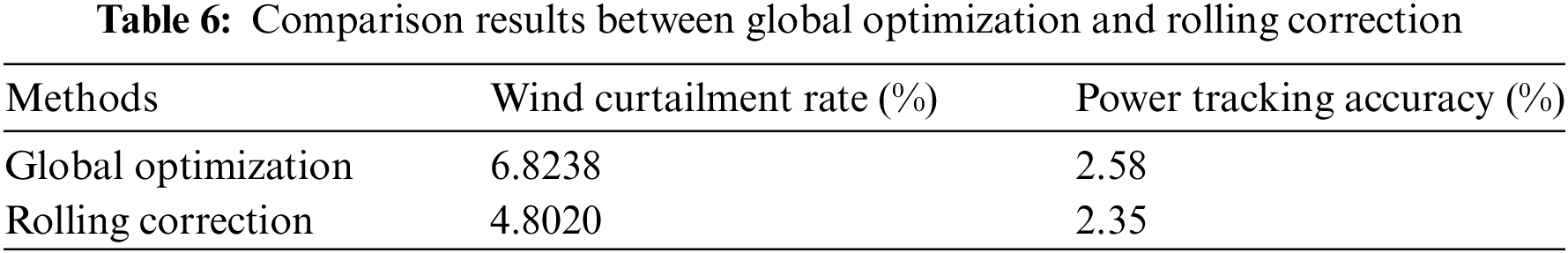
The power scheduling curves in Fig. 9 show that during the global optimal allocation of WPC, there are occasional instances where the WF’s generatable capacity is less than the scheduling power. This may result in the WF being unable to track the scheduling instructions issued by the system accurately. This situation primarily results from the inaccurate forecasts of wind power and the stochastic nature of wind power. Moreover, the scheduling power optimized globally can be corrected in a rolling manner on a more detailed time scale by updating the data in real-time. In addition, this can make the planned scheduling curve of the WF lie on top of the globally optimized scheduling curve, further dissipating wind power and reducing the waste of resources. The comparison of values in Table 6 further validates the necessity of short-time correction of power allocation. The wind curtailment rate is significantly reduced at this stage, while wind power tracking accuracy is enhanced.

6  Conclusions

Wind power is gradually moving towards high penetration into the grid, posing a significant threat to the power system due to its volatility. Therefore, this paper aims primarily at mitigating the volatility of wind power output by proposing a three-level coordinated optimal scheduling and power allocation strategy. The effectiveness of the proposed strategy is validated through case analysis, leading to the following conclusions:

(1)   As a flexible resource, energy storage can be combined with wind power to improve its dispatchability and stability. At the same time, the peak shaving-valley filling and fluctuation smoothing characteristics of ESS can be brought into full play by optimizing its charging and discharging intervals.

(2)   The designed power allocation strategy of WPC can take into account wind power smoothing and wind energy accommodation, thus avoiding the phenomenon of wind curtailment that may occur under the FPA strategy and the phenomenon of significant power fluctuation that may occur under the VPA strategy. Furthermore, the refinement of the scheduling time scale can reduce the tracking deviation of scheduling instructions of WFs, thereby improving the feasibility of issuing scheduling instructions.

(3)   This paper employs a level-by-level optimization strategy, issuing optimization scheduling instructions at each level. Wind-storage co-optimization is the first level of the optimization process, coordinating the outputs of wind power and energy storage. The second optimization level, namely the thermal power unit combination, considers the system’s overall economic and environmental benefits. Furthermore, the power allocation stage of WPC continues to pursue the objective of minimizing power fluctuation at the initial level. This approach considers the system’s stability, economic efficiency, and environmental protection as an integrated whole.

Acknowledgement: Sincere thanks are due to Professor Ying Zhu of Hohai University for providing lots of constructive suggestions.

Funding Statement: This work is supported by the State Grid Jiangsu Electric Power Co., Ltd. Technology Project (J2023035).

Author Contributions: The authors confirm contribution to the paper as follows: study conception and design: Jingjing Bai, Yunpeng Cheng; data collection: Fan Wu, Cheng Chen; analysis and interpretation of results: Jingjing Bai, Yunpeng Cheng, Shenyun Yao; draft manuscript preparation: Shenyun Yao, Fan Wu, Cheng Chen. All authors reviewed the results and approved the final version of the manuscript.

Availability of Data and Materials: Data available within the article.

Ethics Approval: Not applicable.

Conflicts of Interest: The authors declare that they have no conflicts of interest to report regarding the present study.

References

1. A. A. Eladl et al., “A comprehensive review on wind power spillage: Reasons, minimization techniques, real applications, challenges, and future trends,” Electr. Power Syst. Res., vol. 226, Jan. 2024, Art. no. 109915. doi: 10.1016/j.epsr.2023.109915. [Google Scholar] [CrossRef]

2. V. V. Yadav and B. Saravanan, “Technical advances and stability analysis in wind-penetrated power generation systems-A review,” Front. Energy Res., vol. 10, Dec. 2022, Art. no. 1091512. doi: 10.3389/fenrg.2022.1091512. [Google Scholar] [CrossRef]

3. L. L. Li, J. R. Pei, and Q. Shen, “A review of research on dynamic and static economic dispatching of hybrid wind-thermal power microgrids,” Energies, vol. 16, no. 10, May 2023, Art. no. 3985. doi: 10.3390/en16103985. [Google Scholar] [CrossRef]

4. S. G. Qin and D. S. Liu, “Distribution characteristics of wind speed relative volatility and its influence on output power,” J. Mar. Sci. Eng., vol. 11, no. 5, May 2023, Art. no. 0967. doi: 10.3390/jmse11050967. [Google Scholar] [CrossRef]

5. J. Liu, H. Y. Wang, Y. P. Du, Y. L. Lu, and Z. H. Wang, “Multi-objective optimal peak load shaving strategy using coordinated scheduling of EVs and BESS with adoption of MORBHPSO,” J. Energy Storage, vol. 64, Aug. 2023, Art. no. 107121. doi: 10.1016/j.est.2023.107121. [Google Scholar] [CrossRef]

6. C. P. Li, C. S. Feng, J. H. Li, D. C. Hu, and X. X. Zhu, “Comprehensive frequency regulation control strategy of thermal power generating unit and ESS considering flexible load simultaneously participating in AGC,” J. Energy Storage, vol. 58, Feb. 2023, Art. no. 106394. doi: 10.1016/j.est.2022.106394. [Google Scholar] [CrossRef]

7. T. Guo, Y. Zhu, Y. Liu, C. Gu, and J. Liu, “Two-stage optimal MPC for hybrid energy storage operation to enable smooth wind power integration,” IET Renew. Power Gener., vol. 14, no. 13, pp. 2477–2486, Oct. 2020. doi: 10.1049/iet-rpg.2019.1178. [Google Scholar] [CrossRef]

8. Y. Lv, R. Qin, H. Sun, Z. Guo, F. Fang and Y. Niu, “Research on energy storage allocation strategy considering smoothing the fluctuation of renewable energy,” Front. Energy Res., vol. 11, Mar. 2023, Art. no. 1094970. doi: 10.3389/fenrg.2023.1094970. [Google Scholar] [CrossRef]

9. A. Azizivahed et al., “Risk-oriented multi-area economic dispatch solution with high penetration of wind power generation and compressed air energy storage system,” IEEE Trans. Sustain. Energy., vol. 11, no. 3, pp. 1569–1578, Jul. 2020. doi: 10.1109/TSTE.2019.2931670. [Google Scholar] [CrossRef]

10. P. Roy, Y. Liao, and J. He, “Economic dispatch for grid-connected wind power with battery-supercapacitor hybrid energy storage system,” IEEE Trans. Ind. Appl., vol. 59, no. 1, pp. 1118–1128, Jan. 2023. doi: 10.1109/TIA.2022.3203663. [Google Scholar] [CrossRef]

11. S. Tampakakis and D. Zafirakis, “On the value of emerging, day-ahead market related wind-storage narratives in greece: An early empirical analysis,” Energies, vol. 16, no. 8, Apr. 2023, Art. no. 3506. doi: 10.3390/en16083506. [Google Scholar] [CrossRef]

12. M. Zhu et al., “The value of energy storage in facilitating renewables: A northeast area analysis,” Processes, vol. 11, Dec. 2023, Art. no. 3449. doi: 10.3390/pr11123449. [Google Scholar] [CrossRef]

13. J. Li, Z. Fang, Q. Wang, M. Zhang, Y. Li and W. Zhang, “Optimal operation with dynamic partitioning strategy for centralized shared energy storage station with integration of large-scale renewable energy,” J. Mod. Power Syst. Clean Energy, vol. 12, no. 2, pp. 359–370, Mar. 2024. doi: 10.35833/MPCE.2023.000345. [Google Scholar] [CrossRef]

14. Z. Guo, W. Wei, M. Shahidehpour, L. Chen, and S. Mei, “Two-timescale dynamic energy and reserve dispatch with wind power and energy storage,” IEEE Trans. Sustain. Energy., vol. 14, no. 1, pp. 490–503, Jan. 2023. doi: 10.1109/TSTE.2022.3217173. [Google Scholar] [CrossRef]

15. C. Wu, Q. Wu, and Q. Wu, “Robust day-ahead dispatch of CAES for mitigating fluctuation of net load in the distribution network,” IET Renew. Power Gener., vol. 14, no. 19, pp. 4104–4111, Dec. 2020. doi: 10.1049/iet-rpg.2019.1168. [Google Scholar] [CrossRef]

16. H. Chen, “Cluster-based ensemble learning for wind power modeling from meteorological wind data,” Renew Sustain. Energy Rev., vol. 167, Oct. 2022, Art. no. 112652. doi: 10.1016/j.rser.2022.112652. [Google Scholar] [CrossRef]

17. Z. Lin, Z. Chen, C. Qu, Y. Guo, J. Liu and Q. Wu, “A hierarchical clustering-based optimization strategy for active power dispatch of large-scale wind farm,” Int. J. Electr. Power Energy Syst., vol. 121, Oct. 2020, Art. no. 106155. doi: 10.1016/j.ijepes.2020.106155. [Google Scholar] [CrossRef]

18. J. Zhang et al., “Power prediction of a wind farm cluster based on spatiotemporal correlations,” Appl. Energy., vol. 302, Nov. 2021, Art. no. 117568. doi: 10.1016/j.apenergy.2021.117568. [Google Scholar] [CrossRef]

19. P. Hong and Z. Qin, “Distributed active power optimal dispatching of wind farm cluster considering wind power uncertainty,” Energies, vol. 15, no. 7, Apr. 2022, Art. no. 2706. doi: 10.3390/en15072706. [Google Scholar] [CrossRef]

20. P. Li, M. Yang, and Q. Wu, “Confidence interval based distributionally robust real-time economic dispatch approach considering wind power accommodation risk,” IEEE Trans. Sustain. Energy., vol. 12, no. 1, pp. 58–69, Jan. 2021. doi: 10.1109/TSTE.2020.2978634. [Google Scholar] [CrossRef]

21. J. Zhao et al., “Optimal scheduling strategy of wind farm active power based on distributed model predictive control,” Processes, vol. 11, Nov. 2023, Art. no. 3072. doi: 10.3390/pr11113072. [Google Scholar] [CrossRef]

22. L. Ye et al., “Hierarchical model predictive control strategy based on dynamic active power dispatch for wind power cluster integration,” IEEE Trans. Power Syst., vol. 34, no. 6, pp. 4617–4629, Nov. 2019. doi: 10.1109/TPWRS.2019.2914277. [Google Scholar] [CrossRef]

23. Y. Song and L. Shi, “Dynamic economic dispatch with CHP and wind power considering different time scales,” IEEE Trans. Ind. Appl., vol. 58, no. 5, pp. 5734–5746, Sep. 2022. doi: 10.1109/TIA.2022.3188603. [Google Scholar] [CrossRef]

24. J. Xu et al., “A multi-time scale tie-line energy and reserve allocation model considering wind power uncertainties for multi-area systems,” CSEE J. Power Energy Syst., vol. 7, no. 4, pp. 677–687, Jul. 2021. doi: 10.17775/cseejpes.2020.00620. [Google Scholar] [CrossRef]