
 Submit a Paper
 Propose a Special lssue
 Open Access
ARTICLE

Hydraulic Fracture Parameter Inversion Method for Shale Gas Wells Based on Transient Pressure-Drop Analysis during Hydraulic Fracturing Shut-in Period
1 Sichuan Changning Natural Gas Development Company, Chengdu, 610000, China
2 National Key Laboratory of Oil and Gas Reservoir Geology and Exploitation, Southwest Petroleum University, Chengdu, 610500, China
* Corresponding Author: Luqi Qin. Email:
Energy Engineering 2024, 121(11), 3305-3329. https://doi.org/10.32604/ee.2024.053622
Received 06 May 2024; Accepted 27 July 2024; Issue published 21 October 2024
 View Full Text
 Download PDF
Abstract
Horizontal well drilling and multi-stage hydraulic fracturing are key technologies for the development of shale gas reservoirs. Instantaneous acquisition of hydraulic fracture parameters is crucial for evaluating fracturing effectiveness, optimizing processes, and predicting gas productivity. This paper establishes a transient flow model for shale gas wells based on the boundary element method, achieving the characterization of stimulated reservoir volume for a single stage. By integrating pressure monitoring data following the pumping shut-in period of hydraulic fracturing for well testing interpretation, a workflow for inverting fracture parameters of shale gas wells is established. This new method eliminates the need for prolonged production testing and can interpret parameters of individual hydraulic fracture segments, offering significant advantages over the conventional pressure transient analysis method. The practical application of this methodology was conducted on 10 shale gas wells within the Changning shale gas block of Sichuan, China. The results show a high correlation between the interpreted single-stage total length and surface area of hydraulic fractures and the outcomes of gas production profile tests. Additionally, significant correlations are observed between these parameters and cluster number, horizontal stress difference, and natural fracture density. This demonstrates the effectiveness of the proposed fracture parameter inversion method and the feasibility of field application. The findings of this study aim to provide solutions and references for the inversion of fracture parameters in shale gas wells.Keywords
Nomenclature
| p | Pressure, Pa |
| xF | Hydraulic fracture half-length, m |
| wF | Hydraulic fracture width, m |
| h | Reservoir thickness, m |
| T | Reservoir temperature, K |
| q | Production rate, m3/s |
| k | Permeability, m2 |
| ϕ | Porosity, dimensionless |
| c | Composite compressibility coefficient, Pa−1 |
| μ | Viscosity, Pa·s |
| γ | Permeability modulus of the fracture, Pa·s/Pa2 |
| C | Well storage coefficient, m3·Pa |
| α | Matrix block shape factor, m−2 |
| s | Laplace transform variable |
| Storage ratio, dimensionless | |
| Transmissibility coefficient, dimensionless | |
| M | Ratio of permeability between outer and inner regions |
| The ratio of transmissibility coefficient between outer and inner regions | |
| Wi | Number of discrete hydraulic fractures in the i-th inner region |
| Si, j | Length of the j-th segment of hydraulic fracture in the i-th inner region |
| The flow rate of the j-th segment of hydraulic fracture in the i-th inner region | |
| δ() | Dirac function |
| xi, j, yi, j | The position of the j-th hydraulic fracture segment in the i-th internal zone |
| The normal vector of the boundary | |
| K0() | The zeroth-order Bessel function |
| ln | The dimensionless length of the nth discretized boundary segment |
| The dimensionless pressure of the j-th segment of hydraulic fractures in the i-th internal region | |
| τ | The ratio of the outer region to the hydraulic fracture conductivity coefficient |
| LDi, n | The dimensionless distance from the horizontal well to the n-th segment of the hydraulic fracture in the i-th internal region |
| Sk | Skin factor, dimensionless |
Horizontal wells with segmented multi-cluster hydraulic fracturing is the key technique to achieving effective development of shale gas reservoirs [1,2]. As crucial parameters for assessing fracturing efficiency, acquiring hydraulic fracture parameters is indispensable for predicting the Estimated ultimate recovery (EUR) of gas wells and evaluating the primary controlling factors affecting gas well productivity.
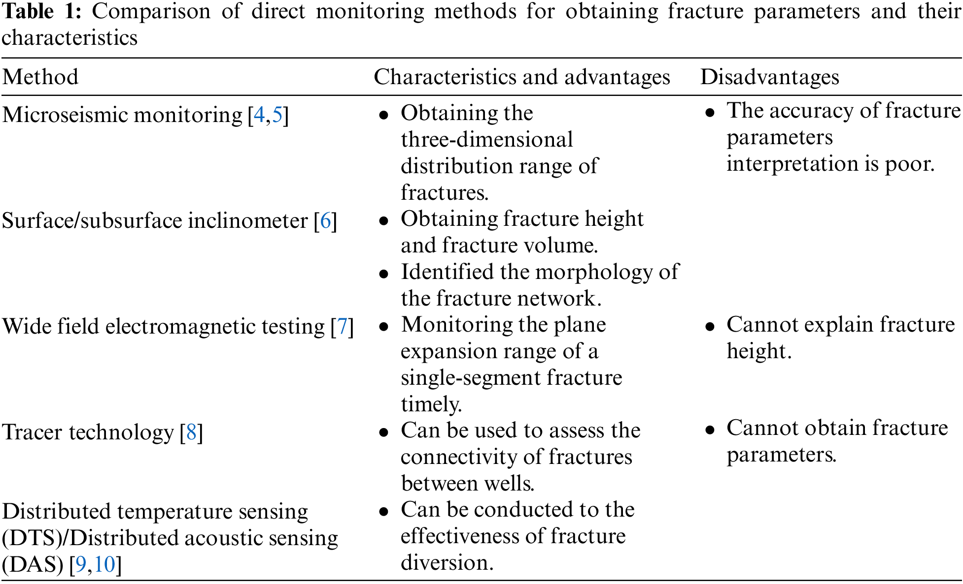
Currently, methods for obtaining hydraulic fracture parameters primarily fall into two categories: direct monitoring methods (as shown in Table 1) and indirect methods (as shown in Table 2) [3]. Direct monitoring methods provide intuitive results and have high confidence levels [4–6]. However, direct monitoring methods are generally costly, and achieving measurements for each well of gas field can be challenging [7–10]. To achieve large-scale batch inversion of hydraulic fracture parameters, opting for reliable indirect monitoring methods is highly appealing.
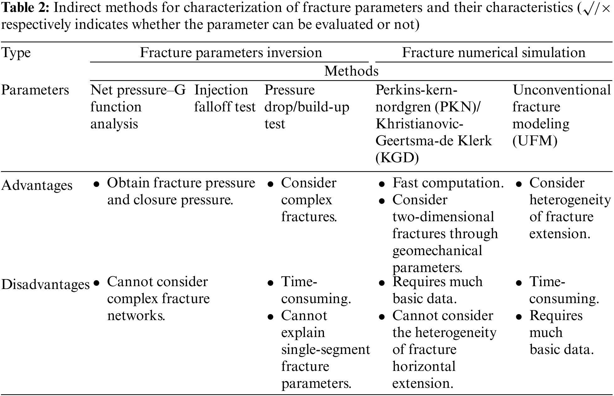
Indirect methods primarily rely on constructing numerical simulation models or transient seepage models. By adjusting model parameters, these methods aim to achieve a close fit between measured production data and calculated model data, ultimately obtaining fracture parameters. The indirect methods primarily include hydraulic fracturing simulation and inversion methods. Fracturing simulation relies heavily on accurate geological and geomechanical modeling [11–14], demanding many basic parameters. Moreover, the simulation process is time-consuming and may not meet the demand for rapid evaluation of fracturing effectiveness in the field [15,16]. Additionally, for shale gas reservoirs, the simulation results of hydraulic fractures are significantly influenced by the parameters of natural fractures. Obtaining these parameters accurately poses challenges, leading to uncertainties in the results of fracturing simulations.
Fracture parameters inversion methods include net pressure-G function analysis method [17], injection fall-off tests [18], and pressure drop/build-up well test analysis. The net pressure-G function analysis and injection fall-off tests assume that the hydraulic fracture is ideally a simple double-wing fracture shape, which cannot adequately characterize the complex fractures of shale gas wells. These two techniques are primarily applied in pre-fracturing experiments to predict breakdown pressure and closure pressure. The conventional well-testing analysis method involves pressure drop/build-up tests, utilizing analytical or semi-analytical well-testing models for typical curve fitting [19–23].
However, due to the extremely low permeability of the shale matrix, long-time pressure build-up tests are required. Furthermore, interpretation results provide average fracture parameters for each section of the entire well, which may not be conducive to interpreting volume hydraulic fractured shale gas wells, especially those with long horizontal sections.
For these issues, many scholars have explored alternative indirect methods for evaluating the effectiveness of hydraulic fracturing. In recent years, some researches have proposed the inversion of fracture parameters based on hydraulic fracturing curve analysis. Iriarte et al. [24] and Dung et al. [25] assessed fracture parameters through the analysis of the water hammer oscillation period and frequency during the pumping shut-in stage. However, the method offers only qualitative assessment and cannot quantitatively calculate the fracture parameters. Then, Liu et al. [26] developed an analytical formula based on the flow material balance theory to quantify the fracture surface area and the complexity of secondary fractures, which realized the quantitative interpretation of hydraulic fracture parameters of horizontal wells. However, this method necessitates the fracture height as an input parameter, making it impossible to determine both the fracture height and length simultaneously. Additionally, clear characteristics of the log-log curve of the pumping pressure-time are essential for their method, imposing relatively strict application conditions. Tompkins et al. [27] also present a new method for test design and analysis of diagnostic fracture-injection/falloff tests conducted in under pressured reservoirs. From these studies, we can glean an important insight: by utilizing pumping shut-in pressure-drop data in conjunction with well testing analysis, quantitative interpretation of single-stage fracture parameters can be achieved in hydraulically fractured wells. This approach offers the advantages of easy acquisition of basic data and high interpretation efficiency. However, existing studies have not fully developed a methodology for integrating shut-in pressure-drop data with well-testing analysis. To address this, the following issues need to be resolved: the well-testing model needs to accurately characterize the stimulated reservoir volume (SRV) for individual fracture stages, and effective measures are required to eliminate the challenge of generating well-testing type curve plots due to water hammer oscillations caused by rapid shut-in.
Based on this, this paper establishes a semi-analytical transient seepage model based on the multi-connected region boundary element method, which enables the characterization of irregular shapes in the SRV of single stage and the representation of heterogeneity in property parameters. Furthermore, by integrating pumping shut-in pressure drop data from single hydraulic fracturing stages of shale gas wells for well testing interpretation, and a corresponding workflow is constructed. Compared with existing fracture parameter inversion methods, the main contribution of this work is the inversion of single-stage fracture parameters in shale gas wells, rather than a general interpretation of the average fracture parameters for all stages of the well. Additionally, this method utilizes shut-in pressure decline data from fracturing operations, eliminating the need for additional production testing and thereby maximizing efficiency. The practical application of this methodology was conducted on 10 shale gas wells within the Changning shale gas block of Sichuan, China. The single stage hydraulic fracture parameters for each well are obtained, and conduct analysis of the correlations among productivity, stimulation parameters, geomechanically properties, and hydraulic fracture parameters. The finding of this study can serve as a valuable reference for the evaluation of hydraulic fracture parameters in shale gas wells.
2.1 Pre-Processing Pump Shut-in Pressure Data
The method for inversion of fracture parameters based on the hydraulic fracturing curve has been proven to be an efficient method. It includes two stages, where Stage I denotes the progress of fracture network extension and Stage II indicates pumping shut-in and leak-off (Fig. 1). In this paper, we select the pressure data from Stage II for pressure-drop analysis, however, pre-processing of the data is necessary to fulfill the requirements of well testing interpretation.
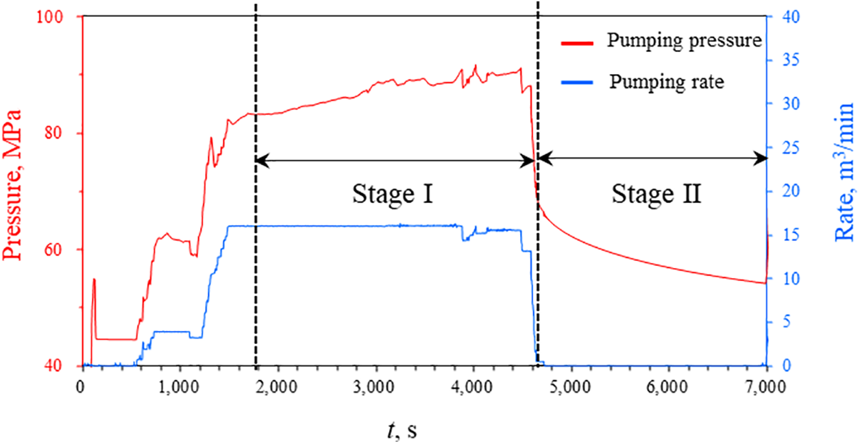
Figure 1: Fracturing curve and pressure-drop data of pumping shut-in stage
2.2 Bottom-Hole Pressure Conversion
During the initial period of pumping shut-in stage, fracturing fluid continues to flow within the wellbore, and friction occurs between the fracturing fluid and the wellbore. The equation for the bottom-hole pressure is [28]:
where pB is bottom-hole pressure, MPa; ph is pumping pressure, MPa; Zw is the vertical depth of fracturing segment, km; ρf is the density of the fracturing fluid, g/cm3; Lw is the well depth of fracturing segment, m; Δpf is the friction between the fracturing fluid and the wellbore (calculated by Reynolds number discrimination), MPa.
When the fracturing fluid within the wellbore reaches a state of complete stillness, the bottom-hole pressure equals the sum of the pumping pressure and the hydrostatic column pressure within the wellbore:
2.2.1 Pumping Shut-in Data Denoising
The sudden closure of the well triggers a water hammer effect between the wellhead and hydraulic fracture, leading to oscillations in pumping pressure. It led to oscillations in typical well test curves derived from pumping shut-in pressure data, making it difficult to identify characteristic stages (Fig. 2a). Therefore, we apply the Fourier transform method [29] Gaussian filtering [30], and interpolation polynomial fitting method [31] to denoise the pumping shut-in pressure-drop data during hydraulic fracturing. As depicted in Fig. 2b, the quality of the typical well-testing curve has been significantly enhanced after denoising. Additionally, the typical well-testing curve generated using Gaussian filtering and interpolation polynomial fitting denoising methods is greater regularity. Consequently, we chose the Gaussian filtering method to denoise the pumping shut-in pressure-drop data during hydraulic fracturing.
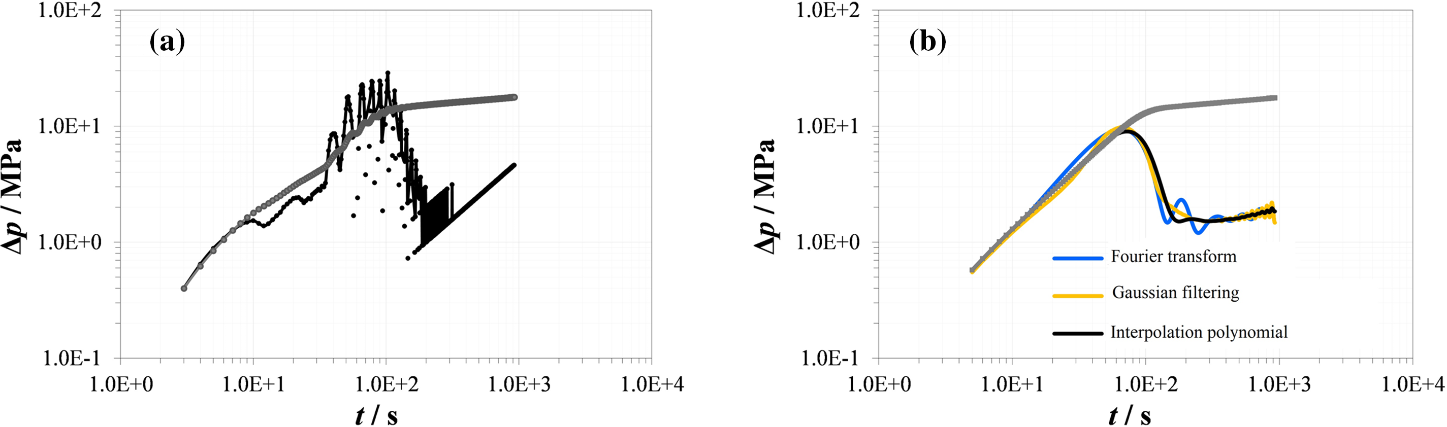
Figure 2: Comparison of typical well testing curves of original data and the data after denoising during the pumping shut-in stage of hydraulic fracturing. (a) Original data, (b) after denoising
2.3 Construction of the Transient Seepage Model Based on Multi-Connected Region Boundary Element Method
As shown in Fig. 3, Ω1 represents the outer region, Ω2 … Ωn + 1 represent SRV (Stimulated Reservoir Volume) regions, Γ1 represents the outer boundary of the outer region, Γ2 … Γn + 1 represents the boundary of the SRV regions. xm represents the width of the SRV region, and ym represents its length. Similarly, xe represents the width of the USRV (Unstimulated Reservoir Volume) region and ye represents its length. The basic assumptions of the model are as follows:
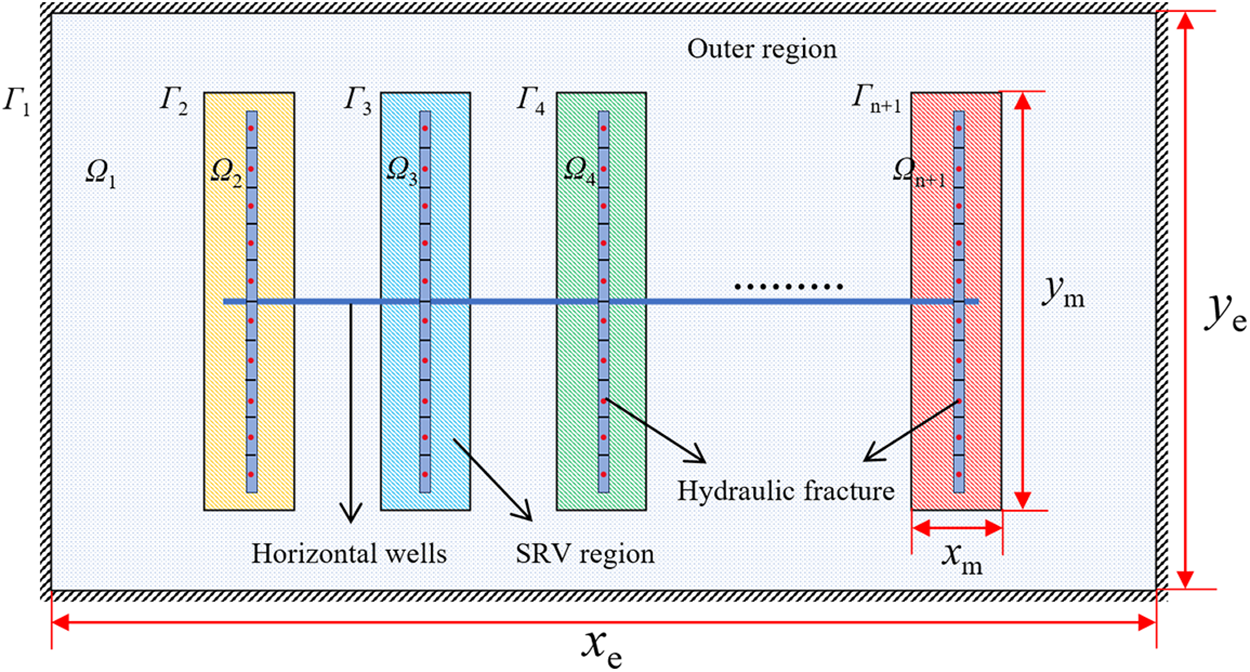
Figure 3: The schematic diagram of the physical model
(1) The shale matrix is a dual-porosity medium model consisting of both pores and natural fractures. (2) Only the leakage of fracturing fluid from hydraulic fractures to natural fractures is considered, ignoring the imbibition of fracturing fluid in shale matrix pores. (3) The closure of fractures during the pumping shut-in stage is considered as the stress sensitivity effect, characterized by the exponential function relationship between fracture permeability and pressure (4) Ignoring migration of proppant particles during the pumping shut-in stage.
By utilizing the method of point source function, incorporating pseudo-pressure, dimensionless variables, and Laplace transformation, we derive the governing equations for both the inner and outer regions, along with the flux equation. The governing equation for fluid flow in the outer region is:
where
The governing equation for fluid flow in the inner region is:
where
The expression for the advection term can be written as:
where λ is the transmissibility coefficient;
The initial conditions are specified as follows:
The outer boundary condition is:
The interface conditions between the internal and external regions are defined as follows:
The Laplace space fundamental solution for the implementation of the boundary element method is presented as:
where P and Q denote arbitrary points either within the domain or on the boundary; K0() is second kind of modified Bessel function.
The outer boundary Γ1 can be divided into N1 linear segments, whereas the inner boundaries Γ2 … Γn + 1 can be partitioned into N2 … Nn + 1 segments. The numbering scheme for boundary discretization and the integration order are illustrated as shown in Fig. 4.
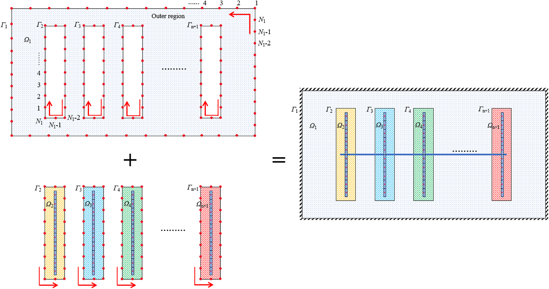
Figure 4: Schematic diagram of boundary discretization and integration sequence
By using the boundary element method, the boundary integral equation for the outer region boundary element in Laplace space can be expressed as:
The boundary integral equation for the inner region boundary element is given by:
where the Qk represents k-th point; P’ denotes any point on the boundary node; θ is a constant coefficient associated with the geometric shape at the point Q.
where α represents the angle between the boundary tangent at point Q.
The boundary integral equation for the discretized center points of fracture segments within the internal domain can be written as:
where
Considering the stress sensitivity of the hydraulic fracture, we utilize an exponential form to depict the permeability variation. Then, the governing equation of hydraulic fracture can be obtained:
where γ is the permeability modulus of the fracture, τ is the ratio of the outer region to the hydraulic fracture conductivity coefficient, pFDi is the dimensionless initial hydraulic fracture pressure, pFD is the dimensionless hydraulic fracture pressure.
Through the substitution of the Pedrosa variables and perturbation transformations, the Eq. (17) can be written as:
The equation satisfied by ψD is:
After discretizing the fracture model in the Laplace space:
where LDi,n is the dimensionless distance from the horizontal well to the n-th segment of the hydraulic fracture in the i-th internal region, RFD is the dimensionless conductivity of the hydraulic fractures.
The production condition for the horizontal well is expressed as:
By solving
And bottom-hole pressure can be obtained with wellbore storage coefficient and skin factor.
where CD is the dimensionless well storage coefficient, Sk is the skin factor.
Ultimately, employing the Stehfest numerical inversion algorithm [32], we derive the real-space ψwD. Then, based on Eq. (19), we compute the bottom-hole pseudo-pressure pwD.
2.4 Model Validation and Sensitivity Analysis
The semi-analytical model is validated by Saphir well-testing software. The simplified model is shown in Fig. 5, the reservoir is a closed system, and each SRV region is considered to be independent of one another. The basic parameters are shown in Table 3.
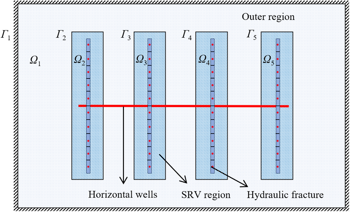
Figure 5: Schematic diagram of simplified model
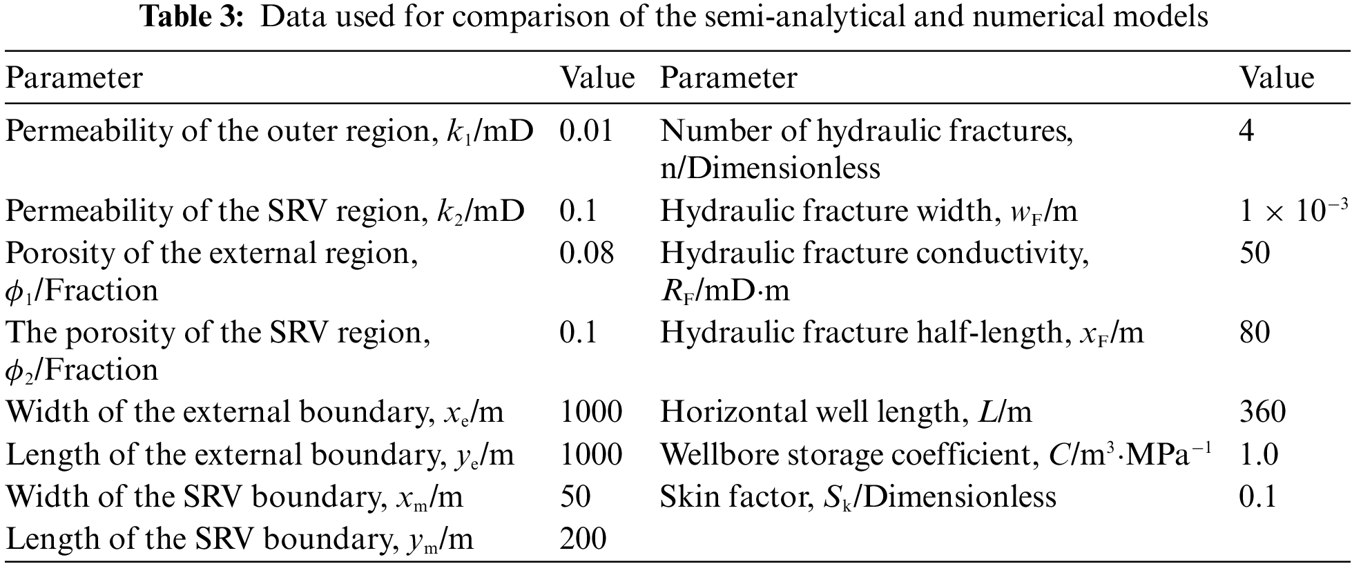
Subsequently, we input the parameters shown in Table 3 into both models for computation and comparison of the results (As shown in Fig. 6). The results indicate that the Saphir numerical model and our semi-analytical model have a high degree of match, demonstrating the reliability of our model. Additionally, during the computation process, we found that the semi-analytical model has a significantly faster computation speed compared to the numerical model, which also highlights the advantage of our model. We also observed a slight difference in the calculation results of the two models at 5000 h. This discrepancy is due to the Saphir numerical model not refining the mesh at the boundary of the SRV region during the mesh discretization process, leading to errors in the Saphir model’s calculations for this area.
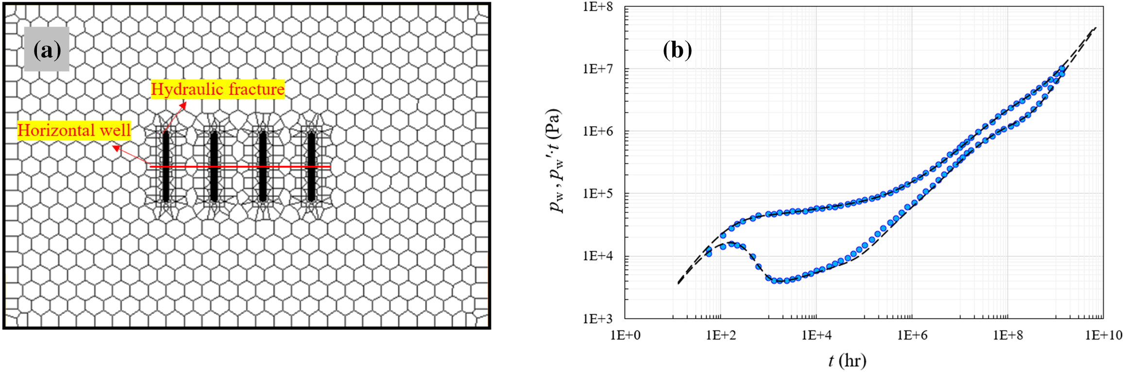
Figure 6: Schematic diagram of model validation. (a) Grid system of Saphir model. (b) Fit results
2.4.2 Effect of SRV Region Size
In this section, the dimensionless pressure response for a fractured horizontal well in a shale gas reservoir is calculated and type curves are plotted based on the basic data given in Table 4. As shown in Fig. 7, five flow regimes are identified as follows:
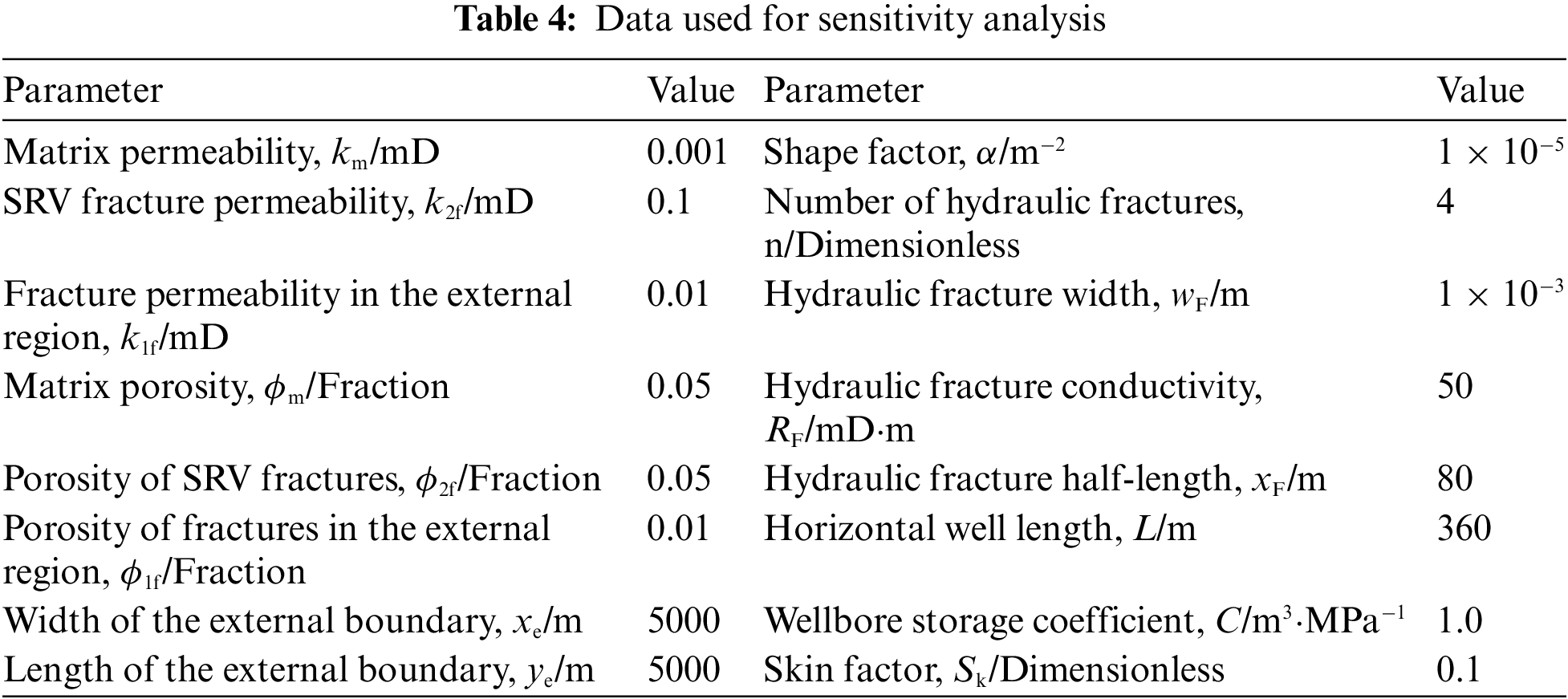
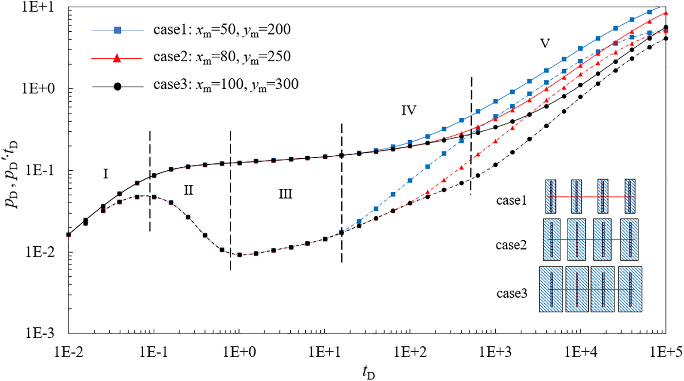
Figure 7: Effect of SRV region size on type curves (Solid Line: Pressure Differential, Dashed Line: Derivative)
Stage I is the wellbore storage stage. The pressure and its derivative curve are straight lines with a unit slope. Stage II is the transient flow stage. The pressure derivative curve has the obvious form of rising and falling in this stage. Stage III is the bilinear flow stage with the slope of the pD′ – tD curve in the typical log-log plot equals 1/4. Stage IV is the linear flow stage. The curve of the dimensionless pressure derivate vs. dimensionless time in the typical curve has a 1/2 slope. Stage V is the transition stage between the inner region and the outer region, where the slope of the pressure derivative curve increases with the difference in permeability between the inner region and the outer region.
Fig. 7 shows the effects of the SRV region size on the type curve. From Fig. 7, it can be observed that the effect of the SRV region size is mainly on the linear flow stage (Stage IV) and the transition stage between the inner and outer regions (Stage V). As the SRV area increases, the transition stage between the inner and outer regions (Stage V) occurs later, extending the linear flow time in the SRV area.
2.4.3 Effect of Permeability of the SRV Region
Fig. 8 shows the effect of differences in properties within the SRV area on the type curve. Due to varying permeabilities across different SRV regions, significant differences exist in the type curves. As shown in Fig. 8, the effect of the SRV region permeability is mainly on the transition stage (Stage II), bilinear flow (Stage III), and linear flow stage (Stage IV). With increasing permeability, the transient flow stage and bilinear flow stage appear earlier.
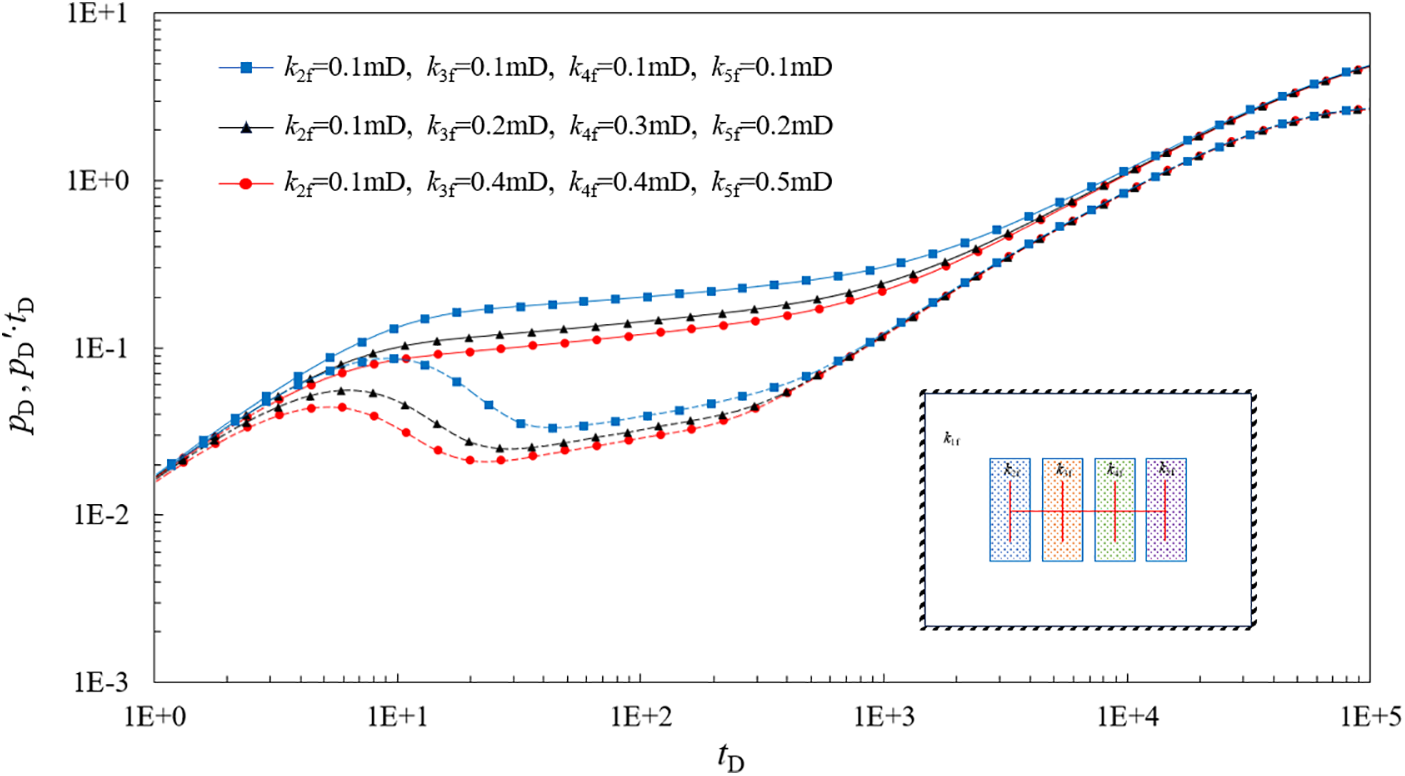
Figure 8: Effect of different permeability in SRV region on typical well test curves (Solid Line: Pressure Differential, Dashed Line: Derivative)
2.4.4 Effect of the Fracture Conductivity
The effect of hydraulic fracture conductivity on the type curve is illustrated in Fig. 9. The conductivity of hydraulic fractures primarily influences the transition stage (Stage II), bilinear flow (Stage III), and linear flow stage (Stage IV). The larger the value of the hydraulic fracture conductivity becomes, the lower the type curves of the transition stage are. Moreover, as the value of the hydraulic fracture conductivity increases, the bilinear flow stage becomes shorter while the linear flow stage becomes longer.
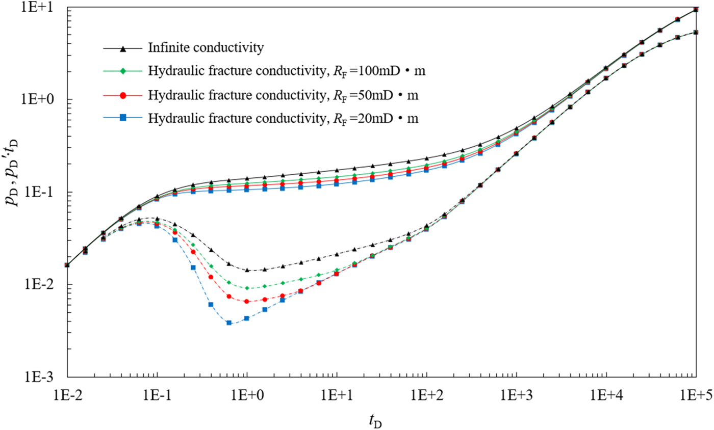
Figure 9: Effect of different fracture conductivity on typical well test curves (Solid Line: Pressure Differential, Dashed Line: Derivative)
2.4.5 Effect of the Hydraulic Fracture Length
Fig. 10 shows the effect of the length of hydraulic fractures on the type curve. As the length of hydraulic fractures increases, the type curve is higher. The pressure derivative curve declines more rapidly during the transition flow stage (Stage II). The impact of varying hydraulic fracture length on the well test curve persists until the transition stage between the inner and outer zones (Stage V). Moreover, with an increase in the length of hydraulic fractures, the distance from the hydraulic fractures to the boundary of the SRV area decreases, which results in a shorter transition stage. Conversely, when there are short hydraulic fractures within the SRV area, a trend toward radial flow may appear. It indicates that the model is sensitive to hydraulic fracture length, making it reliable for inversion of the fracture parameters.
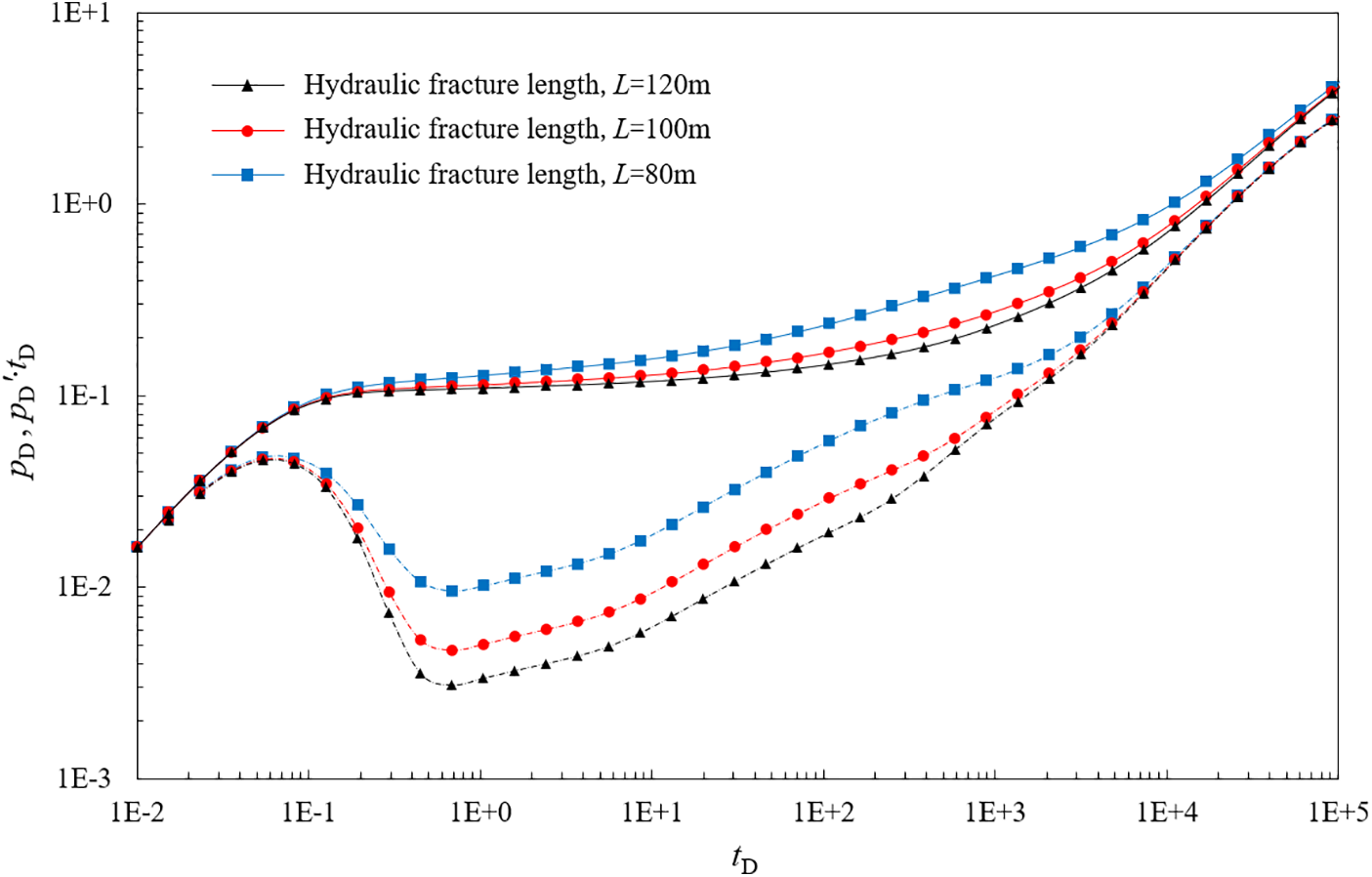
Figure 10: Effect of hydraulic fractures length on typical well test curves (Solid Line: Pressure Differential, Dashed Line: Derivative)
2.4.6 Effect of Hydraulic Fracture Numbers
Fig. 11 shows the effect of the hydraulic fracture numbers on the type curve. The larger the number of hydraulic fractures is, the longer the transition flow stage (Stage II) is. Moreover, the pressure curve and the pressure derivative curve are lower. It indicates that the model is sensitive to hydraulic fracture numbers, making it reliable for inversion of the fracture parameters.
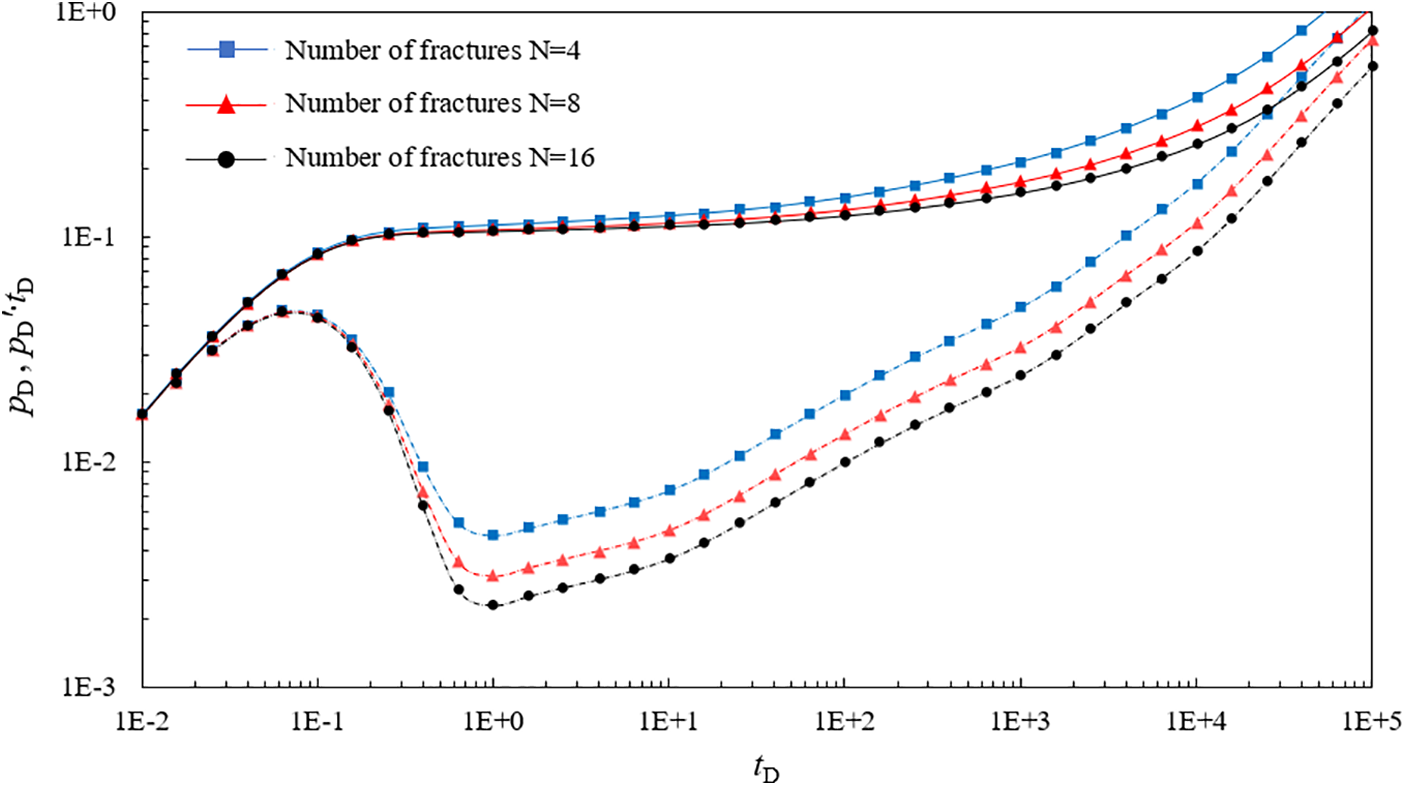
Figure 11: Effect of different hydraulic numbers on typical well test curves (Solid Line: Pressure Differential, Dashed Line: Derivative)
2.5 Workflow of Hydraulic Fracture Parameters Inversion Based on Pumping Shut-in Pressure-Drop Data
This paper establishes a workflow for hydraulic fracture parameter inversion based on pumping shut-in pressure drop data. First, construction data is collected to convert pumping pressure to bottomhole pressure. And Gaussian filtering is then used to denoise the data, obtaining the data for well test analysis. And then, a transient flow model for shale gas wells based on the boundary element method is established. With the model parameters are adjusted to fit the pressure data as closely as possible, the single stage fracture parameters can be obtained. The work flow is shown in the Fig. 12.
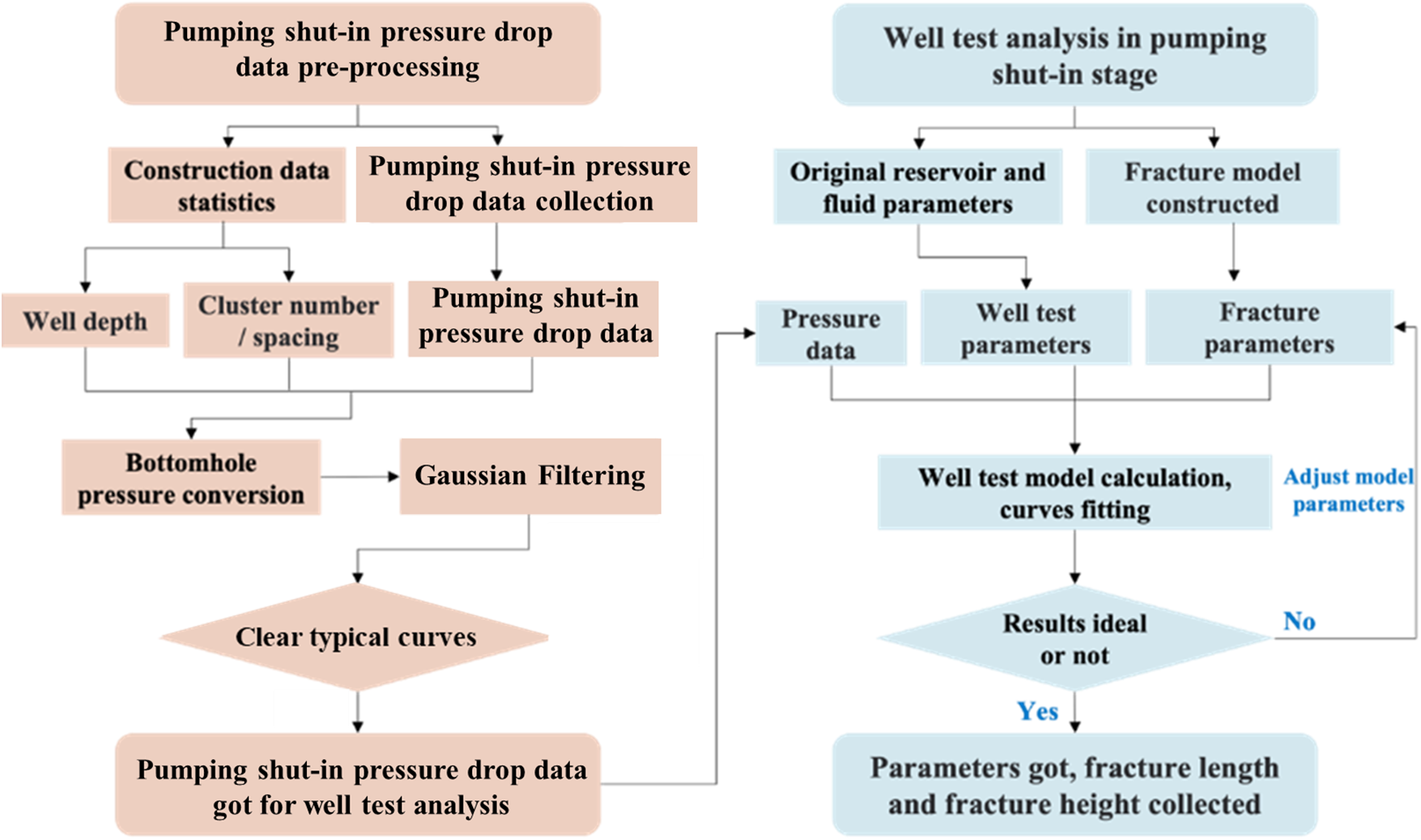
Figure 12: Workflow of fracture parameters inversion based on pressure-drop data of pumping shut-in stage
The methodology proposed in this paper was put into practice with actual wells in the Changning shale gas well area, yielding parameters for individual fracture segments in shale reservoirs, including fracture half-length xF, total length of single-stage fractures LtF, average height of single-stage fractures hF, and fracture surface area StF.
Initially, we utilized actual gas production profile test data from the Changning HX-9 well to validate the rationality of the parameter interpretation results in this study. Fig. 13 illustrates the porosity, relative total organic carbon content (TOC), and gas production capability ratio of different fracturing stages at various stratigraphic positions in the HX-9 well.
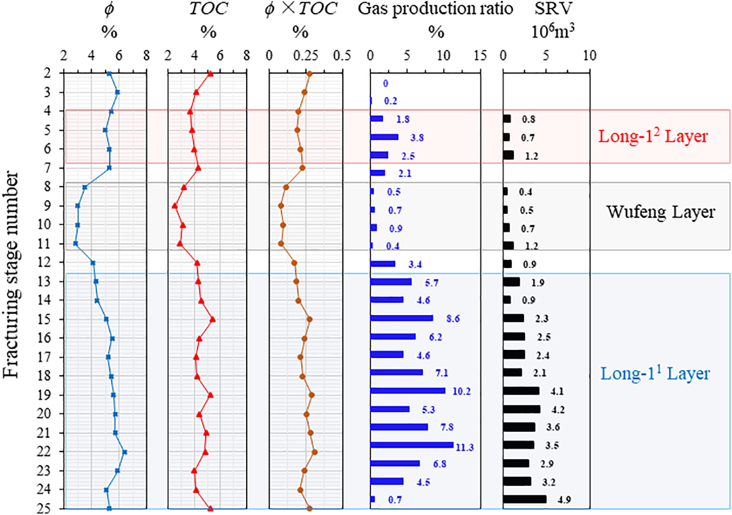
Figure 13: Reservoir physical property, gas production profile test results, and single segment SRV of well HX-9
From Fig. 13, it is evident that the proportion of gas production from each fracturing stage in the well is significantly correlated with its formation position. This correlation arises from differences in reservoir gas content, reservoir properties, and hydraulic fracturing effects across different formations. Therefore, to comprehensively analyze the influencing factors on shale gas well productivity, it is necessary to consider both engineering parameters and reservoir property parameters. The methodology proposed in this study serves as a systematic approach to address this requisite. The inversion results of single-stage fracture parameters in the HX-9 well are shown in Figs. 14 and 15.
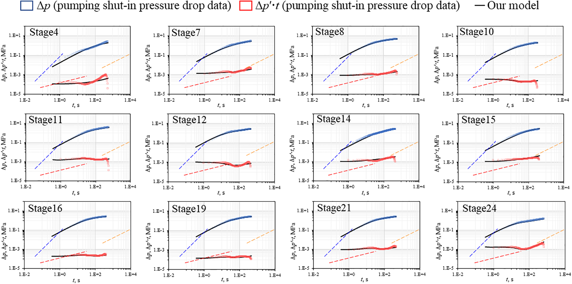
Figure 14: The curve fitting results of well HX-9
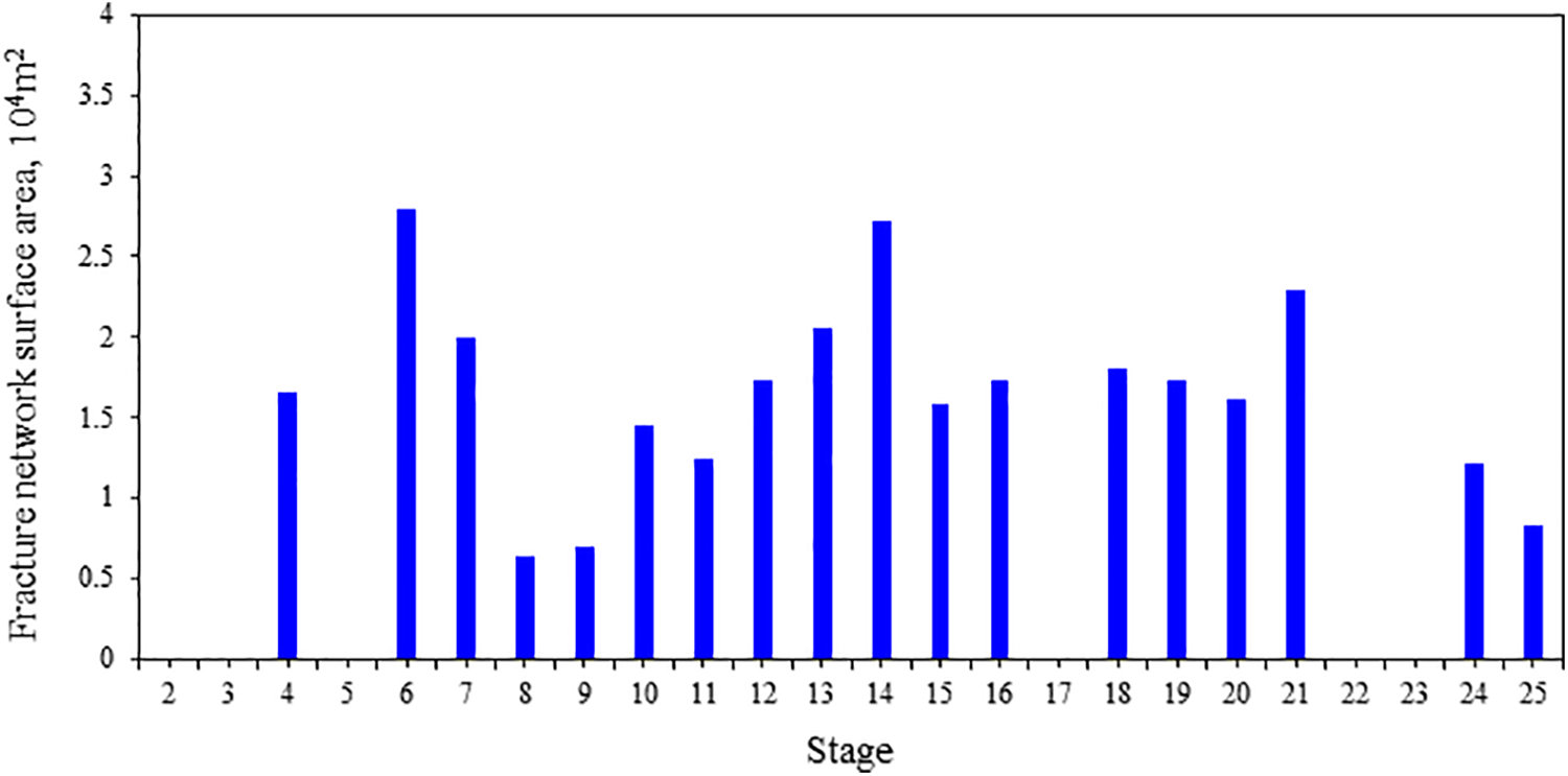
Figure 15: Single-segment total fracture surface area of well HX-9 (Where the missing data is attributed to inadequate pumping shut-in time, rendering the method inapplicable)
Integrating the results of fracture surface area inversion, gas production profile test data, porosity, and TOC content data from well HX-9, we analyzed the factors contributing to variations in gas well productivity.
Fig. 16a shows the correlation curve between the product of TOC content rTOC, porosity ϕ and the gas production ratio Rgp of the HX-9 well. It can be observed that the Rgp of the Long-11 layer and Wufeng-Long-12 fracturing stages exhibit a relatively independent correlation with rTOC × ϕ, indicating a lower correlation. By constructing a combined parameter of porosity, TOC, and fracture surface area StF as rTOC × ϕ × StF, and comparing it with the gas well production ratio Rgp (as shown in Fig. 16b), it is evident that the combined parameter rTOC × ϕ × StF exhibits a significantly stronger correlation with Rgp. This reflects the accuracy of the parameter interpretation method proposed in this study, while also revealing that analyzing differences in gas production capability between well segments requires a comprehensive consideration of reservoir properties and single-segment fracture parameters.
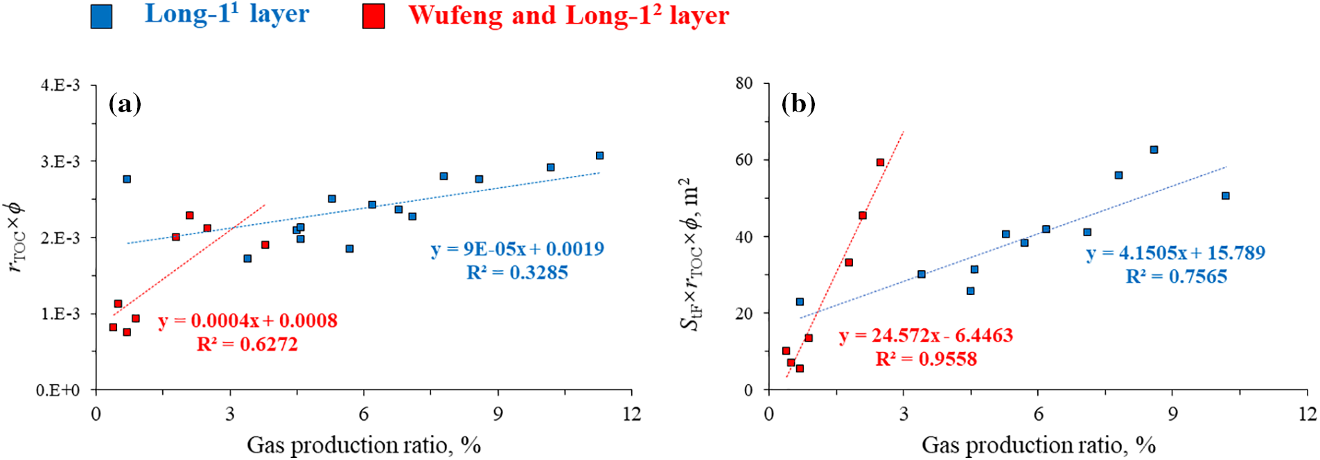
Figure 16: Correlation of single segment gas production ratio in HX-9 well. (a) rTOC × ϕ and gas production ratio, (b) StF × rTOC × ϕ and gas production ratio
Furthermore, utilizing the hydraulic fracture parameters inversion, we evaluated the relationship between fracturing effectiveness and engineering parameters, as well as reservoir property parameters.
Fig. 17 demonstrates a negative linear correlation between the cluster number and single-stage hydraulic fracture half-length, indicating that the fewer the cluster number is, the longer the single-stage fracture half-length is. Additionally, the correlation between the average fracture height and the single-segment cluster number shows a similar trend. It indicates that with fewer cluster numbers, the net fracture pressure decreases, making it more challenging for the fracture height to expand.
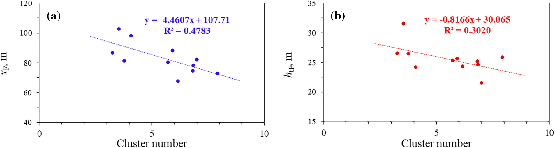
Figure 17: Correlation between fracture half-length, average fracture height and cluster number. (a) Cluster number and xF, (b) Cluster number and htF
Fig. 18 illustrates the correlation curve between the total hydraulic fracture length of the single segment with cluster number and spacing. Horizontal wells with a higher number of clusters and lower spacing tend to exhibit longer total fracture lengths of a single stage. Additionally, there is a notable negative linear correlation between the volume of fluid injection per stage per meter (Hf) and the total fracture length of a single segment, and a positive correlation with the fracture half-length of a single segment (as shown in Fig. 19). It indicates that the larger the volume of fluid injection per stage per meter is, the longer the fracture half-length of the single segment is. Conversely, a larger volume of fluid injected per stage per meter corresponds to a shorter total fracture length of a single segment. It indicates that merely increasing pump injection rates will not significantly enhance hydraulic fracture dimensions; instead, fracturing optimization requires the joint adjustment of cluster number and spacing.
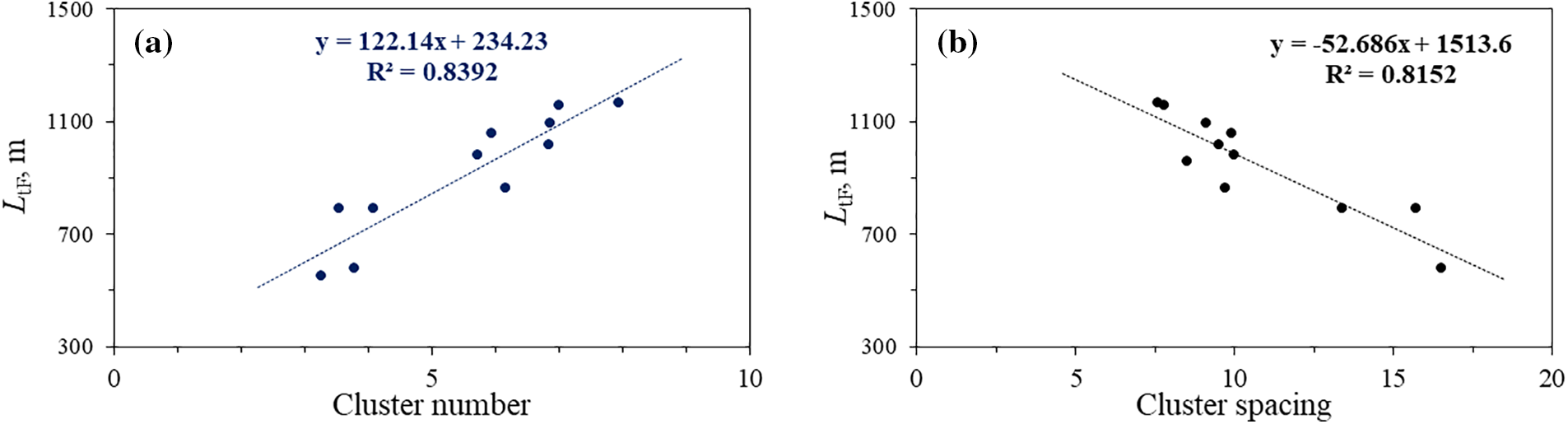
Figure 18: Correlation between cluster number and cluster spacing and total fracture length of single segment. (a) LtF and cluster number, (b) LtF and cluster spacing
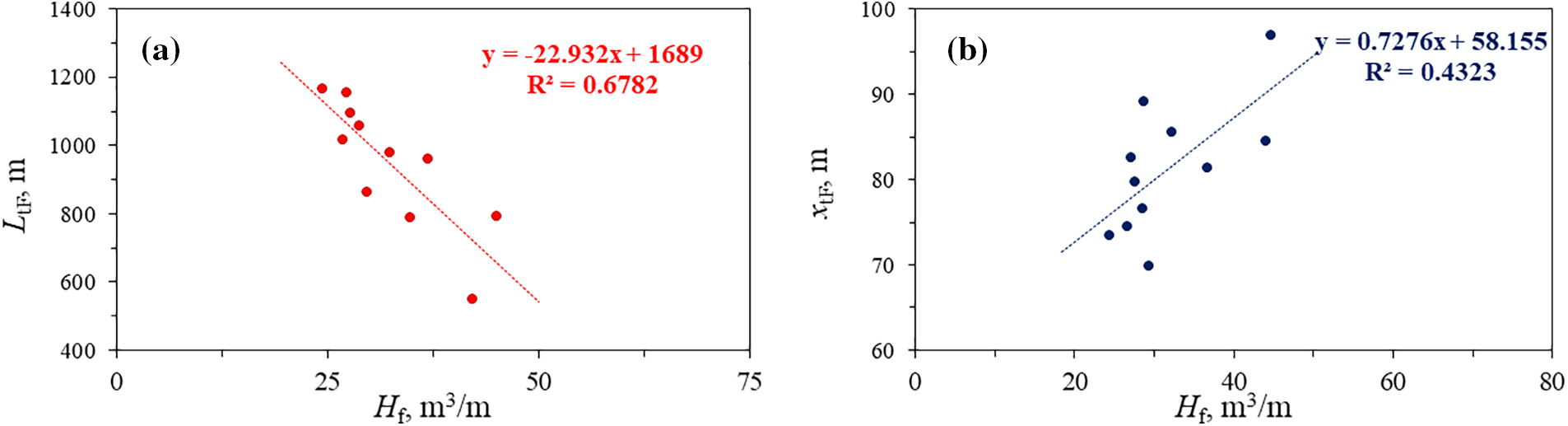
Figure 19: Correlation between total fracture length of single segment, fracture half-length and the volume of fluid injection of per stage per meter. (a) Hf and LtF, (b) Hf and xF
Fig. 20 shows a negative correlation between the horizontal stress difference Δσ and the total hydraulic fracture length of a single stage. As the horizontal stress difference increases, the extension of fractures becomes more challenging, leading to a relatively smaller total fracture length of a single segment. Despite the horizontal stress difference being similar between different stages of the same well, it still exhibits a negative linear correlation with the total fracture length of a single segment. This highlights the importance of the horizontal stress difference in controlling the total fracture length of a single segment.
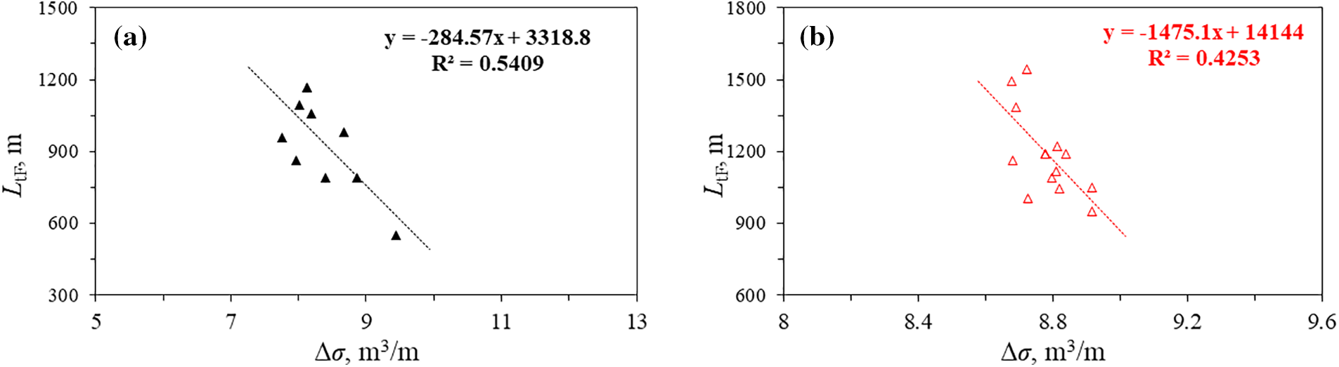
Figure 20: Correlation between horizontal stress difference and total fracture length of single segment. (a) the correlation between the Δσ among different wells and the average fracture length LaF of the entire well. (b) The correlation between the Δσ among different stage within the same well and the LtF
In addition to the variation in in-situ horizontal stress difference, natural fracture density is also a crucial factor influencing the hydraulic fracturing effectiveness of shale gas wells. By utilizing dimensionless natural fracture density logging interpretation data from the Changning HX platform area (as shown in Fig. 21), the impact of natural fracture density on hydraulic fracture parameters in the Changning shale gas well area was analyzed.
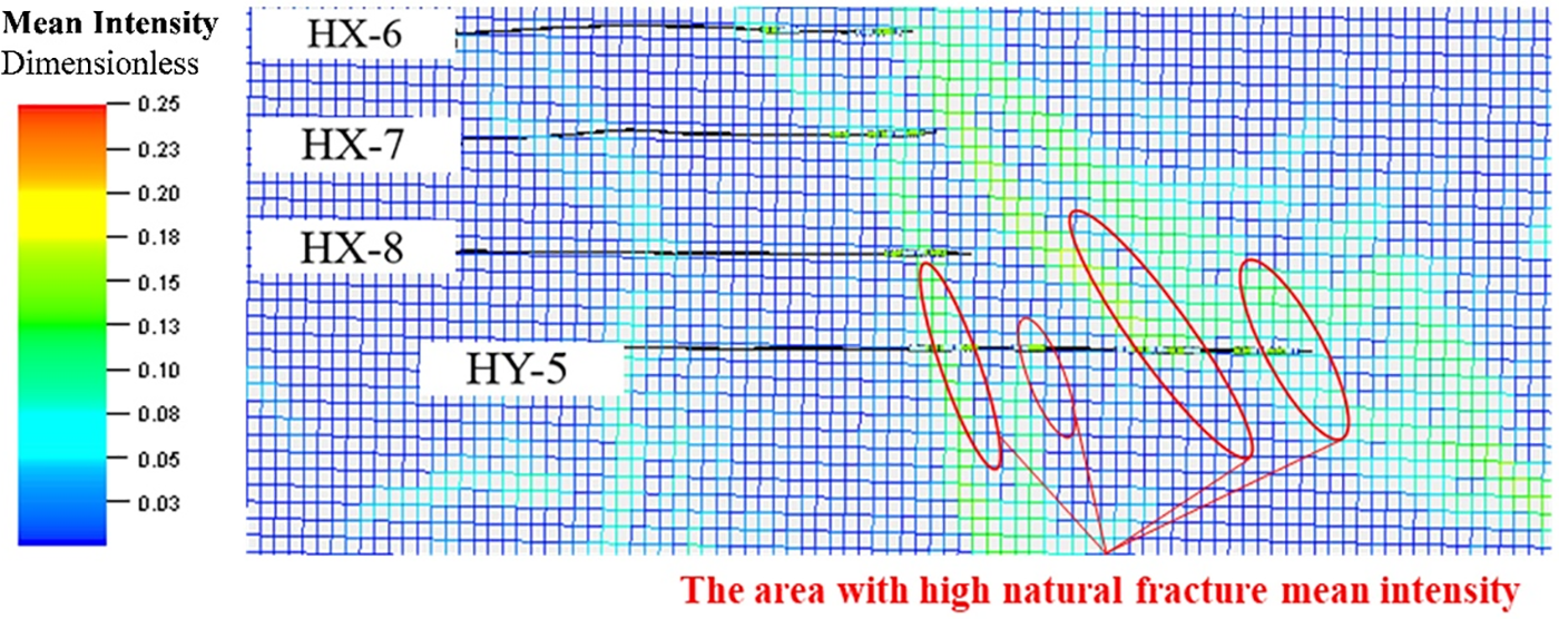
Figure 21: Natural fracture intensity distribution
Fig. 22 shows the correlation between the intensity of natural fracture If and the total fracture length of a single segment. Fig. 22a shows the correlation curves between the single-stage total fracture length and the natural fracture intensity for each of the three wells. With an increase in the If, the total fracture length of a single stage shows a notable increase. However, beyond a threshold value of approximately 0.075, the total fracture length of a single stage begins to decrease with further increases in natural fracture mean intensity. This trend is consistent with the correlation between natural fracture mean intensity and total fracture length of a single stage (Fig. 22b). Thus, inversion results based on single-stage fracture parameters can provide effective evidence for analyzing the impact of natural fracture mean intensity on fracture parameters.
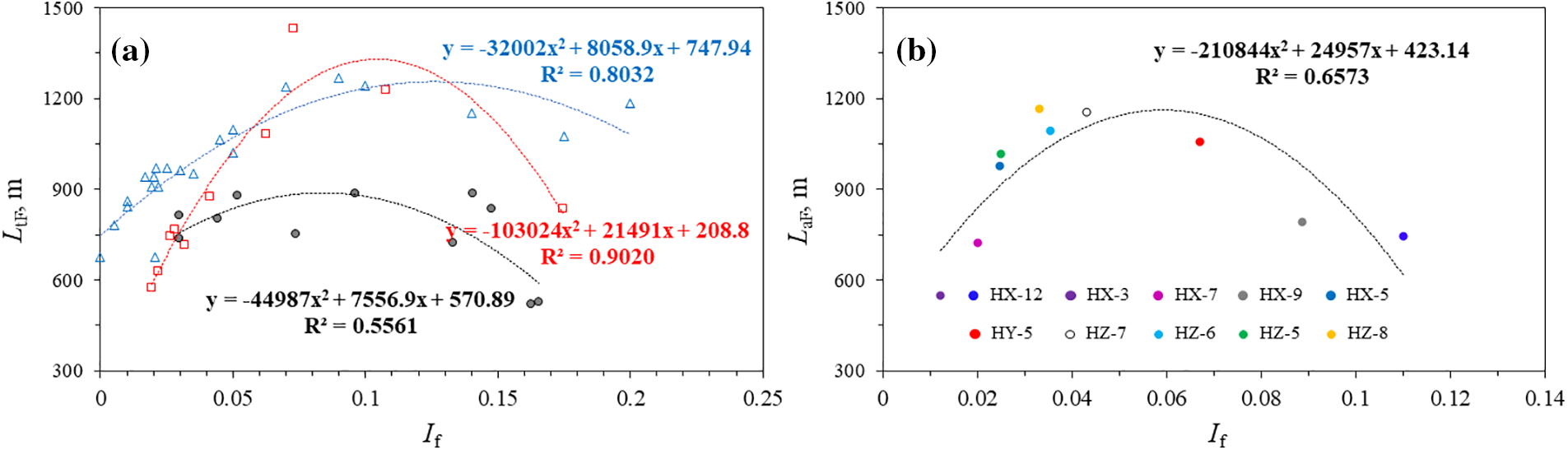
Figure 22: Correlation between the natural fractures mean intensity and total fracture length of single stage. (a) If and LtF (different colors represent different wells), (b) If and LaF
In this paper, the characteristics of the existing fracture parameters inversion and evaluation methods are systematically sorted out. A work flow of ‘pre-processing of pumping shut-in stage data–establishment of semi-analytical model–well testing interpretation’ of hydraulic fracture parameters inversion is established. The method is applied to the Changning shale gas well area. The main conclusions are as follows:
(1) The inversion of hydraulic fracture parameters based on pumping shut-in data does not require long-time well shut-in pressure testing. Simultaneously, it enables the inversion of fracture parameters of single segment.
(2) The length of hydraulic fracture and the number of hydraulic fracture exhibit high sensitivity to type curve, which indicates that our model is suitable for interpreting fracture parameters. Practical application shows that a shut-in time of around 15 min is needed for effective pressure decline analysis; otherwise, typical curves may not be plotted.
(3) The correlation between gas production profile test data from typical wells and hydraulic fracture parameters of single stage indicates that employing comprehensive parameters of reservoir properties and hydraulic fracture parameters provides a more accurate explanation of the difference in gas productivity across different fracturing segments.
(4) The accuracy of fracture parameter inversion results based on pumping shut-in pressure-drop data is high, offering significant advantages in evaluating fracturing effectiveness using single stage fracture parameters.
Although the current work has achieved satisfactory results, there are issues that need to be addressed in future research. For example, developing a flow model that considers gas-water two-phase unsteady flow and constructing a well test interpretation model that couples wellbore flow with reservoir flow. This would help solve the problem of fracture parameter inversion when there are depth differences between different fracturing stages in horizontal wells.
Acknowledgement: We have referenced and cited many scholars and would first like to thank these scholars for their efforts and contributions in this regard. Secondly, we would like to thank the Complex Gas Reservoir Theory and Application Team of Southwest Petroleum University for their help in this research, including model validation, and example applications.
Funding Statement: This research was funded by the Science and Technology Cooperation Project of the CNPC-SWPU Innovation Alliance, grant numbers “2020CX020202, 2020CX030202 and 2020CX010403”.
Author Contributions: Shangjun Gao: Conceptualization; methodology; validation; formal analysis; writing—original draft preparation; project administration. Yang Yang: Conceptualization; validation; investigation. Man Chen: Software; validation; resources; data curation. Jian Zheng: Software; validation; resources. Luqi Qin: Writing—review and editing. Jianying Yang: Visualization; supervision. Xiangyu Liu: Writing—review and editing. All authors reviewed the results and approved the final version of the manuscript.
Availability of Data and Materials: The data that support the findings of this study are available from the corresponding author, Luqi Qin, upon reasonable request.
Ethics Approval: Not applicable.
Conflicts of Interest: The authors declare that they have no conflicts of interest to report regarding the present study.
References
1. Y. M. Sun, S. D. Li, C. Lu, S. M. Liu, W. C. Chen and X. Li, “The characteristics and its implications of hydraulic fracturing in hydrate-bearing clayey silt,” J. Nat. Gas Sci. Eng., vol. 95, no. 2, pp. 104–114, Nov. 2021. doi: 10.1016/j.jngse.2021.104189. [Google Scholar] [CrossRef]
2. M. Cai, W. Wang, X. J. Wang, L. Zhao, and H. T. Zhang, “Characteristics of hydraulic fracture penetration behavior in tight oil with multi-layer reservoirs,” Energy Rep., vol. 10, no. 2, pp. 2090–2102, Nov. 2023. doi: 10.1016/j.egyr.2023.08.089. [Google Scholar] [CrossRef]
3. C. Z. Zang et al., “An analysis of the uniformity of multi-fracture initiation based on downhole video imaging technology: A case study of Mahu tight conglomerate in Junggar Basin, NW China,” Pet. Explor. Dev., vol. 49, no. 2, pp. 394–402, Apr. 2022. doi: 10.1016/S1876-3804(22)60038-7. [Google Scholar] [CrossRef]
4. B. Hou, M. Chen, Z. M. Li, Y. H. Wang, and C. Diao, “Propagation area evaluation of hydraulic fracture networks in shale gas reservoirs,” Pet. Explor. Dev., vol. 41, no. 6, pp. 833–838, Dec. 2014. doi: 10.1016/S1876-3804(14)60101-4. [Google Scholar] [CrossRef]
5. S. J. Wu et al., “Distribute fiber optic micro-vibration monitoring in offset-well and microseismic source location imaging during horizontal well fracturing in shale gas reservoir,” J. Chin. J. Geophys., vol. 65, no. 7, pp. 2756–2765, Jul. 2022. doi: 10.6038/cjg2022P0658. [Google Scholar] [CrossRef]
6. D. W. H. Su, P. Zhang, H. Dougherty, M. Van Dyke, and R. Kimutis, “Longwall mining, shale gas production, and underground miner safety and health,” Int. J. Min. Sc. Techno., vol. 31, no. 3, pp. 523–529, Jan. 2021. doi: 10.1016/j.ijmst.2020.12.013. [Google Scholar] [CrossRef]
7. M. H. Wei et al., “A three-axis antenna to measure near-field low-frequency electromagnetic radiation generated from rock fracture,” Measurement, vol. 173, no. 3, pp. 1–13, Mar. 2021. doi: 10.1016/j.measurement.2020.108563. [Google Scholar] [CrossRef]
8. J. J. Liu, L. W. Jiang, T. J. Liu, and D. Y. Yang, “Modeling tracer flowback behavior for a fractured vertical well in a tight formation by coupling fluid flow and geomechanical dynamics,” J. Nat. Gas Sci. Eng., vol. 84, Dec. 2020, Art. no. 103656. doi: 10.1016/j.jngse.2020.103656. [Google Scholar] [CrossRef]
9. M. Chen et al., “Evolution mechanism of optical fiber strain induced by multi-fracture growth during fracturing in horizontal wells,” Pet. Explor. Dev., vol. 49, no. 1, pp. 211–222, Nov. 2022. doi: 10.1016/S1876-3804(22)60017-X. [Google Scholar] [CrossRef]
10. H. T. Li et al., “DTS based hydraulic fracture identification and production profile interpretation method for horizontal shale gas wells,” Nat. Gas. Ind., vol. 8, no. 5, pp. 494–504, Oct. 2021. doi: 10.1016/j.ngib.2021.05.001. [Google Scholar] [CrossRef]
11. E. Siebrits and A. P. Peirce, “An efficient multi-layer planar 3D fracture growth algorithm using a fixed mesh approach,” Int. J. Numer. Methods Eng., vol. 53, no. 3, pp. 691–717, Nov. 2001. doi: 10.1002/nme.308. [Google Scholar] [CrossRef]
12. X. Weng, O. Kresse, and C. Cohen, “Modeling of hydraulic-fracture-network propagation in a naturally fractured formation,” SPE Prod. Oper., vol. 26, no. 4, pp. 368–380, Nov. 2011. doi: 10.1007/s11831-021-09653-z. [Google Scholar] [CrossRef]
13. H. Y. Tang, H. P. Liang, L. H. Zhang, and H. Y. Li, “Fully 3D simulation of hydraulic fracture propagation in naturally fractured reservoir using displacement discontinuity method,” SPE J., vol. 27, no. 3, pp. 1648–1670, Jun. 2022. doi: 10.2118/209219-PA. [Google Scholar] [CrossRef]
14. B. Chen and B. R. Barboza, “A review of hydraulic fracturing simulation,” Arch. Comput., vol. 9, no. 4, pp. 1–58, Oct. 2021. doi: 10.1007/s11831-021-09653-z. [Google Scholar] [CrossRef]
15. P. Yang et al., “Numerical simulation of integrated three-dimensional hydraulic fracture propagation and proppant transport in multi-well pad fracturing,” Comput. Geotech., vol. 167, Mar. 2024, Art. no. 106075. doi: 10.1016/j.compgeo.2024.106075. [Google Scholar] [CrossRef]
16. X. Q. Wang, D. T. Lu, and P. C. Li, “A novel hybrid model for hydraulic fracture simulation based on peri-dynamic theory and extend finite element method,” Theor. Appl. Fract. Mech., vol. 123, Feb. 2023, Art. no. 103731. doi: 10.1016/j.tafmec.2022.103731. [Google Scholar] [CrossRef]
17. M. Y. Soliman, C. Miranda, H. Wang, and K. Thornton, “Investigation of effect of fracturing fluid on after-closure analysis in gas reservoir,” SPE Prod. Oper., vol. 26, no. 2, pp. 185–194, Mar. 2011. doi: 10.2118/128016-PA. [Google Scholar] [CrossRef]
18. S. Hossain, H. Dehghanpour, O. Ezulike, B. Dotson, and S. Motealleh, “Port-Opening falloff test: A complementary test to diagnostic fracture injection test,” SPE J., vol. 27, no. 6, pp. 3363–3383, Dec. 2022. doi: 10.2118/209601-PA. [Google Scholar] [CrossRef]
19. G. Liu and C. Ehlig-Economides, “Comprehensive before-closure model and analysis for fracture calibration injection falloff test,” J. Petrol. Sci. Eng., vol. 172, no. 12, pp. 911–933, Jan. 2019. doi: 10.1016/j.petrol.2018.08.082. [Google Scholar] [CrossRef]
20. R. Y. Yang et al., “A semi-analytical approach to model two-phase flowback of shale-gas wells with complex-fracture-network geometries,” SPE J., vol. 22, no. 6, pp. 1808–1833, Aug. 2017. doi: 10.2118/181766-PA. [Google Scholar] [CrossRef]
21. V. Sahai, G. Jackson, H. Lawal, N. Abolo, and C. Flores, “A quantitative approach to analyze fracture-area loss in shale gas wells during field development and resimulation,” SPE Reserv. Eval. Eng., vol. 18, no. 3, pp. 346–355, Aug. 2015. doi: 10.2118/169406-PA. [Google Scholar] [CrossRef]
22. Y. C. Cui, R. Z. Jiang, Y. H. Gao, and J. Q. Lin, “Semi-analytical modeling of rate transient for a multi-wing fractured vertical well with partially propped fractures considering different stress-sensitive systems,” J. Petrol. Sci. Eng., vol. 208, Jan. 2022, Art. no. 109548. doi: 10.1016/j.petrol.2021.109548. [Google Scholar] [CrossRef]
23. P. Chen, S. Jiang, Y. Chen, and K. Zhang, “Pressure response and production performance of volumetric fracturing horizontal well in shale gas reservoir based on boundary element method,” Eng. Anal., vol. 87, no. 3, pp. 66–77, Feb. 2018. doi: 10.1016/j.enganabound.2017.11.013. [Google Scholar] [CrossRef]
24. J. Iriarte, J. Merritt, and B. Kreyche, “Using water hammer characteristics as a fracture treatment diagnostic,” presented at SPE Okla. City Oil Gas Sym., Oklahoma City, OK, USA, Mar. 27, 2017. doi: 10.2118/185087-MS. [Google Scholar] [CrossRef]
25. N. Dung, C. David, and D. Tom, “Practical applications of water hammer analysis from hydraulic fracturing treatments,” presented at 2021 SPE Hydr. Frac. Tech. Conf., May 2021. doi: 10.2118/204154-MS. [Google Scholar] [CrossRef]
26. G. Liu, T. Zhou, and F. Li, “Fracture surface area estimation from hydraulic-fracture treatment pressure falloff data,” SPE Drill., vol. 35, no. 3, pp. 438–451, Sep. 2020. doi: 10.2118/199895-PA. [Google Scholar] [CrossRef]
27. D. Tompkins, S. Persac, Halliburton, “Nitrogen fracture-injection/falloff testing and analysis in under-pressured reservoirs,” presented at the 2016 SPE/AAPG/SEG Uncon. Res. Tech. Conf., San Antonio, TX, USA, Aug. 1–3, 2016. doi: 10.15530/URTEC-2016-2461218. [Google Scholar] [CrossRef]
28. J. Z. Zhao, Y. Q. Fu, and Z. H. Wang, “Study on diagnosis model of shale gas fracture network fracturing operation pressure curves,” Nat. Gas Indus., vol. 42, no. 2, pp. 11–19, Feb. 2022. doi: 10.3787/j.issn.1000-0976.2022.02.002. [Google Scholar] [CrossRef]
29. D. Lee, S. R. Shin, E. -M. Yeo, and W. Chung, “Denoising sparker seismic data with deep BiLSTM in fractional Fourier transform,” Comput. Geosci., vol. 184, no. 3, pp. 1–9, May 2024. doi: 10.1016/j.cageo.2024.105519. [Google Scholar] [CrossRef]
30. M. Mafi, H. Martin, and M. Cabrerizo, “A comprehensive survey on impulse and Gaussian denoising filters for digital images,” Signal Process., vol. 157, no. 3, pp. 236–260, Apr. 2019. doi: 10.1016/j.sigpro.2018.12.006. [Google Scholar] [CrossRef]
31. T. Zhan and W. Zhao, “Fitting algorithm of parameterized continued fractions with keeping endpoints and its application,” Appl. Mech. Mater., vol. 190, pp. 343–346, Jul. 2012. doi: 10.4028/www.scientific.net/AMM.190-191.343. [Google Scholar] [CrossRef]
32. S. Harald, “Algorithm 368: Numerical inversion of Laplace transforms [D5],” Commun. ACM, vol. 13, no. 1, pp. 47–49, Jan. 1970. doi: 10.1145/361953.361969. [Google Scholar] [CrossRef]
Appendix A
The definitions of dimensionless variables are listed as follows:
Dimensionless distance:
Dimensionless pressure, flow rate, time:
Dimensionless permeability modulus and fracture conductance:
Dimensionless wellbore storage coefficient:
Other parameters definition:
Cite This Article
 Copyright © 2024 The Author(s). Published by Tech Science Press.
This work is licensed under a Creative Commons Attribution 4.0 International License , which permits unrestricted use, distribution, and reproduction in any medium, provided the original work is properly cited.
 Downloads
 Citation Tools