Optimized Operation of Park Integrated Energy System with Source-Load Flexible Response Based on Comprehensive Evaluation Index

Nomenclature

1  Introduction

With environmental pollution and energy scarcity on the rise, there is an urgent need to transform China’s energy system from high-carbon to low-carbon, and to this end, China is actively building a low-carbon, clean, and sustainable energy supply system to promote the realization of the goals of carbon peaking and carbon neutrality [1,2]. Integrated energy system (IES), because of its internal coupling of various energy conversion equipment, can realize the interactive conversion of different types of energy, which is of great significance for vigorously developing low-carbon power and improving the consumption capacity of renewable energy [3,4]. Currently, the primary studies on microgrids and IES include system stochasticity and flexibility [5]. References [6,7] considered the system’s uncertainty and constructed the system’s management operation framework to optimize the system operation through the fuzzy primal-dual method of multipliers and stochastic transmission switching integrated interval robust chance-constrained approach, respectively. Reference [8] proposed an intelligent energy management strategy based on the intelligent probabilistic wavelet fuzzy neural network-deep reinforcement learning algorithm considering renewable energy uncertainties and load power variations, which has high efficiency and speed in dealing with all kinds of uncertainties. This paper focuses on the system’s flexibility by introducing some coupling devices to convert and coordinate the energy sources to meet the load demand and improve the economy and flexibility of the system operation.

CHP units have high energy utilization efficiency, which is crucial for solving the energy crisis [9]. Reference [10] proposed a low-carbon economic dispatch model of IES coupled with two-stage power-to-gas equipment and CHP units, which reduces the CHP’s “heat-to-power” operation constraints and facilitates low-carbon economic operation of the system. Reference [11] constructed a flexible response model of CHP units and thermal energy storage system, which can meet the fluctuation of heat load demand and effectively improve the system’s flexibility. Reference [12] introduced an electric boiler (EB) to realize the coupling with CHP, which realized the internal thermoelectric decoupling of the system and fully utilized the excess electricity to meet the heating demand. Reference [13] introduced the organic Rankine cycle (ORC) in the CHP system to convert excess waste heat into electrical energy, thus improving the flexible response to electrical loads. Although the above references address the issue of source-side flexible response to thermal or electric loads, they do not consider the simultaneous flexible response to thermal and electric loads and do not maximize the role of load-side demand response.

Integrated demand response (IDR) is a modification of traditional demand response (DR) for multiple load systems and plays a vital role in IES optimization operation [14]. Reference [15] considered demand response and energy storage system participation in smart microgrid operation, and two-stage energy management through an intelligent probabilistic wavelet petri neuro-fuzzy inference algorithm, which effectively improved the system’s response speed. Reference [16] proposed a stochastic framework for renewable energy integrated microgrid operation and scheduling, which improved demand-side flexibility by unifying the load distribution through demand response. Reference [17] proposed an energy management scheme based on price-elastic demand response for multi-microgrid systems to obtain dynamic energy pricing and load adjustment demand to improve the economic and environmental efficiency of the system. Reference [18] proposed a stochastic objective optimization method for multi-energy system planning, which exploited the flexibility of load-side resources and effectively ensured the synergistic operation of the system. All of the above references have introduced demand response on the load side, but almost few consider flexible response on both the source and load side simultaneously. Therefore, in this paper, while IDR is considered on the load side, the ORC is introduced on the source side to couple with the electric boiler, gas turbine, and waste heat boiler to construct a thermoelectric flexible response CHP unit model, which realizes the thermoelectric flexible response, and thus constructs the source-load flexible response model, which further improves the flexibility of the system.

Reference [19] proposed a novel multi-vector energy system based on electricity, heating, and water generation sources and optimized the economics of the system operation by using a price-based demand response scheme to reduce the final cost throughout the study period. Reference [20] proposed a two-stage optimal scheduling strategy for hybrid energy systems to optimize the economics of the system with the objective of minimizing the system operating cost and maximizing the profit from energy storage, respectively. Reference [21] proposed a day-ahead intra-day optimal dispatch strategy for renewable energy generation and power fluctuation uncertainty, which took system’s operating cost as the optimization objective, and performed a two-stage system optimization to improve the system economics. The above studies were mainly conducted regarding system economics and did not simultaneously consider the influence of the system’s economic, energy efficiency and environmental indicators on the IES optimal scheduling. Therefore, this paper adopts ANP to consider the interactions between indicators and proposes a comprehensive evaluation index based on ANP, which considers the three aspects of the economy, energy efficiency, and environment.

This paper constructs an optimized operation strategy for the PIES based on the comprehensive evaluation index of ANP and the source-load flexible response, aiming at optimizing the system operation, smoothing the energy consumption curve of the users, and making the system operation take into account of the three aspects of the economy, energy efficiency, and environment. Finally, the effect of the strategy proposed in this paper in lowering system operating costs, carbon emissions, and load peak-to-valley differences is analyzed by comparing different scenarios. It is verified that the comprehensive evaluation index is more advantageous than the single index.

2  PIES Structure and Model

2.1 System Structure

As a multi-energy coupling structure, PIES can break down barriers between energy sources, increase renewable energy consumption levels, and reduce system carbon emissions [22]. The PIES framework constructed in this paper is shown in Fig. 1.

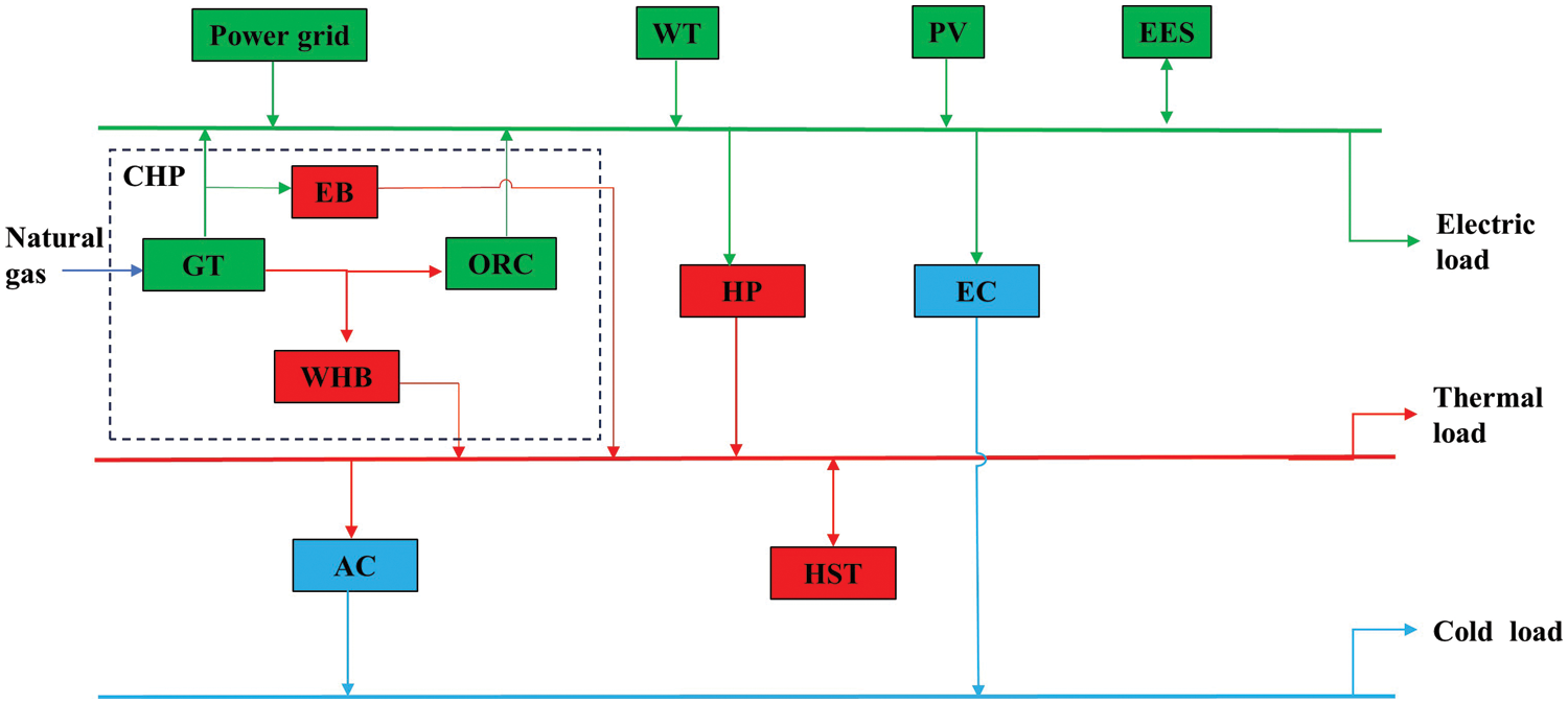
Figure 1: PIES structure diagram

Energy is supplied by wind power (WT), photovoltaic (PV), grid, and natural gas. The power supply equipment mainly consists of gas turbine (GT) and ORC. Heating equipment mainly includes GT, electric boiler (EB), heat pump (HP), and waste heat boiler (WHB). Cooling equipment mainly includes absorption chiller (AC) and electricity chiller (EC). Energy storage equipment mainly includes electric energy storage (EES) and heat storage tank (HST). Within the CHP, it consists of GT, ORC, WHB, and EB.

2.2 Heat Pump Model

{Ph,HP(t)=ηHPPHP(t)PHPmin≤PHP(t)≤PHPmax(1)

where Ph,HP(t) is the HP output thermal power at moment t; PHP(t) is the HP input electric power at moment t; ηHP is the HP conversion efficiency; and PHPmax,PHPmin are the HP input power upper and lower limits, respectively.

2.3 Absorption Chiller Model

{Pc,AC(t)=ηACPAC(t)PACmin≤PAC(t)≤PACmax(2)

where Pc,AC(t) is the AC output cold power at moment t; PAC(t) is the AC input heat power at moment t; ηAC is the AC conversion efficiency; and PACmax,PACmin are the AC input power upper and lower limits, respectively.

2.4 Electricity Chiller Model

{Pc,EC(t)=ηECPEC(t)PECmin≤PEC(t)≤PECmax(3)

where Pc,EC(t) is the EC output cold power at moment t; PEC(t) is the EC input electric power at moment t; ηEC is the conversion efficiency of the EC; PECmax,PECmin are the EC input power upper and lower limits, respectively.

2.5 Energy Storage Equipment Model

From the point of view of energy transfer and conversion, the models of energy storage equipment are similar [23]. Therefore, the EES and HST are expressed in a unified model in this paper.

{Sk(t+1)=Sk(t)+(ηkchaPkcha(t)−Pkdis(t)/ηkdis)Δt0≤Pkcha(t)≤μk(t)Pkcha,max0≤Pkdis(t)≤(1−μk(t))Pkdis,maxSk(1)=Sk(T)Skmin≤Sk(t)≤Skmax(4)

where k denotes the energy type, including electric and thermal energy; Pkcha(t),Pkdis(t) denote that the energy storage device’s charging and discharging power at moment t, respectively; ηkcha,ηkdis denote that the energy storage device’s charging and discharging efficiency, respectively; Pkcha,max,Pkdis,max denote the energy storage device’s upper limit of the charging and discharging power, respectively; Sk(t) denotes storage energy stored by the energy storage device at moment t; μk(t) is a binary variable, when μk(t)=0, it means that energy is discharged at moment t, and when μk(t)=1, it means that energy is charged at moment t; Skmax,Skmin denote the capacity upper and lower limits of the energy storage device; Sk(1),Sk(T) denote the energy stored by the energy storage device from the beginning to the end moment of the system operation, respectively; and Δt is the unit moment.

3  Source-Load Flexible Response Model

3.1 Source Side Flexible Response Model

Traditional CHP units usually consist of the GT and WHB, and generally operate on a heat-to-electricity or heat-to-electricity basis, resulting in a lack of flexible response capability in the event of changes in electricity and thermal loads. In order to optimize the thermoelectric output of CHP to meet the electric and thermal load demands, this paper introduces the ORC, together with the EB and traditional CHP units to construct a CHP thermoelectric flexible response model to realize the thermoelectric flexible response within the system. CHP units can be flexibly adjusted to meet the different demands of electric and thermal loads, which optimizes the system operation.

3.1.1 Gas Turbine Model

{Pe,GT(t)=ηe,GTPGT(t)Ph,GT(t)=ηh,GTPGT(t)PGTmin≤PGT(t)≤PGTmaxΔPGTmin≤PGT(t+1)−PGT(t)≤ΔPGTmax(5)

where Pe,GT(t),Ph,GT(t) denote GT’s electrical and thermal output power at moment t, respectively; PGT(t) denotes GT’s input power at moment t; ηe,GT,ηh,GT are the GT’s efficiency in converting to electrical and thermal energy, respectively; PGTmax,PGTmin are GT’s upper and lower limits of input power, respectively; and ΔPGTmax,ΔPGTmin are GT’s upper and lower limits of hill climbing, respectively.

3.1.2 Organic Rankine Cycle Model

{Pe,ORC(t)=ηORCPORC(t)PORCmin≤PORC(t)≤PORCmaxΔPORCmin≤PORC(t+1)−PORC(t)≤ΔPORCmax(6)

where PORC(t) denotes ORC’s input power at moment t; Pe,ORC(t) denotes ORC’s output electric power at moment t; ηORC denotes ORC’s conversion efficiency; PORCmax,PORCmin are ORC’s upper and lower limits of input power, respectively; and ΔPORCmax,ΔPORCmin are ORC’s upper and lower limits of hill climbing, respectively.

3.1.3 Waste Heat Boiler Model

{Ph,WHB(t)=ηWHBPWHB(t)PWHBmin≤PWHB(t)≤PWHBmax(7)

where PWHB(t) denotes WHB’s input power at moment t; Ph,WHB(t) denotes WHB’s output thermal power at moment t; ηWHB denotes WHB’s waste heat recovery efficiency; PWHBmax,PWHBmin are WHB’s upper and lower limits of input power, respectively.

3.1.4 Electric Boiler Model

{Ph,EB(t)=ηEBPEB(t)PEBmin≤PEB(t)≤PEBmax(8)

where PEB(t) denotes the power input to the EB at moment t; Ph,EB(t) denotes EB’s output thermal power at moment t; ηEB denotes EB’s conversion efficiency; and PEBmax,PEBmin are EB’s upper and lower limits of input power, respectively.

3.1.5 Gas Turbine Electrical and Thermal Power Output Model

GT electrical power flows to the EB and the system, and GT thermal power flows to the WHB and the ORC.

{Pe,GT(t)=PEB(t)+PNET(t)Ph,GT(t)=PWHB(t)+PORC(t)(9)

where PNET(t) is the electric power flowing into the system from GT at moment t.

3.1.6 CHP Electrical and Thermal Power Output Model

{Pe,CHP(t)=PNET(t)+Pe,ORC(t)Ph,CHP(t)=Ph,WHB(t)+Ph,EB(t)(10)

where Pe,CHP(t),Ph,CHP(t) are the electric and thermal heat power output from the CHP at moment t, respectively.

3.1.7 CHP Thermoelectric Output Percentage

In order to reflect the flexibility of CHP thermoelectric output more intuitively, this paper proposes the CHP thermoelectric output percentage to reflect the change of CHP’s thermoelectric output during the scheduling cycle, which is expressed as:

{Xe(t)=Pe,CHP(t)/(Pe,CHP(t)+Ph,CHP(t))Xh(t)=Ph,CHP(t)/(Pe,CHP(t)+Ph,CHP(t))(11)

where Xe(t),Xh(t) are the CHP electrical and thermal output percentage at moment t, respectively.

In order to further reflect the flexible adjustment of the CHP thermoelectric output power according to the load condition, the maximum values Xemax,Xhmax and the minimum values Xemin,Xhmin in Xe(t),Xh(t) are taken to determine the CHP electric output percentage interval Xemin∼Xemax and the CHP thermal output percentage interval Xhmin∼Xhmax, respectively, and the larger the range of the percentage interval, the higher the flexibility of the CHP.

3.2 Load Side Flexible Response Model

Loads can be generally categorized as fixed loads, transferable loads, interruptible loads and substitutable loads. This paper considers transferable loads, interruptible loads and substitutable loads as regulators to participate in the DR, which is expressed as:

Px,Load(t)=Px,Load∗(t)+Px,Loadm(t)+Px,Loads(t)+Px,Loadd(t)(12)

where x denotes the load type, consisting of electric, heat, and cold; Px,Load(t) is the power of x load at time t after DR; Px,Load∗(t) is the power of x load at moment t before DR; and Px,Loadm(t),Px,Loads(t),Px,Loadd(t) are the amount of transferable loads, interruptible loads, and substitutable loads after DR for x load at moment t, respectively.

3.2.1 Transferable Load

{Px,Loadm(t)=Px,Loadm,0(t)+ΔPx,Loadm(t)ΔPx,Loadm(t)=ξxm,in(t)Px,Loadm,in(t)−ξxm,out(t)Px,Loadm,out(t)ξxm,in(t)+ξxm,out(t)=1∑t=1T⁡ΔPx,Loadm(t)=0βxmin≤ΔPx,Loadm(t)≤βxmax(13)

where Px,Loadm,0(t) denotes the transferable load before DR at moment t of x load; ΔPx,Loadm(t) denotes the transferable load participating in DR at moment t of x load; ξxm,in(t),ξxm,out(t) are binary variable, which denote transferable load’s transfer-in and transfer-out parameters at moment t of x load, respectively; Px,Loadm,in(t),Px,Loadm,out(t) denote transferable load’s transfer-in and transfer-out power at moment t of x load, respectively; βxmax,βxmin denote that the transferable loads participate in DR at each moment with upper and lower limits, respectively; and T is the scheduling period.

3.2.2 Interruptible Load

{Px,Loads(t)=Px,Loads,0(t)+ΔPx,Loads(t)0≤ΔPx,Loads(t)≤τxmax(14)

where Px,Loads,0(t) denotes the interruptible load before DR at moment t of x load; ΔPx,Loads(t) denotes the interruptible participating in DR at moment t of x load; τxmax indicates the upper limit of participation in DR for each moment of interruptible load.

3.2.3 Substitutable Load

{Px,Loadd(t)=Px,Loadd,0(t)+ΔPx,Loadd(t)ΔPx,Loadd(t)=ξxd,in(t)Px,Loadd,in(t)−ξxd,out(t)Px,Loadd,out(t)ξxd,in+ξxd,out=1∑t=1TΔPx,Loadd(t)=0(15)

where Px,Loadd,0(t) denotes the substitutable load before DR at moment t of x load; ΔPx,Loadd(t) denotes the substitutable load participating in DR at moment t of x load; ξxd,in(t),ξxd,out(t) are binary variable, which denote substitutable load’s substitute-in and substitute-out parameters at moment t of x load, respectively; Px,Loadd,in(t),Px,Loadd,out(t) denote transferable load’s substitute-in and substitute-out power at moment t of x load, respectively.

4  Stepped Carbon Trading Mechanism

4.1 Carbon Right Initial Quota Model

Unremunerated carbon allowances for the IES are determined through the baseline method. The carbon right allocations in the PIES studied in this paper include both GT and purchased electricity [24]. All of the purchased electricity originates from heat-engine plants. The carbon right initial quota is modeled as follows:

{EIES=Ee,BUY+EGTEe,BUY=δe∑t=1TPe,BUY(t)EGT=δh∑t=1T(δe,hPe,GT(t)+Ph,GT(t))(16)

where Ee,BUY and EGT are the free carbon right allowances for GT and power purchase, respectively; EIES is the total PIES carbon emission allowance; δe and δh are the carbon emission right allowances for generating unit electric power and unit thermal power, respectively; δe,h is the electric and thermal power conversion parameter; Pe,BUY(t) is the power purchase at moment t.

4.2 Actual Carbon Emission Model

The actual carbon emission is modeled as follows:

{EIES,r=Ee,BUY,r+EGT,rEe,BUY,r=∑t=1T(a1+b1Pe,BUY(t)+c1Pe,BUY2(t))EGT,r=∑t=1T(a2+b2Peh,GT(t)+c2Peh,GT2(t))Peh,GT(t)=Pe,GT(t)+Ph,GT(t)(17)

where EIES,r is PIES actual carbon emission; EGT,r is the GT’s actual carbon emission in PIES; Ee,BUY,r is the thermal power generating unit’s actual carbon emission; Peh,GT(t) is the total output power of GT at moment t; a1,b1,c1 are the thermal power generating unit’s carbon emission parameter; a2,b2,c2 are the GT’s carbon emission parameter. Therefore, the actual amount of carbon right traded is:

E=EIES,r−EIES(18)

4.3 Stepped Carbon Emission Trading Model

The stepped carbon trading model is divided into different intervals for different carbon emissions. If the actual carbon emissions are less than the quota at a particular moment, E is negative and IES can sell the extra carbon credits to realize the revenue, while if the actual carbon emissions are more than the quota, E is positive and IES needs to purchase the carbon credits, and the carbon allowance price will increase with the rise of the carbon emissions to limit the carbon emissions [25]. The stepped carbon trading model is:

CCO2={ρE,E≤lρl+ρ(1+θ)(E−l),l<E≤2lρ(2+θ)l+ρ(1+2θ)(E−2l),2l<E≤3lρ(3+3θ)l+ρ(1+3θ)(E−3l),3l<E≤4lρ(4+6θ)l+ρ(1+4θ)(E−4l),4l<E(19)

where CCO2 is the cost of stepped carbon trading, ρ is the base price of carbon trading, l is carbon emission interval length, and θ is the price growth rate.

5  PIES Optimization Model

IES is regarded as an approach to reduce environmental pollution and the use of fossil energy, and the index should reflect its core features at the same time. Therefore, to evaluate the system more comprehensively and scientifically and optimize the system’s equipment output configuration scheme, this paper considers three aspects: economy, energy efficiency, and environment.

5.1 Economic Index

The comprehensive system operation cost f1 includes system operation and maintenance cost Com, income from electricity sales Csell, energy purchase cost Cbuy, stepped carbon trading cost CCO2, DR compensation cost CDR, wind and light abandonment cost Cwp and gas turbine startup and shutdown cost CGT. The expression of the economic evaluation index is:

minf1=Com+Cbuy+CCO2+Cwp+CDR+CGT−Csell(20)

{Com=∑z∈Q∑t=1T(KzPout,z(t))Cbuy=∑t=1Tγ1Pe,BUY(t)+∑t=1Tγ2Pg,BUY(t)Csell=∑t=1Tγ3Pe,SELL(t)Cwp=∑t=1TcwpPwp(t)CDR=∑x∑t=1T(υm|ΔPx,Loadm(t)|+υs|ΔPx,Loads(t)|+υd|ΔPx,Loadd(t)|)CGT=Σt=1T(α(t)(1−α(t+1))fGT+(1+α(t))α(t+1)fGT)(21)

where z is the device type; Q is the set of devices in this paper, Q = {WT, PV, GT, WHB, ORC, EB, HP, EC, AC, EES, HST}; Pout,z(t) is the output power of device z at moment t, and Kz is the operation and maintenance cost per unit of output power of device z; Pg,BUY(t) is the purchased gas quantity at moment t; Pe,SELL(t) is the electricity sold at moment t; γ1,γ2,γ3 are the electricity and gas prices at moment t, respectively; Pwp(t) is wind and solar power abandonment at moment t; cwp is wind and solar power abandonment penalty cost coefficient; υm,υs,υd denote per-unit compensation coefficients after the participation of transferable, interruptible, and substitutable loads in DR, respectively; α(t) denotes the 0-1 variable for the gas turbine start-stop state at moment t, where 0 means stop and 1 means start; fGT is the start-stop penalty cost factor.

5.2 Energy Efficiency Index

Energy is the basis of industrial production, and a high energy utilization rate can save energy. Therefore, this paper adopts the comprehensive energy utilization rate f2 as the energy efficiency evaluation index, and its expression is:

minf2=3600∑t=1T(Pe,Load+Ph,Load+Pc,Load)VgLHV+3600∑t=1TP(22)

where Vg is the volume of natural gas consumed; LHV represents the natural gas calorific value; and P represents system input power.

5.3 Environmental Index

Green and low-carbon energy utilization can achieve the goal of environmental protection and sustainable development. Therefore, this paper takes carbon emission f3 as the environmental evaluation index, and its expression is:

minf3=Ee,BUY,r+EGT,r(23)

5.4 Index Fuzzification

The smaller the operating costs and carbon emissions values, the better their evaluation index; the larger the comprehensive energy utilization rate value, the better their evaluation index. Therefore, the operating costs and carbon emissions are used as decreasing half-Γ-type affiliation function; and the integrated energy utilization is used as increasing half-Γ-type affiliation function.

χ1(f1)={1,f1≤f1minexp⁡(f1min−f1f1min),f1>f1min(24)

χ2(f2)={1,f2>f2maxexp⁡(f2−f2maxf2max),f2≤f2max(25)

χ3(f3)={1,f3≤f3minexp⁡(f3min−f3f3min)f3>f3min(26)

where χ1(f1),χ2(f2),χ3(f3) are the affiliation function of operation cost, comprehensive energy utilization rate and carbon emission, respectively; f1min,f2max,f3min are the optimal value of operation cost, comprehensive energy utilization rate and carbon emission, respectively.

5.5 Comprehensive Evaluation Index Based on ANP

A single evaluation index can only reflect the performance of PIES in one aspect of the economy, energy efficiency, and environment. In order to effectively carry out the comprehensive evaluation of the optimized operation of PIES, a rational and feasible evaluation method is needed to obtain the weighted values of the system’s economic index, energy efficiency index, and environmental index. Although simple and easy to use, the analytic hierarchy process (AHP) is often distorted for complex systems due to over-idealized assumptions [26]. In order to evaluate the complex system more objectively and thoroughly consider the links and constraints between the indicators, this paper adopts ANP to assign weights to the indicators at all levels, thus achieving the green economic evaluation of PIES optimal operation. The expression of the comprehensive evaluation index based on ANP is:

minf=ψ1χ1(f1)+ψ2χ2(f2)+ψ3χ3(f3)(27)

where ψ1,ψ2,ψ3 is the relative weight of the economic, energy efficiency, and environmental index, respectively.

The relative weights of the indexes can be obtained by ANP calculations, which are generally calculated in the following steps:

1)   Compare two by two and construct a judgment matrix. Assuming that the ANP control layer has m criteria, respectively P1,P2,⋯,Pm, and the network layer has N groups of elements, respectively U1,U2,⋯,UN, where the group of elements Ui contains n elements ui1,ui2,⋯,uin(i=1,2,⋯,n) and the group of elements Uj contains v elements, the n elements in Ui are compared two by two, using Ps(s=1,2,⋯,m) as the criterion and element ujl(l=1,2,⋯,v) as the sub-criterion. The evaluation scale is Saaty’s 1 to 9 scale method.

2)   Solve the eigenvectors of the judgment matrix and normalize them to obtain the vector [ωi1jl,ωi2jl,⋯,ωinjl]T. This yields hypermatrix block Wij.

Wij=[ωi1j1ωi1j2⋯ωi1jvωi2j1ωi2j2⋯ωi2jv⋮⋮⋱⋮ωinj1ωinj2⋯ωinjv](28)

W=[W11W12⋯W1NW21W22⋯W2N⋮⋮⋱⋮WN1WN2⋯WNN](29)

3)   Obtain the importance weight of each element to Uj and normalize to obtain the sorting vector [y1j,y2j,⋯,yNj]T, the group of elements unrelated to Uj corresponds to a sub-vector of zero, and obtain the weighting matrix as

Y=[y11y12⋯y1Ny21y22⋯y2N⋮⋮⋱⋮yN1yN2⋯yNN](30)

So the individual word blocks of the weighted hypermatrix W¯ is

W¯ij=yijWij(31)

4)   In order to react to the dependencies between elements, the weighted hypermatrix W¯ needs to be stabilized. Its limit value is

W¯∞=limN→∞1N∑q=1NW¯q(32)

5)   The weight values corresponding to each index are calculated by solving the hypermatrix.

5.6 Constraint Conditions

5.6.1 Renewable Energy Constraints

{0≤PWT(t)≤PWTmax0≤PPV(t)≤PPVmax(33)

where PWT(t),PPV(t) are the output power of WT and PV at moment t, respectively; PWTmax,PPVmax are the upper limit of the output power of WT and PV, respectively.

5.6.2 Electric Power Balance Constraints

{Pe,Load(t)=PWT(t)+PPV(t)+Pe,BUY(t)+Pe,CHP(t)+Pedis(t)−Pe,SELL(t)−PEC(t)−PHP(t)−Pecha(t)0≤Pe,BUY(t)≤B(t)Pe,BUYmax0≤Pe,SELL(t)≤(1−B(t))Pe,SELLmax(34)

where Pe,Load(t) is the power of electric load after DR at moment t; Pe,BUYmax is the upper limit of power purchase at each time; Pe,SELLmax is the upper limit of electricity sale for each time period; B(t) is a binary variable, when B(t)=0 indicates that electricity is sold at moment t, when B(t)=1 indicates that electricity is purchased at moment t.

5.6.3 Thermal Power Balance Constraints

Ph,Load(t)=Ph,CHP(t)+Ph,HP(t)+Phdis(t)−PAC(t)−Phcha(t)(35)

where Ph,Load(t) is the thermal load power after DR at moment t.

5.6.4 Cold Power Balance Constraints

Pc,Load(t)=Pc,EC(t)+Pc,AC(t)(36)

where Pc,Load(t) is the cold load power after DR at moment t.

6  Case Analysis

6.1 Case Setting

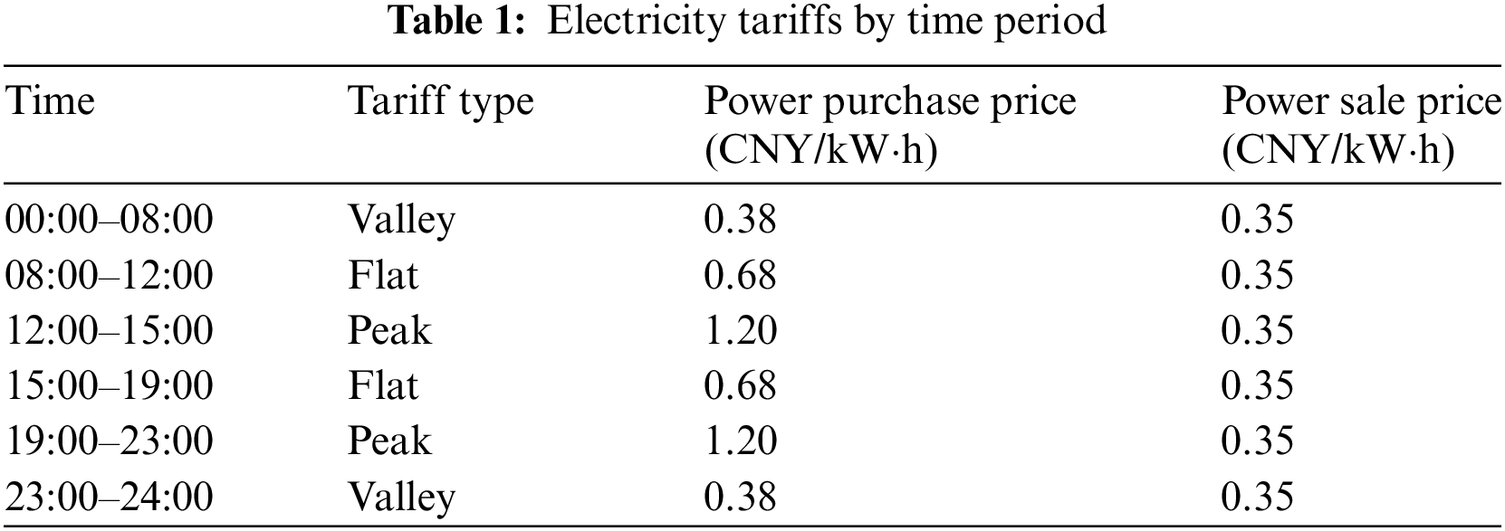
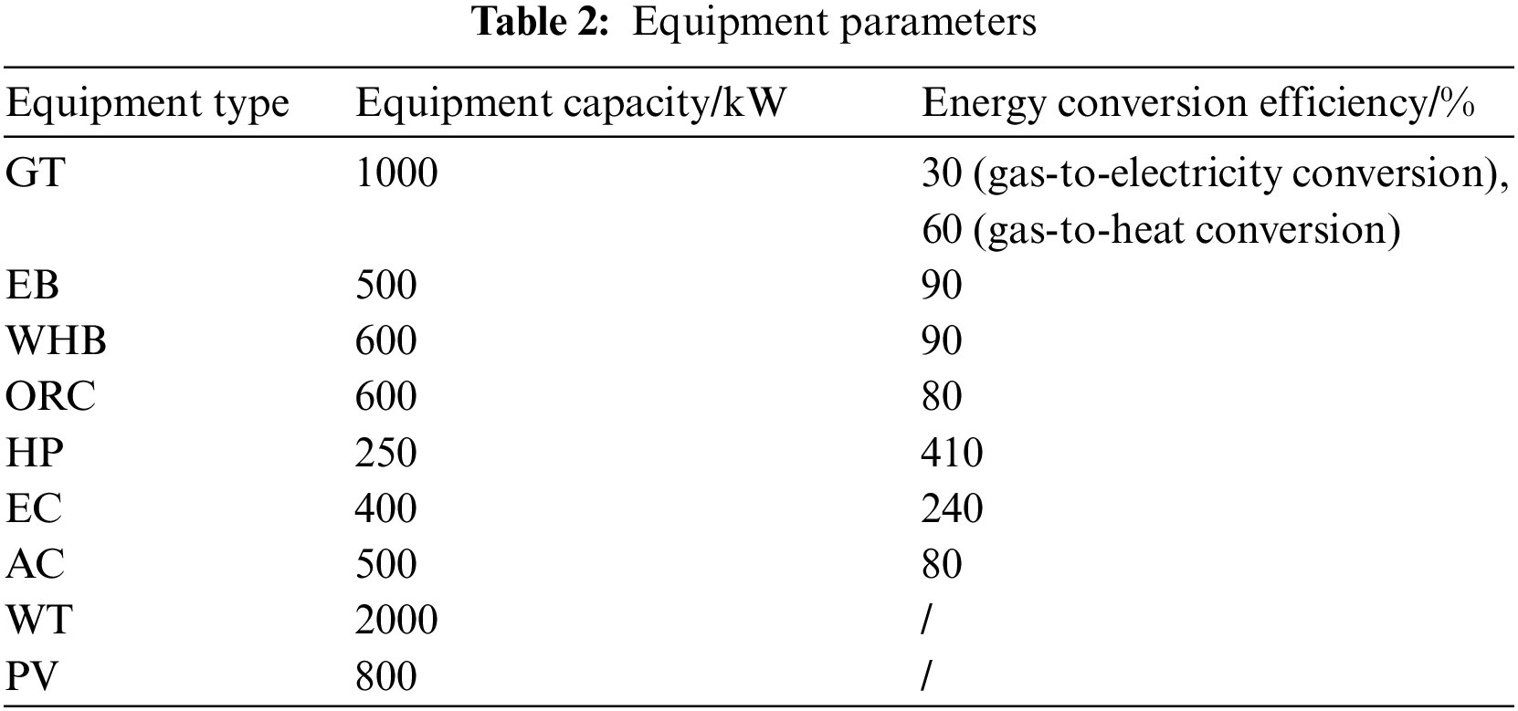
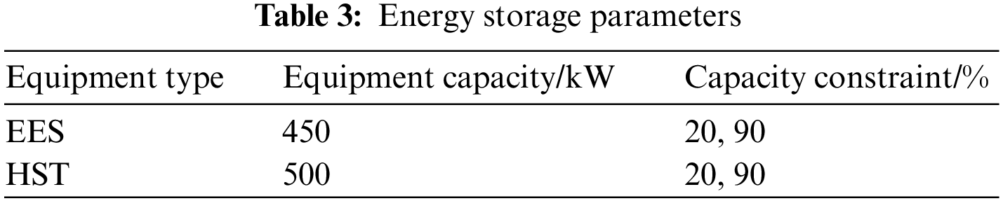
This paper selects a PIES in Northwest China as an example, takes the time step as 1 h and the dispatch cycle as 24 h, and verifies the optimized operation strategy of the IES proposed in this paper. The primary study in this paper is the operation of the proposed flexible response model, so the predicted values of renewable energy output are used. The predicted renewable energy output curves and various load profiles within this PIES are shown in Fig. 2; the hourly electricity prices are shown in Table 1; the parameters of the equipment included in the system are shown in Tables 2 and 3; the parameters of the actual carbon emission model are referenced in the literature [27]; the parameters of the carbon right initial quota model and stepped carbon emission trading model are referred to in the reference [28]; the natural gas calorific value is 9.7 kWh/m3, the unit price of natural gas is 2.55 CNY/m3 [29].

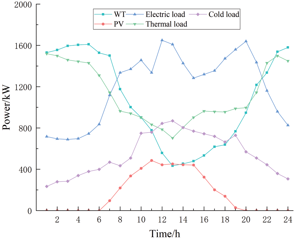
Figure 2: Predicted renewable energy output and individual load curves in PIES

6.2 Optimization Results Analysis

6.2.1 Comparative Analysis of Different Optimization Indexes

In order to compare the differences in scheduling schemes caused by different optimization indexes. Under the source-load flexible response model, the following four optimization indexes are set:

Optimization index 1: Best economic index

Optimization index 2: Best energy efficiency index

Optimization index 3: Best environmental index

Optimization index 4: Best comprehensive index

The results of its operation are analyzed using this as an optimization strategy. The optimization results are shown in Table 4.

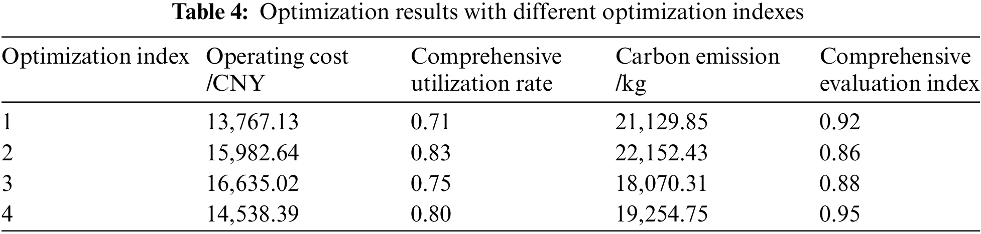
As seen from Table 4, the comprehensive evaluation index for the optimization of economic, energy efficiency, and environmental indicators is smaller than the comprehensive evaluation index for the comprehensive optimization. In order to optimize each index, the value of several other indicators is often reduced, making the value of the comprehensive evaluation index smaller. For comprehensive optimization, although the individual indicators are not optimal, the individual indicators are taken into account to optimize the value of the comprehensive evaluation index. Therefore, the optimal operation scheme based on the comprehensive evaluation index can effectively consider the economy, environmental protection and energy saving of the system operation, and meet the all-round demand of the complex system.

Currently, most IES adopt only the economic index as the only evaluation index. However, Table 4 shows that the environmental and energy benefits of optimization index 1 are poor. Compared with optimization index 4, the environmental benefit of the system is reduced by 8.87%, the energy benefit is reduced by 9%, and the economic benefit is only improved by 5.30%, which is not in line with the requirements of green, low-carbon, and sustainable development. The comprehensive evaluation index based on ANP considers the economy, environment, and energy efficiency, which is more comprehensive and more advantageous than the economic index alone as the only evaluation index.

6.2.2 Analysis of Optimized Scheduling Results

In order to verify the impact of analyzing the source-load flexible response on PIES and the validity of the proposed method, the following four scenarios are set up under the comprehensive evaluation index:

Scenario 1: Fixed thermoelectric ratio output using traditional CHP.

Scenario 2: Fixed thermoelectric ratio output using traditional CHP with IDR consideration.

Scenario 3: Adopt CHP’s flexible response.

Scenario 4: The source-Load flexible response proposed in this paper is used.

The proposed four scenarios are solved, and the system operation results for each scenario are shown in Table 5.

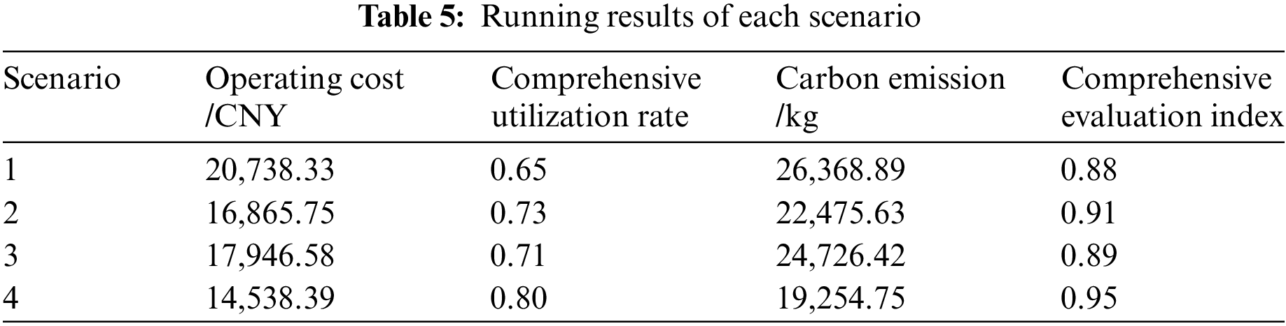
Scenario 3 compared to Scenario 1, the operating cost decreased by CNY 2791.75, i.e., 13.46%; the comprehensive utilization rate increased by 6.00%; and the carbon emissions decreased by 1642.47 kg, i.e., 6.23%. In Scenario 4, compared to Scenario 2, the operating cost decreased by CNY 2327.36, i.e., 13.80%; the comprehensive utilization rate increased by 7.00%; and the carbon emissions decreased by 3220.88 kg, i.e., by 14.33%. It can be seen that source-side flexible response can effectively decrease the system operating costs and carbon emissions, and increase the system energy utilization, and effectively improve the system economy and low-carbon performance.

Scenario 2 compared to Scenario 1, the operating cost decreased by CNY 3872.58, i.e., 18.67%; the comprehensive utilization rate increased by 8.00%; and the carbon emissions decreased by 3893.26 kg, i.e., 14.76%. Scenario 4 compared with Scenario 3, the operating cost decreased by CNY 3408.19, i.e., 18.99%; the comprehensive utilization rate increased by 9.00%; and the carbon emissions decreased by 5471.67 kg, i.e., 22.13%. It can be seen that IDR has good green economic benefits.

In Scenario 4, compared to Scenario 1, the operating cost decreased by CNY 6199.94, i.e., 29.90%; the integrated utilization rate increased by 15.00%; and the carbon emissions reduced by 7114.14 kg, i.e., 26.98%. The comprehensive evaluation index of Scenario 4 is optimal, reaching 0.95, which shows that the source-load flexible response model proposed in this paper is superior to other models, and it can also improve the low-carbon and economic efficiency of the IES.

6.2.3 Source-Load Flexible Responsivity Analysis

Figs. 3–5 show the results of the system’s optimized operation under Scenario 4, and Fig. 6 shows the source-side CHP power output.

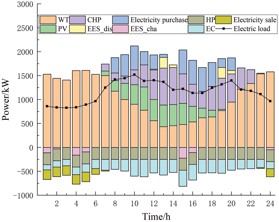
Figure 3: Electric power optimization operation results

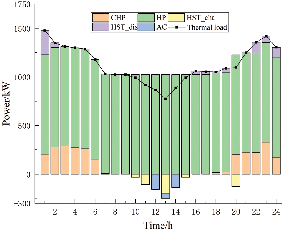
Figure 4: Thermal power optimization operation results

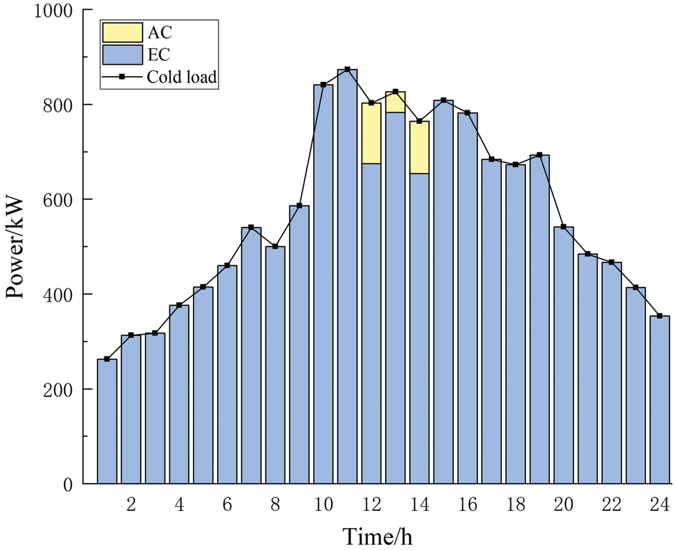
Figure 5: Cold power optimization operation results

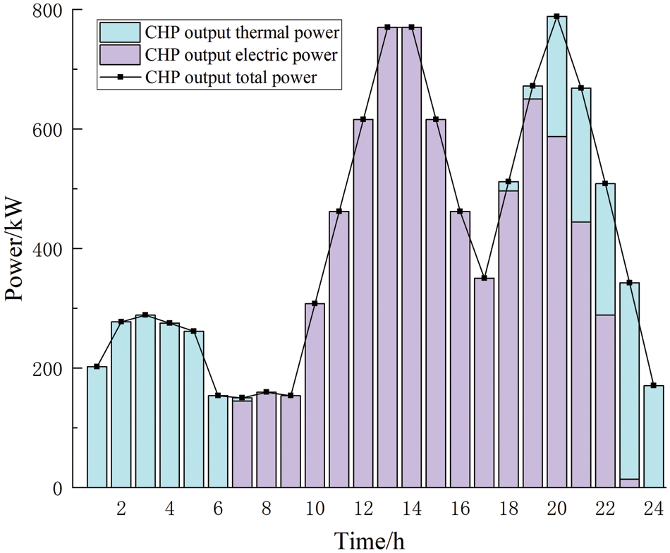
Figure 6: CHP power output diagram

From Figs. 3–5, it can be seen that the 00:00–06:00 time period is the valley time, the electric load is small and the thermal load demand is large, the electric load is fully satisfied by WT, the thermal load is mainly satisfied by HP, CHP mostly carries out the heating, and EC primarily supplies the cold load, and EES carries out the energy storage. The system also sells electricity to the grid due to this period’s abundance of electricity resources. During the 07:00–18:00 time period, the electrical load is large and the thermal load is small, the PV, WT and CHP supply electrical energy simultaneously and also purchase power from the grid, the EES is charged and discharged according to the situation, the HP meets the thermal load demand, the HST is used for thermal storage, the EC and the AC in a flexible way supply the cold load. During the 19:00–24:00 time period, the electrical load first rises and then decreases, the thermal load gradually increases, the PV is no longer supplied At this time, it is mainly supplied by the WT and CHP, the remaining electrical load is satisfied by purchased power and EES discharges, the thermal load is primarily satisfied by the HP and CHP, and the remaining thermal load is satisfied by the HST discharges, and the cold load is satisfied by the EC.

Fig. 6 shows that after the introduction of ORC and EB in CHP, the thermal power output from GT in CHP is provided to ORC for waste heat generation at the higher stage of electrical load, so CHP only outputs electrical power. In the higher thermal load stage, the electrical power output from the GT in the CHP is provided to the EB for heating, so the CHP only outputs thermal power. In other stages, the CHP outputs the corresponding electric and thermal power to meet the load demand according to the system operation. It can be seen that the ratio of the output electric power and thermal power of the source-side CHP can be flexibly adjusted depending on the system’s scheduling requirements.

Table 6 shows the CHP thermoelectric output percentages for Scenarios 1 and 4. It can be seen that the traditional CHP unit in Scenario 1 adopts a fixed thermoelectric ratio output. Its electric and thermal energy output percentage are fixed values, which cannot realize the flexible change of thermoelectric output. The flexible response model proposed in this paper is used in Scenario 4. Its electric and thermal energy output percentage can be varied within 0~100%, which realizes the flexible response of source-side CHP to the load change.

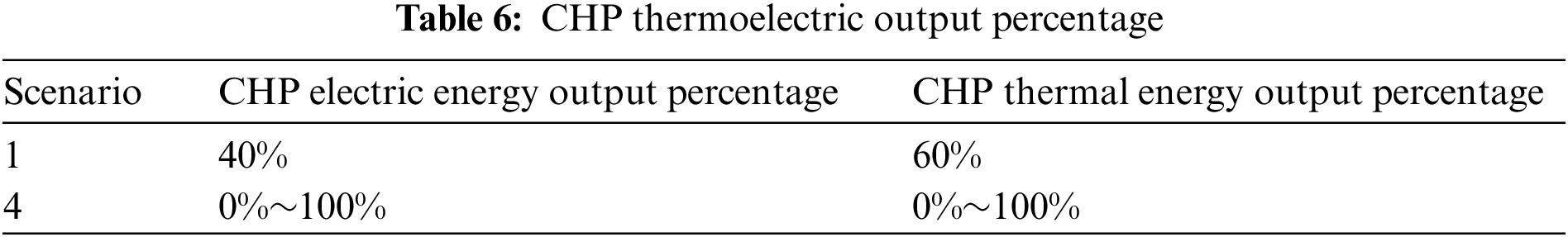
Fig. 7 shows a graph of the change in each load after IDR. From Fig. 7, it is clear that the peak-to-valley difference of electricity, heat, and cooling loads after IDR has decreased by 27.89%, 13.80%, and 4.74%, respectively relative to the pre-IDR, so IDR can effectively smooth out the energy consumption curve. Peak electrical load is reduced, and power purchases from the grid at peak hour tariffs are reduced, thus improving the system’s economy. Increased electrical load in the valley period allows for more renewable energy to be consumed, reducing the output of gas-fired equipment, which in turn reduces the carbon emissions of the system. Each load cuts a portion of its load during its corresponding peak period and raises a portion during the valley period, effectively reducing the peak-to-valley difference of the system and achieving peak shaving and valley filling.

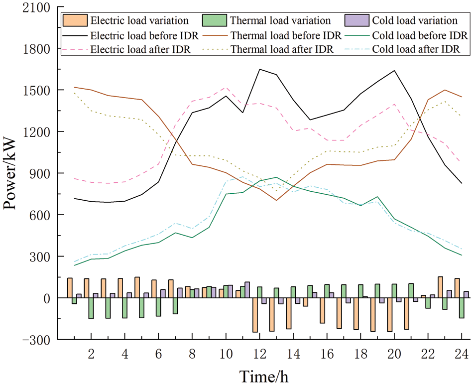
Figure 7: Curve of change in each load after IDR

Fig. 8 shows the system’s renewable energy consumption before and after IDR. From Fig. 8, it can be seen that for Scenario 3 without considering IDR, there is wind and solar abandonment in the 01:00–06:00 and 23:00–24:00 time periods, and for Scenario 4 considering IDR, there is wind and solar abandonment in the 02:00–03:00 time period. From this, it can be seen that considering IDR can adjust the load side energy consumption to reduce reduces the peak energy use and increase the valley energy use, thus increasing the level of renewable energy consumption in the system and reducing the system’s carbon emissions.

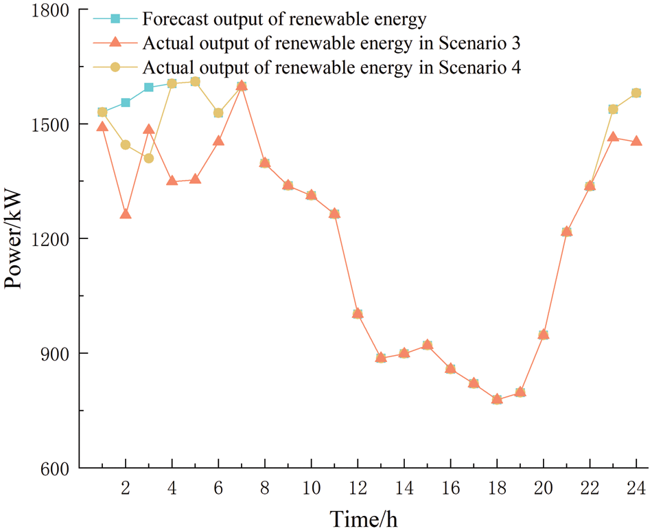
Figure 8: System renewable energy consumption before and after IDR

6.2.4 Sensitivity Analysis of Stepped Carbon Trading

The stepped carbon trading mechanism can effectively limit the carbon emissions of the system operation, and the change of its parameters will also impact the system’s energy saving and carbon reduction effect. Due to the value of the interval length of the stepped carbon trading mechanism, which has the most significant impact on the system operation, the effect of different interval lengths on the system operation cost and carbon emissions is analyzed based on Scenario 4. Fig. 9 shows the effect of interval length change.

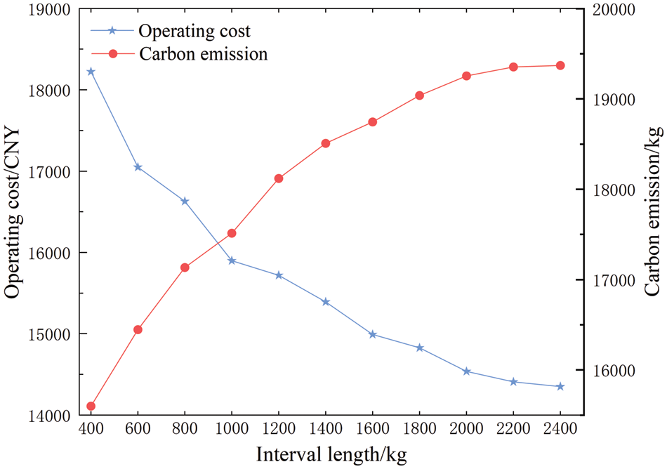
Figure 9: The effect of interval length change

Fig. 9 shows the system operating costs and carbon emissions for interval lengths ranging from 400 to 2400 kg. When the interval length is small, the system must pay a higher cost to offset the high gradient carbon emissions. Hence, a smaller interval length reduces the carbon emissions. Still, the carbon emission cost will be significantly increased, which increases the system operating cost. As the interval length increases, the cost of carbon emissions from the system is reduced, resulting in higher carbon emissions and lower system operating costs. However, as the length of the carbon emission interval continues to increase, the carbon emission capacity reaches the upper limit of the interval under the premise of ensuring that the system operates in a low-carbon economy. The total amount of carbon emissions from the system basically remains unchanged. Thus the operating costs also remain basically unchanged.

7  Conclusion

This study proposes the PIES model of source-load flexible response under the stepped carbon trading mechanism, and thus a comprehensive evaluation index optimization operation model based on ANP is established. The following conclusions are obtained through the analysis of cases:

(1)   The introduction of EB and ORC in the source-side CHP to construct the source-side flexible response model results in a reduction of 13.80% in the operating cost, an increase of 7.00% in the integrated utilization rate, and a decrease of 14.33% in the carbon emissions. The CHP thermoelectric output percentage can be varied from 0% to 100% so that the CHP output power can be flexibly adjusted according to the system’s scheduling needs. The model proposed in this paper effectively enhances the flexibility of PIES operations and reduces system operating costs and carbon emissions.

(2)   Considering IDR on the load side, the peak-to-valley difference between electricity, thermal, and cold loads decreased by 27.89%, 13.80%, and 4.74%, respectively, the operating cost decreased by 18.99%, the integrated utilization rate increased by 9.00%, and the carbon emissions decreased by 22.13%. The model proposed in this paper effectively reduces the peak-to-valley load difference, smooths the energy use curve, and improves the system’s renewable energy consumption level, thereby optimizing the economics of system operation and improving the low-carbon nature of the system.

(3)   By considering the interconnections between indicators through ANP, a comprehensive evaluation index based on ANP is constructed to consider the economy, energy efficiency, and the environment. The comprehensive evaluation index of the model proposed in this paper reaches 0.95, which is superior a single index. The stepped carbon trading mechanism can effectively reduce carbon emissions. By reasonably setting the interval length, it can guide the PIES to operate at the expected carbon emission level while ensuring economy. It can effectively improve the system’s low-carbon performance.

Acknowledgement: None.

Funding Statement: The authors received no specific funding for this study.

Author Contributions: Study conception and design: Xinglong Chen; data collection: He Huang, Qifan Huang, Ximin Cao; analysis and interpretation of results: Xinglong Chen, He Huang; draft manuscript preparation: Xinglong Chen; review and editing: Ximin Cao. All authors reviewed the results and approved the final version of the manuscript.

Availability of Data and Materials: The data presented in this study are available on request from the corresponding author. The data are not publicly available due to patent protection.

Ethics Approval: Not applicable.

Conflicts of Interest: The authors declare that they have no conflicts of interest to report regarding the present study.

References

1. J. Sun, J. Xu, D. Ke, S. Liao, and Z. Ling, “Cluster partition for distributed energy resources in regional integrated energy system,” Energy Rep., vol. 9, no. 284, pp. 613–619, 2023. doi: 10.1016/j.egyr.2023.04.312. [Google Scholar] [CrossRef]

2. M. Yang and Y. Liu, “A two-stage robust configuration optimization framework for integrated energy system considering multiple uncertainties,” Sustain. Cities Soc., vol. 101, no. 3, pp. 105120, 2024. doi: 10.1016/j.scs.2023.105120. [Google Scholar] [CrossRef]

3. V. Stennikov, E. Barakhtenko, and G. Mayorov, “An approach to energy distribution between sources in a hierarchical integrated energy system using multi-agent technologies,” Energy Rep., vol. 9, no. 6, pp. 856–865, 2023. doi: 10.1016/j.egyr.2022.11.117. [Google Scholar] [CrossRef]

4. Z. Zhang and K. S. Fedorovich, “Optimal operation of multi-integrated energy system based on multi-level Nash multi-stage robust,” Appl. Energy, vol. 358, no. 8, pp. 122557, 2024. doi: 10.1016/j.apenergy.2023.122557. [Google Scholar] [CrossRef]

5. A. I. Arvanitidis, V. Agarwal, and M. Alamaniotis, “Nuclear-driven integrated energy systems: A state-of-the-art review,” Energies, vol. 16, no. 11, pp. 4293, May 2023. doi: 10.3390/en16114293. [Google Scholar] [CrossRef]

6. M. A. Mohamed, A. Almalaq, H. M. Abdullah, K. A. Alnowibet, A. F. Alrasheedi and M. S. A. Zaindin, “A distributed stochastic energy management framework based-fuzzy-PDMM for smart grids considering wind park and energy storage systems,” IEEE Access, vol. 9, pp. 46674–46685, 2021. doi: 10.1109/ACCESS.2021.3067501. [Google Scholar] [CrossRef]

7. M. A. Mohamed, T. Jin, and W. Su, “An effective stochastic framework for smart coordinated operation of wind park and energy storage unit,” Appl. Energy, vol. 272, no. 2, pp. 115228, 2020. doi: 10.1016/j.apenergy.2020.115228. [Google Scholar] [CrossRef]

8. R. Sepehrzad, A. S. G. Langeroudi, A. Khodadadi, S. Adinehpour, A. Al-Durra and A. Anvari-Moghaddam, “An applied deep reinforcement learning approach to control active networked microgrids in smart cities with multi-level participation of battery energy storage system and electric vehicles,” Sustain. Cities Soc., vol. 107, 2024. doi: 10.1016/j.scs.2024.105352. [Google Scholar] [CrossRef]

9. H. R. Abdolmohammadi and A. Kazemi, “A benders decomposition approach for a combined heat and power economic dispatch,” Energy Convers. Manage., vol. 71, no. 1, pp. 21–31, 2013. doi: 10.1016/j.enconman.2013.03.013. [Google Scholar] [CrossRef]

10. Z. Luo, J. Wang, H. Wang, W. Zhao, L. Yang and X. Shen, “Optimal scheduling of integrated energy system considering carbon capture and power-to-gas,” (in Chinese), Electr. Power Autom. Equip., vol. 43, no. 12, pp. 127–134, 2023. [Google Scholar]

11. X. Wang et al., “Dynamic modeling and flexible control of combined heat and power units integrated with thermal energy storage system,” Energy Rep., vol. 10, no. 9604, pp. 396–406, Nov. 2023. doi: 10.1016/j.egyr.2023.06.027. [Google Scholar] [CrossRef]

12. Y. Chen, Y. Ma, G. Zheng, Z. Sun, D. Chen and Y. Gao, “Coordinated planning of thermo-electrolytic coupling for multiple CHP units considering demand response,” (in Chinese), Power Syst. Technol., vol. 46, no. 10, pp. 3821–3830, 2022. [Google Scholar]

13. J. Chen, Z. Hu, J. Chen, Y. Chen, M. Gao and M. Lin, “Optimal dispatch of integrated energy system considering ladder-type carbon trading and flexible double response of supply and demand,” (in Chinese), High Volt. Eng., vol. 47, no. 9, pp. 3094–3104, 2021. [Google Scholar]

14. A. Khodadadi, S. Adinehpour, R. Sepehrzad, A. Al-Durra, and A. Anvari-Moghaddam, “Data-driven hierarchical energy management in multi-integrated energy systems considering integrated demand response programs and energy storage system participation based on MADRL approach,” Sustain. Cities Soc., vol. 103, no. 13, pp. 105264, 2024. doi: 10.1016/j.scs.2024.105264. [Google Scholar] [CrossRef]

15. R. Sepehrzad, A. Hedayatnia, M. Amohadi, J. Ghafourian, A. Al-Durra and A. Anvari-Moghaddam, “Two-stage experimental intelligent dynamic energy management of microgrid in smart cities based on demand response programs and energy storage system participation,” Int. J. Electr. Power Energy Syst., vol. 155, no. 3, pp. 109613, 2024. doi: 10.1016/j.ijepes.2023.109613. [Google Scholar] [CrossRef]

16. H. Karimi and S. Jadid, “Multi-layer energy management of smart integrated-energy microgrid systems considering generation and demand-side flexibility,” Appl. Energy, vol. 339, no. 4, pp. 120984, 2023. doi: 10.1016/j.apenergy.2023.120984. [Google Scholar] [CrossRef]

17. J. Datta and D. Das, “Energy management of multi-microgrids with renewables and electric vehicles considering price-elasticity based demand response: A bi-level hybrid optimization approach,” Sustain. Cities Soc., vol. 99, no. 1, pp. 104908, 2023. doi: 10.1016/j.scs.2023.104908. [Google Scholar] [CrossRef]

18. F. Norouzi, H. Karimi, and S. Jadid, “Stochastic electrical, thermal, cooling, water, and hydrogen management of integrated energy systems considering energy storage systems and demand response programs,” J. Energy Storage, vol. 72, pp. 108310, 2023. doi: 10.1016/j.est.2023.108310. [Google Scholar] [CrossRef]

19. A. Ghasemi-Marzbali, M. Shafiei, and R. Ahmadiahangar, “Day-ahead economical planning of multi-vector energy district considering demand response program,” Appl. Energy, vol. 332, no. 1, pp. 120351, 2023. doi: 10.1016/j.apenergy.2022.120351. [Google Scholar] [CrossRef]

20. N. K. Singh, C. Koley, and S. Gope, “A two-stage optimal scheduling strategy of hybrid energy system integrated day-ahead electricity market,” Int. J. Environ. Sustain. Dev., vol. 23, no. 2–3, pp. 231–250, 2024. doi: 10.1504/IJESD.2024.137787 [Google Scholar] [CrossRef]

21. X. Liu, L. Zu, X. Li, H. Wu, R. Ha and P. Wang, “Day-ahead and intra-day economic dispatch of electricity hydrogen integrated energy system with virtual energy storage,” IEEE ACCESS, vol. 11, pp. 104428–104440, 2023. doi: 10.1109/ACCESS.2023.3318737. [Google Scholar] [CrossRef]

22. A. Rigby, M. J. Wagner, and B. Lindley, “Dynamic modelling of flexible dispatch in a novel nuclear-solar integrated energy system with thermal energy storage,” Ann. Nucl. Energy., vol. 204, no. 2, pp. 110534, 2024. doi: 10.1016/j.anucene.2024.110534. [Google Scholar] [CrossRef]

23. T. Zhang, Y. Guo, Y. Li, L. Yu, and J. Zhang, “Optimization scheduling of regional integrated energy systems based on electric-thermal-gas integrated demand response,” (in Chinese), Power Syst. Prot. Control, vol. 49, no. 1, pp. 52–61, 2021. [Google Scholar]

24. J. Wang, J. Xu, S. Liao, L. Sima, Y. Sun and C. Wei, “Coordinated optimization of integrated electricity-gas energy system considering uncertainty of renewable energy output,” (in Chinese), Autom. Elect. Power Syst., vol. 43, no. 15, pp. 2–9, 2019. [Google Scholar]

25. D. Yang, C. Jiang, G. Cai, D. Yang, and X. Liu, “Interval method based optimal planning of multi-energy microgrid with uncertain renewable generation and demand,” Appl. Energy., vol. 277, no. 7, pp. 277–287, 2020. doi: 10.1016/j.apenergy.2018.09.093. [Google Scholar] [CrossRef]

26. L. Zhu, S. Yang, H. Jiang, Z. Wang, X. Bian and L. Ji, “Study on comprehensive evaluation of microgrid planning based on improved ANP,” (in Chinese), Acta Energiae Solaris Sin., vol. 41, no. 3, pp. 140–148, 2020. [Google Scholar]

27. J. Chen et al., “Thermoelectric optimization of integrated energy system considering ladder-type carbon trading mechanism and electric hydrogen production,” (in Chinese), Electric Power Autom. Equip., vol. 41, no. 9, pp. 48–55, 2021. [Google Scholar]

28. H. Yang et al., “Low-carbon economic operation of urban integrated energy system including waste treatment,” (in Chinese), Power Syst. Technol., vol. 45, no. 9, pp. 3545–3552, 2021. [Google Scholar]

29. B. Yun, S. Bai, and G. Zhang, “Optimization of CCHP system based on a chaos adaptive particle swarm optimization algorithm,” (in Chinese), Power Syst. Prot. Control, vol. 48, no. 10, pp. 123–130, 2020. [Google Scholar]