A Two-Layer Optimal Scheduling Strategy for Rural Microgrids Accounting for Flexible Loads

1  Introduction

1.1 Background

Distributed power generation has apparent randomness and volatility, and in recent years, large-scale distributed power supply access to the grid has brought significant challenges to the grid’s scheduling [1,2]. Microgrids can effectively absorb new energy in situ through internal energy exchange and dynamic load regulation by demand-side response, significantly reducing the impact of new energy volatility and uncertainty on the power grid, thus maintaining the stability of the power system [3]. Although the research and application of microgrids are rapidly developing worldwide, the specific challenges and solutions faced in the construction and operation of microgrids vary from country to country and region to region. Especially in China, rural areas present unique requirements and opportunities for microgrid development [4]. In recent years, China has consistently intensified efforts to revamp rural power grids, concurrently advancing the construction of innovative rural microgrids to address challenges such as inadequate power supply capacity and low reliability in rural areas [5–8]. However, the fragile network structure in some rural regions of China, coupled with uncertainties on the source and load sides of microgrids, has significantly constrained the widespread development of microgrids in rural regions [9]. The advancement of science and technology has led to an increasing variety of loads, and flexible loads are one of the effective ways to realize the “interactivity” between supply and demand. Unlike traditional rigid loads, flexible loads, as a kind of schedulable load-side resources, are flexible and variable and will participate in the microgrid scheduling process at a higher frequency [10]. Therefore, accounting for flexible loads in the optimal energy scheduling of rural microgrids is a problem worthy of in-depth research.

1.2 Literature Review

In addition to the inherent flexibility and controllability of microgrids, there are also complex nonlinear economic optimization problems, which pose a significant challenge to the optimal operation of microgrids. Scholars have conducted much research on the optimization of microgrid operations. Yue et al. considered the characteristics and costs of various micropower systems, including generation, pollution control, and standby costs [11]. Rivera et al. used chaotic ant colony algorithms to analyze various micropower systems’ operating costs and environmental management [12]. Dellaly et al., in a meta-analysis, focused on microgrids’ characteristics and investigated each objective’s role [13]. As an objective function, Kweon et al. considered environmental cost, operation cost, and security when optimizing microgrids in islanding mode [14]. Wang et al. developed a model for the optimal allocation of power supply to microgrids in terms of reducing the investment cost and increasing the revenue of power supply [15]. The above studies mainly focus on optimizing the scheduling model or algorithm so that the microgrid obtains the maximum total benefit without considering the impact of load-side resources on the optimal economic operation of the microgrid.

Grover-Silva et al. proposed a day-ahead economic schedule optimization model for microgrid flexible resources, taking into account PV and load uncertainties, which effectively reduces microgrid operating costs by considering PV, power storage, and controllable loads as microgrid flexible resources [16]. Ma et al. conducted a study on the scheduling of shiftable loads and curtailable loads of residential customers in smart grids to minimize the operating costs of the grid [17]. Babaei et al. proposed an optimized scheduling model for multi-microgrids integrating renewable energy sources, schedulable resources, and energy storage systems. The model primarily utilizes schedulable resources to participate in demand-side response, effectively reducing microgrid pollution emissions and pollution management costs [18]. Yang et al. focused on smart communities as the research subject, considering various schedulable residential loads [19]. He established an optimal scheduling model for smart communities participating in demand-side response, aiming to enhance the interests of distribution grid operators. Zou et al. selected typical rural areas abundant in solar energy resources as the research focus [20]. He proposed evaluating the regulating characteristics of shiftable loads and analyzed the impact of these characteristics in rural residential buildings on household photovoltaic consumption. Zhao addressed the issues of the utilization rate of distributed generation (DG) and the operational costs in rural microgrids [21]. He proposed a rural microgrid operation optimization method based on cooperative games, which significantly enhances the economic efficiency of rural microgrid operation and the local consumption of clean energy.

In contrast to urban areas, energy loads in rural regions exhibit more flexible characteristics. Firstly, this is attributed to the fact that rural residents face relatively fewer constraints on working hours, rendering their energy consumption behavior more adaptable compared to urban areas. Secondly, rural areas’ relatively underdeveloped economic status makes residents more sensitive to energy prices [22]. Thoroughly tapping into the adjustable potential of flexible loads in rural areas enables the effective alignment of energy supply and demand and economic optimization and facilitates the efficient utilization of abundant renewable energy resources in rural regions. This is paramount in achieving China’s “double carbon” goal and rural revitalization strategy [23]. Morales et al. proposed a planning methodology for rural microgrids utilizing local renewable resources. Characterizing uncertainties in planning renewable resources and demand introduces an electricity consumption model applied to an isolated rural community. This model can lower energy costs even when user electricity demand increases [24]. Luo et al. meticulously categorized households in a specific rural area based on their energy consumption characteristics [25].

Subsequently, an optimization scheduling model was developed to focus on the economic and comfort objectives, utilizing flexible energy loads in rural areas. Chen et al. formulated an optimal scheduling strategy to minimize the total electricity consumption costs from the user’s perspective [26]. This strategy entails coordinating the operation of air conditioning, electric water heaters, and electric vehicles. Wu established a home energy management system based on the electricity load characteristics of residential areas in southern Anhui, focusing on residences and restaurants [27]. The system employs scheduling optimization to guide users in altering their original electricity consumption patterns, effectively utilizing distributed power generation and reducing electricity costs. The above studies mainly focus on optimizing the cost and comfort of electricity consumption on the user side within the microgrid, failing to fully consider the economics of the supply side of electricity. This limitation may lead to a lack of coordination between the supply and demand sides in the optimization process, which may affect the economic efficiency of the overall system. In addition, low-carbon indicators are critical in the context of the current “double carbon” goal and green development. However, the above studies lack in-depth discussions on controlling carbon emissions and pollutant treatment costs.

In the research on two-layer optimal scheduling of microgrids, Wang et al. used the cost minimization of off-grid microgrids as the upper-layer objective and the revenue maximization of the switching station as the lower-layer objective and used tariffs and charging and discharging schedules as the bridge between the upper and lower layers to achieve a scheduling scheme that maximizes the benefits of the upper and lower layers [28]. Žnidarec et al. proposed a two-layer microgrid energy management system oriented to strategic short-term operation scheduling, and the microgrid operators can develop different operational strategies based on this system [29]. Yang et al. proposed a two-layer optimal scheduling strategy for temperature-controlled and time-shifted capacity microgrids that considers user satisfaction [30]. The above literature focuses on microgrid power generation schedules. Few papers take into account the impact of user demand side response on microgrid economic scheduling. All of them adopt time-of-day tariffs, which makes it difficult to differentiate between the periods when renewable energy sources are left over, and thus go to a better guide for the users to use electricity reasonably.

1.3 Literature Gaps and Motivations

Overall, the current research on microgrid scheduling strategies accounting for flexible loads of residents in rural microgrid research is not comprehensive enough, and there is a lack of research on carefully considering microgrid operation costs and users’ electricity demand. Although existing studies have explored various aspects of microgrid optimization, such as economic scheduling, environmental impacts, and the integration of renewable energy sources, they often need to address rural areas’ unique characteristics and needs. Most research has primarily focused on urban settings or generalized approaches, neglecting rural communities’ distinct, flexible load profiles and economic sensitivities.

In particular, the economic optimization models often emphasize either the supply or demand side without fully integrating both aspects. This lack of coordination can lead to inefficiencies in the overall system performance. Additionally, while some studies have considered demand-side response, they frequently utilize simplified tariff-based approaches that do not adequately reflect the variability and potential of renewable energy sources in rural settings. Moreover, the double carbon goals and the emphasis on green development require a more thorough examination of carbon emissions and pollutant treatment costs, which many current studies still need to address sufficiently.

For China, which has a very vast rural area, it is very meaningful to promote the coverage of microgrid operation mode by effectively utilizing the abundant renewable resources in rural areas to alleviate the costs of electricity consumption by rural residents, especially by utilizing residents’ subjectivity for optimal scheduling of microgrid energy. This gap highlights the need for a more holistic approach integrating supply-side economics and user-centric demand-side management to achieve better economic efficiency and sustainability.

In order to solve the problems of the current research, this paper focuses on the flexible loads in rural areas. It establishes a two-layer scheduling model that considers rural users’ electricity consumption costs and microgrids’ comprehensive operational costs. In the research process, detailed models are developed for shiftable, deferrable, and curtailable loads, along with corresponding comfort models. The two-layer objective functions and constraints are established. The model is solved using the IAGA. Through comparative analysis of simulation results before and after scheduling, the optimization scheduling of microgrids considering flexible loads demonstrates the ability to enhance the stability of energy storage systems and loads and increase the integration of clean energy within microgrids. Additionally, it can effectively balance the operational costs of microgrids and users’ interests.

2  Rural Microgrid Framework

The rural microgrid energy information flow framework is shown in Fig. 1. Microgrids in China’s major rural areas operate in grid-connected mode, exchanging power with the external grid through contact lines [31]. The rural microgrid contains wind turbines (WT), photovoltaic cells (PV), microturbines (MT), storage batteries (BT), rigid loads and flexible loads, which can be categorized into shiftable loads (SL), deferrable loads (DL), curtailable loads (CL) according to the electricity consumption characteristics [32,33]. The microgrid operators adjust the control strategy according to the electricity consumption of rural users and the operation of the microgrid to obtain higher economic benefits.

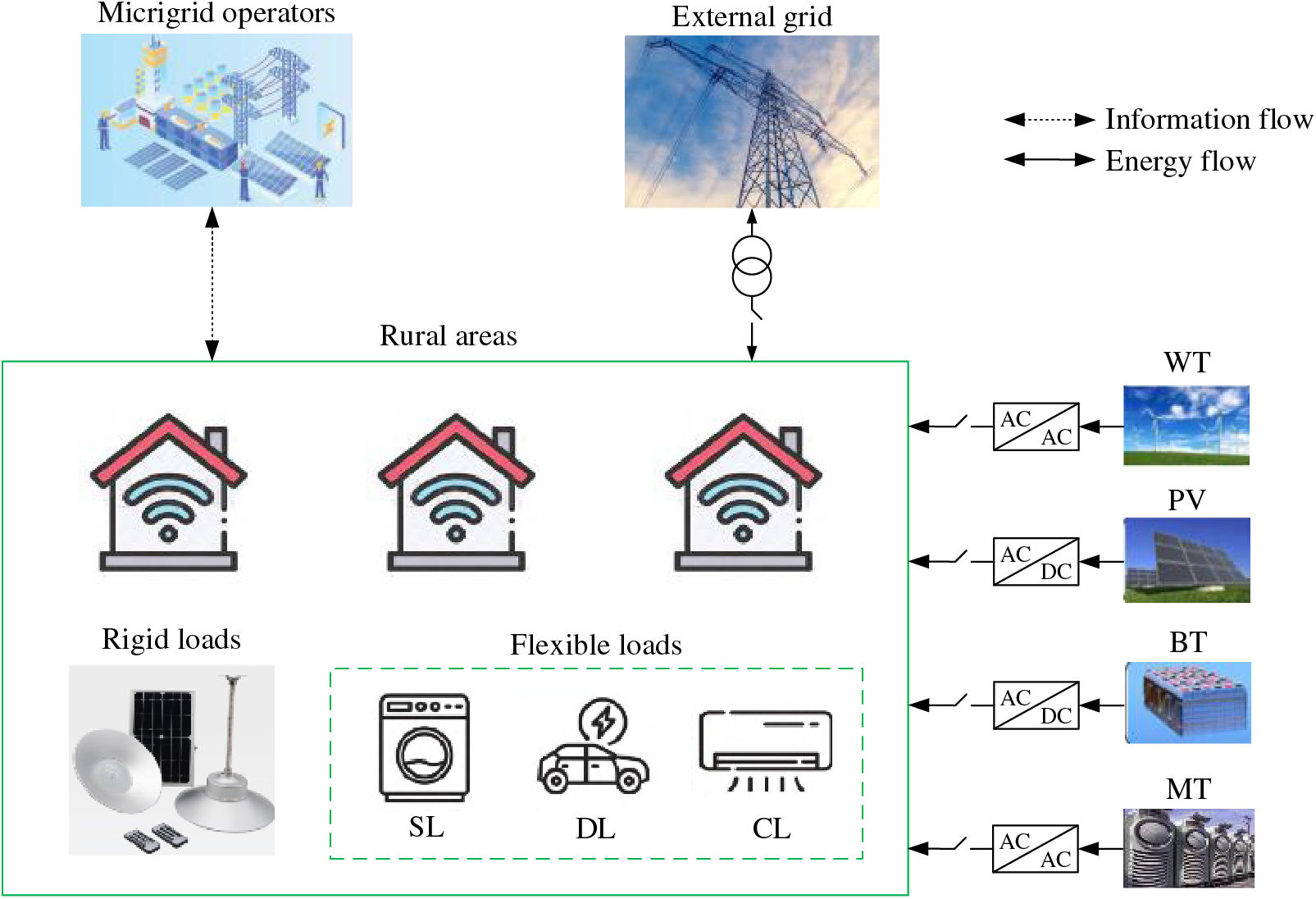
Figure 1: Rural microgrid framework

2.1 Load Modeling for Rural Areas

Loads in rural areas are mainly divided into rigid and flexible loads. Rigid loads have a more significant impact on the lives of rural residents, and this type of load equipment is generally not involved in scheduling and control, such as household lighting equipment, kitchen electricity equipment, etc. The flexible loads refer to the load that can be transferred to other times to participate in the scheduling; its power consumption and power consumption time can be flexible changes, such as air conditioning, electric water heaters, washing machines, etc.; this load can be flexibly scheduled.

2.1.1 SL Model

SL refers to loads for which the usage timing can be shifted from one interval to another within certain permissible limits [34]. The mathematical model for SL can be represented as:

ΔPSL(t)=fSL[t+Δt(ΔδSL(t))]−fSL(t)(1)

∑t=1TΔPSL(t)=0(2)

where ΔPSL(t) is the shiftable power of the load at time step t; ΔδSL(t) is the change in economic performance indicators at time step t; Δt is the shiftable time for loads; fSL(t) is the initial load profile for SL at time step t; T is the scheduling period.

The economic compensation cost for SL is:

CSL=12CprSLΔPSL(t)(3)

where CprSL is the compensation price for SL cell power, and it is set at 0.03 Yuan/kW.

2.1.2 DL Model

DL refers to the loads that can adjust their usage period while keeping the total electricity consumption unchanged. The scheduling of these loads is not constrained by continuity and timing, allowing for flexible adjustments to ensure the equality of the total load within the scheduling period. The mathematical model can be expressed as follows:

ΔPDL(t)=fDL(Δδ(t),PDL(t),eDL(t))−fDL(t)(4)

∑t=1TΔPDL(t)=0(5)

where ΔPDL(t) is the defferable power of the load at time step t; PDL(t) is the base loads power at time step t; PDL(t) is the coefficient of self-defer elasticity at time step t; fDL(t) is the initial load profile for DL at time step t.

The economic compensation cost for DL is:

CDL=12CprDLΔPDL(t)(6)

where CprDL is the compensation price for DL cell power, and it is set at 0.07 Yuan/kW.

2.1.3 CL Model

CL refers to the loads that can adjust the power consumption by a certain magnitude during a specific period. The mathematical model can be expressed as follows:

ΔPCL(t)=fCL(PCL(t),Δδ(t),eCL(t))−fCL(t)(7)

where ΔPCL(t) is the curtailable power of the load at time step t; PCL(t) is the base loads power at time step t; PCL(t) is the coefficient of self-curtail elasticity at time step t; fCL(t) is the initial load profile for CL at time step t.

The economic compensation cost for CL is:

CCL=CprCLΔPCL(t)(8)

where CprCL is the compensation price for CL cell power, and it is set at 0.26 Yuan/kW.

2.2 Microgrid Equipment Modeling

The microgrid equipment model is established by analyzing the grid-connected operation of a typical rural microgrid [35].

2.2.1 WT Model

PWT={0v≤vci or v≥vcoav3+bv2+cv+dvci≤v≤vnPNvn<v<vco(9)

where PWT is the output power of the WT; a, b, c, d are the wind speed parameter settings; vci, vn, vco respectively denote the cut-in wind speed, rated wind speed, and cut-out wind speed.

2.2.2 PV Model

PPV(t)=ηPVSδ(10)

where PPV(t) is the output power of the PV at time step t; ηPV is the PV cell conversion efficiency; S is the PV panel area; δ is the intensity of light radiation.

2.2.3 MT Model

The MT used in the modeling of this paper is Capstone’s C65 micro-gas turbine, which is more commonly used in the market, and its main technical parameters can be referred to as its product specification. The relationship curve between MT output power and power generation efficiency under partial load provided by Capstone C65 micro gas turbine is a polynomial curve fitting through Matlab, and the relationship function between MT power generation efficiency and output power is obtained as follows [36]:

ηMT(t)=0.0753(PMT(t)65)3−0.3095(PMT(t)65)2+0.4174PMT(t)65+0.1068(11)

where ηMT(t) is the efficiency of the MT in generating electricity at time step t; PMT(t) is the output power of the MT at time step t.

The fuel costs formula for MT is:

CMT(t)=∑t=124[C1LHV×PMT(t)ηMT(t)](12)

where CMT(t) is the fuel costs of the MT at time step t; C is the unit price of natural gas; LHV is the low layer heating value of natural gas.

2.2.4 BT Model

EBT(t+1)=EBT(t)−ηCPBT(t)Δt(13)

EBT(t+1)=EBT(t)−PBT(t)ΔtηD(14)

SOC(t+1)={SOC(t)+ηCPBT(t)SOC(t)+ηDPBT(t)(15)

where EBT(t+1), EBT(t) are the storage capacity of the BT at time step t+1, t; PBT(t)<0, PBT(t)>0 are the charging and discharging power of the BT at time step t; ηC, ηD are the charging and discharging efficiencies. Eqs. (13) and (14) represent the BT storage capacity charging and discharging process, and Eq. (15) represents the state of charge (SOC) for energy storage systems.

3  A Two-Layer Optimal Scheduling Model for Rural Microgrids

3.1 A Two-Layer Scheduling Strategy for Rural Microgrids

The rural microgrid scheduling model uses a two-layer scheduling model [37], as shown in Fig. 2. The upper-layer is aimed at minimizing the comprehensive operating costs of the rural microgrid. The decision variables are the flexible load’s compensation costs, the fuel costs of the generation system, the system operation and maintenance costs, the grid interaction costs, and the environmental governance costs, and the grid interaction costs are determined by the price of the microgrid purchasing and selling electricity to the external grid; the lower-layer is aimed at minimizing the total costs of electricity consumption of rural users, and the decision variables are the flexible load’s compensation costs, the users’ comfort level, the amount of electricity consumed, and the price of the electricity purchased. Rural users adjust their electricity consumption plan according to their comfort requirements and purchase electricity prices to reduce electricity expenses [38].

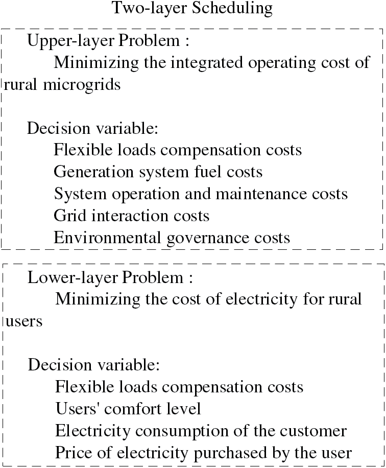
Figure 2: Schematic diagram of two-layer scheduling

In the two-layer optimization scheduling model, the upper-layer focuses on the microgrid’s overall operational costs and efficiency, optimizing from a system perspective. The lower-layer focuses on user-side costs and comfort, optimizing from the user demand perspective. Upper-layer decisions directly impact grid interaction costs, which constitute part of the user’s electricity purchase price, affecting user electricity costs and behavior. When users choose to concentrate electricity usage during low-price periods, the microgrid must adjust its generation and purchasing strategies to accommodate user demand patterns. This model facilitates the interaction between the upper and lower layers, achieving a coordinated optimization of overall system efficiency and individual user needs, thereby enhancing the comprehensive benefits of rural microgrids.

3.2 Rural User Comfort Modeling

3.2.1 SL Comfort Model

The comfort level of SL is associated with the duration of the load’s shifting time; the longer the shifting time, the lower the comfort level for users. This is attributed to the fact that SL typically involves adjustments, switching, or shutting down of electrical equipment, and as the shifting time extends, these alterations may exert a notable impact on the users’ daily lives. The comfort level model of SL is as follows:

USL,i=TSL,i,deTSL,i,de,max=∑t=1TySL,i(t)t−αSL,iβSL,i−αSL,i+1−TSL,i(16)

where USL,i is the users’ comfort level of the ith type of SL; TSL,i,de, TSL,i,de,max are the actual shifting time and the maximum shifting time of the ith type of SL; αSL,i, βSL,i are the start and stop times of the allowed scheduling of the ith type of SL; TSL,i is the total operating time of the ith type of SL; ySL,i(t) is the start-stop variable of the ith type of SL at time step t, which takes the values of 0 and 1.

3.2.2 DL Comfort Model

The total running time of DL remains constant, and its comfort is influenced by the duration of the load deferring time, which can be equivalently referred to as the shifting time. The length of the deferring time directly impacts the response time of the equipment, and any delay in equipment response may lead to a period of discomfort for the users during the deferring process. The comfort level model of DL is as follows:

UDL,i=TDL,i,deTDL,i,de,max=(∑t=αt,iβDL,ixDL,i(t)t−∑t=αt,iαt,i+TDL,i−1t)/TDL,iβDL,i−αDL,i+1−TDL,i(17)

where UDL,i is the users’ comfort level of the ith type of DL; TDL,i,de, TDL,i,de,max are the actual deferring time and the maximum deferring time of the ith type of DL; αDL,i, βDL,i are the start and stop times of the allowed scheduling of the ith type of DL; TDL,i is the total operating time of the ith type of DL; xDL,i(t) is the start-stop variable of the ith type of DL at time step t, which takes the values of 0 and 1.

3.2.3 CL Comfort Model

The comfort level of CL is associated with the operating power of the loads. The longer the loads operate at low power, the lower the users’ comfort level. Because in the low-power operating state, specific electrical devices may fail to reach the expected performance levels. For instance, heating equipment may exhibit diminished heating effects, and refrigeration may experience curtailed cooling or heating effectiveness. These performance variations directly affect the users’ comfort level regarding power consumption. The comfort level model of CL is as follows:

UCL,k=∑t=αCL,kβCL,kxCL,down(t)βCL,k−αCL,k(18)

where UCL,k is the comfort level of the CL operating in stall k; xCL,down(t) is a binary variable for low power operation of the CL at time step t, which takes the values of 0 and 1; αCL,k, βCL,k are the start and stop times of the allowable scheduling of the CL in stall k.

3.3 Objective Function

3.3.1 Lower-Layer Scheduling Objective Function

Lower-layer scheduling aims to minimize the total electricity consumption costs for rural customers. The decision variables are the flexible load’s compensation costs, customer’s comfort, electricity consumption, and power purchase price, and the objective function can be expressed as follows:

{min(∑t=1T(Cprice(t)Pall(t)Δt)+aUall−CFL)Pall(t)=PRL(t)+PSL(t)+PDL(t)+PCL(t)Uall=∑(USL,i+UDL,i+UCL,i)CFL=CSL+CDL+CCL(19)

where URL,k is the power purchase price of the users at time step t; Pall(t) is the total power of the users’ load at time step t; Δt is the scheduling time interval; a is the comfort influence factor, whose larger value indicates that the user’s requirements for comfort are higher; Uall is the total comfort of the rural users’ power equipment; PRL(t), PSL(t), PDL(t), PCL(t) are the power consumption of the rigid loads, SL, DL and CL at time step t; CFL is the flexible loads compensation costs.

3.3.2 Upper-Layer Scheduling Objective Function

The goal of upper-layer scheduling is to minimize the comprehensive costs of rural microgrid operation, which needs to comprehensively consider the economics and environmental protection of microgrid operation [39]. The decision variables include the flexible loads compensation costs, DG’s fuel costs, system operation and maintenance costs, grid interaction costs, and environmental governance costs.

(1)   Economic Costs

The economic costs expression is:

minF1=min(CMT(t)+COM(t)+Cgrid,1(t)+CFL)(20)

COM(t)=∑t=1T[∑i=1N(KOM,iPi(t))](21)

Cgrid,1(t)=∑t=1T[Cbuy(t)Pbuy(t)−Csell(t)Psell(t)](22)

where F1 is the comprehensive costs of microgrid operation; CMT(t) is the system operation and maintenance costs at time step t; Cgrid,1(t) is the grid interaction costs; T is the scheduling cycle; KOM,i is the operation and maintenance coefficient for the ith type of DG; Pi(t) is the output power of the ith type of distributed power supply at time step t; Cbuy(t), Csell(t) are the momentary purchased and sold electricity prices at time step t; Pbuy(t), Psell(t) are the momentary purchased and sold electricity power at time step t.

(2)   Environmental Governance Costs

In order to maintain the ecological balance in rural areas, carbon, and other pollutant emissions need to be minimized during the operation of the microgrid [40], and the environmental governance costs expression is:

minF2=∑t=1T[∑i=1N(∑h=1Mβi,hαhPi(t))](23)

where F2 is the microgrid environmental governance costs; αh is the emission coefficient of the hth type of pollutant emitted by the ith type of DG; αh is the governance costs of the hth type of pollutant.

(3)   Integrated Operating Costs of Microgrid

The integrated operating costs of the microgrid are the sum of the economic costs and the environmental governance costs, which are expressed as:

minF=min(φ1F1+φ2F2)(24)

where F is the integrated operating costs of the microgrid; φ1, φ2 are the proportional coefficients representing the economic costs and environmental governance costs. Considering that both economic viability and environmental sustainability are equally important in the operation of rural microgrid, so set φ1=φ2=0.5.

3.4 Constraint Condition

3.4.1 Microgrid Power Balance Constraint

PL(t)=PPV(t)+PMT(t)+PWT(t)+PBT(t)+Pgrid(t)(25)

where PL(t) is the microgrid demand load power.

3.4.2 DG Output Constraint

PDG,imin(t)≤PDG,i(t)≤PDG,imax(t)(26)

where PDG,imin(t), PDG,imax(t) are the lower and upper limit of the active power of the ith type of distributed power source at time step t.

3.4.3 Interacting Power Constraint

Pgridmin(t)≤Pgrid(t)≤Pgridmax(t)(27)

where Pgridmin(t)<0 indicates that the microgrid provides power to the main grid, Pgridmax(t)>0 indicates that the main grid provides power to the microgrid.

3.4.4 MT Climbing Constraint

Pi,t−1−Pi,t≤RMT-down×T(28)

Pi,t−Pi,t−1≤RMT-up×T(29)

where RMT-down, RMT-up are the minimum and maximum climb rates for the output power of the MT; T is the scheduling cycle.

3.4.5 BT Constraint

EBTmin(t)≤EBT(t)≤EBTmax(t)(30)

SOCmin(t)≤SOC(t)≤SOCmax(t)(31)

∑i=124PBTiγ=0(32)

where EBTmin(t), EBTmax(t) are the lower and upper limits of the output power of the energy storage system at time step t; SOCmin(t) and SOCmax(t) are the lower and upper limits of the energy storage capacity at time step t; γ is the scheduling time period.

3.4.6 Flexible Loads Constraint

(1)   SL Constraint

{PSL(t)=PinSL(t)PoutSL(t)=PinSL(t+σ)=PSL0(t)σ⩽σmax(33)

where PSL0(t), PSL(t) are the power of the load before and after shift at time step t; PinSL(t), PoutSL(t) are the power of the load shifting in and out at time step t; σ is the duration of the load shift; σmax is the maximum limit of the duration of the load shift.

(2)   DL Constraint

{PoutDL(t)=μDL(t)⋅αDL(t)⋅PDL0(t),t∈ϕDL∑t=1TPoutDL(t)Δt=∑t=1TPinDL(t)Δt∑t=1TμDL(t)⩽NmaxDLPDL′(t)=PDL0(t)+PinDL(t)−PoutDL(t)(34)

where PinDL(t), PoutDL(t) are the deferred-in and deferred-out power of the load at time step t; αDL(t) is the defer coefficient of the load at time step t; μDL(t) is the state variable of whether the load participates in the defer or not; PDL0(t), PDL′(t) are the power before and after the defer of the load; ϕDL is the set of time periods during which the load can be deferred; NmaxDL is the maximum number of defers of the load.

(3)   CL Constraint

{ΔPCL(t)=μCL(t)⋅αCL(t)⋅PCL0(t)|αCL(t)−αCL(t−1)|⩽RmaxCLTCL⩽TmaxCLPCL′(t)=PCL0(t)−ΔPCL(t)(35)

where ΔPCL(t) is the curtail power of the load at time step t; αCL(t) is the curtail coefficient of the load at time step t; μCL(t) is the state variable of whether the load participates in the curtailment or not; Rmaxcut is the maximum allowable load curtailment rate coefficient; PCL0(t), PCL′(t) are the power before and after the curtailment of the load; TCL is the length of load curtailment; TmaxCL is the maximum length of load curtailment.

4  Improved Adaptive Genetic Algorithm

4.1 Algorithm Improvement Strategies

Standard Genetic Algorithm (SGA) is an optimization algorithm simulating biological evolution. It simulates the process of biological evolution in nature through selection, crossover, and mutation operations and continuously produces excellent individuals to achieve the purpose of searching for optimal solutions [41]. In the standard genetic algorithm, the population’s characteristics in the evolution process will constantly change; fixed crossover and mutation probability will make the algorithm fall into the local optimal solution, reduce the convergence speed, and solve other problems. Adaptive Genetic Algorithm (AGA) incorporates the algorithm’s adaptive adjustment of crossover and mutation rates into the SGA, which improves the convergence speed of the SGA. However, it also generates a new problem, i.e., the AGA will experience some stagnation in the early stage of the algorithm’s evolution. Therefore, to improve the adaptive adjustment of crossover and mutation rates, solve this stagnation phenomenon, and improve the convergence speed, this paper proposes the IAGA that associates population diversity with crossover and mutation probabilities.

(1)   Coding Method

The coding method determines the representation of genes on an individual as well as the execution of selection, crossover, and mutation operations [42], and the coding method chosen in this paper is as follows:

a−bm[10n10n−1⋯101100]T(36)

where [a,b] is the variable interval; m is the number of variables; n is the dimension of the code.

(2)   Design of the Fitness Function

In genetic algorithms, the evaluation of an individual’s strengths and weaknesses and the determination of the population’s evolutionary direction relies on the individual’s fitness value [43]. The IAGA algorithm assigns crossover probabilities to individuals with different fitnesses, and the fitness function is:

Pc={k1(fmax−f′)fmax−f¯f′⩾f¯k2f′<f¯(37)

where Pc is the individual adaptive crossover rate; k1, k2 are the crossover coefficient, which generally makes the direct crossover where the fitness is less than the mean, so k2=1; fmax is the maximum individual fitness of the population; f¯ is the mean fitness.

(3)   Mutation Optimization

The mutation operation enhances the diversity of the population by modifying specific genes of the parent to generate offspring. This helps to some extent in avoiding local optimization situations [44]. The IAGA algorithm determines the mutation rate based on the individual fitness of the population, which is specified as:

Pm={k3(fmax−f)fmax−f¯f⩾f¯k4f<f¯(38)

where Pm is the individual adaptive mutation rate; k3, k4 are the coefficient of variation, which generally causes individuals whose fitness is less than the mean to mutate directly, so k4=1.

Selection and iteration refer to choosing individuals with high fitness from each optimization result as the initial population for the subsequent optimization. The crossover, mutation, and selection process is repeated to complete the optimization. IAGA is employed to solve the microgrid’s established two-layer optimization scheduling model. The specific process of IAGA is illustrated in Fig. 3.

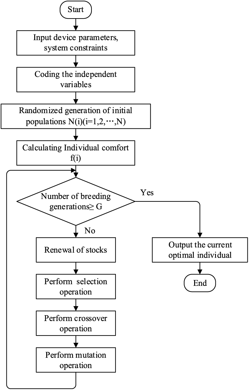
Figure 3: IAGA flowchart

4.2 Algorithm Performance Analysis

In order to comprehensively compare the optimization performance of SGA, AGA, and IAGA, four classical test functions with a certain complexity are selected for testing, and all three algorithms use binary coding and the same selection strategy. All three algorithms use binary coding and the same selection strategy. In the experiment, the population size is 30, and the maximum number of evolutionary generations is 100. The experimental results obtained after running each of the four test functions for 100 times are as follows:

From the results in Tables 1 and 2, it can be seen that although AGA has fast convergence speed, its evolutionary ability is poor, and it tends to fall into the local optimal solution prematurely; the average convergence result of SGA is slightly higher than that of AGA, but its convergence speed is inferior to that of AGA and IAGA, and IAGA proposed in this paper is stronger than the previous two algorithms in its ability to find the global optimal solution, and at the same time, it has a faster convergence speed.

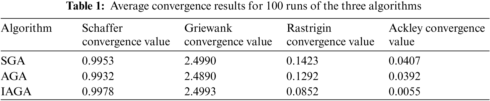
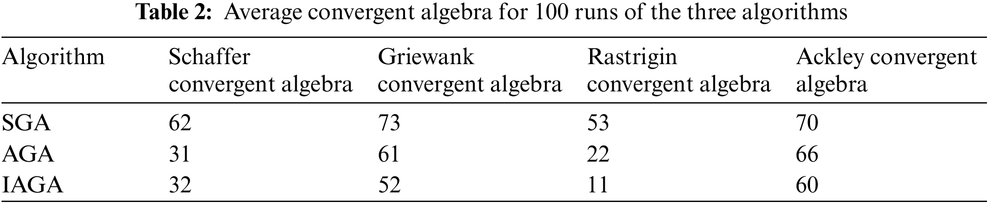
Fig. 4 shows the performance comparison of SGA, AGA, and IAGA in searching for maximum adaptation under four classical test functions performance comparison of searching for maximum fitness under four classical test functions.

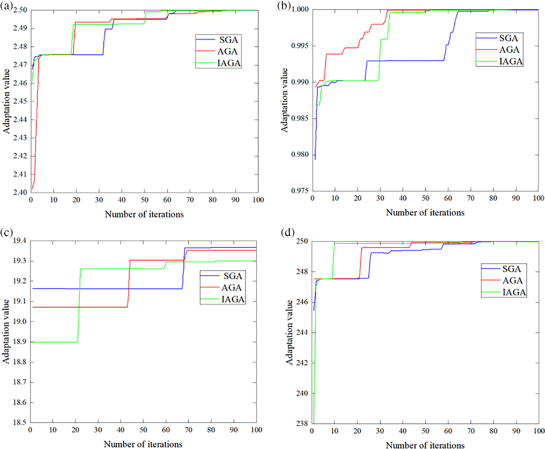
Figure 4: SGA, AGA, IAGA retrieve maximum adaptive performance: (a) Schaffer function, (b) Griewank function, (c) Rosenbrock function and (d) Ackley function

As can be seen from the figure, SGA and AGA are prone to stagnation at the beginning of the convergence process. At the same time, SGA adopts a fixed crossover rate and mutation rate, so when there are more individuals with a higher degree of concentration in the population, it is difficult for SGA to let these individuals crossover and mutate. Then, it cannot jump out of the locally optimal solution. AGA has improved the convergence effect by adapting the crossover and mutation rates. However, it did not avoid the problem of quickly falling into the local optimal solution at the early stage of evolution. On the other hand, the IAGA proposed in this paper solves the problem that the algorithm can easily fall into the local optimal solution at the early stage. By comparing the proximity between the average and maximum fitness and adjusting the crossover and mutation rates, the algorithm can converge well and avoid local optimal solutions.

5  Simulation Analysis

5.1 Parameters of the Algorithm

This paper selects a grid-connected microgrid in a rural area of central China for example analysis, with a test time step of 0.5 h and an operation cycle of 24 h. The number of households in rural areas selected for the example is 1000. The DG operation parameters, pollutant emission coefficient and governance costs, time division and electricity purchase and sale prices, BT parameters, and flexible loads parameters of the microgrid system in this rural area are shown in Tables 3–7. The average output prediction curves for the next day for the rigid loads in this area and the PV and WT are shown in Figs. 5 and 6. IAGA is applied to solve the algorithm in a Matlab environment.

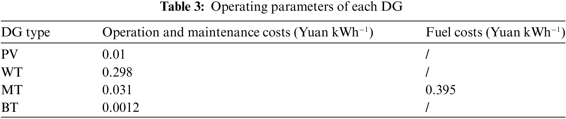
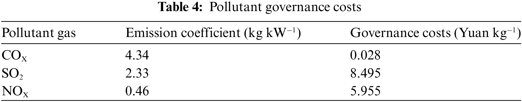
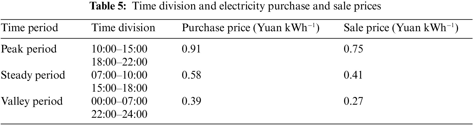
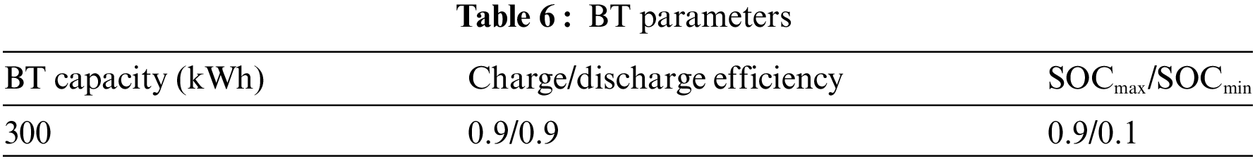
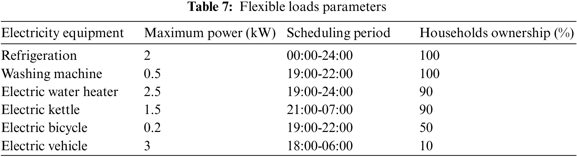
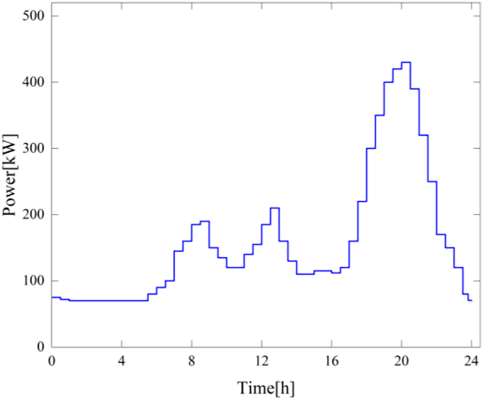
Figure 5: Rigid loads output prediction curve

Figure 6: PV and WT output prediction curves

In order to verify the effectiveness of the two-layer scheduling model considering flexible loads in the optimal scheduling of rural microgrids, the following two scenarios are set up in this paper for comparison: the optimal scheduling scenario of rural microgrids with the two-layer scheduling model considering flexible loads (After schedule) and the scenario before performing optimal scheduling (Before schedule, using predicted data).

5.2 Analysis of Changes in Energy Storage Systems before and after Schedule

The power fluctuations and SOC changes of individual BT storage units before and after the schedule are shown in Fig. 7.

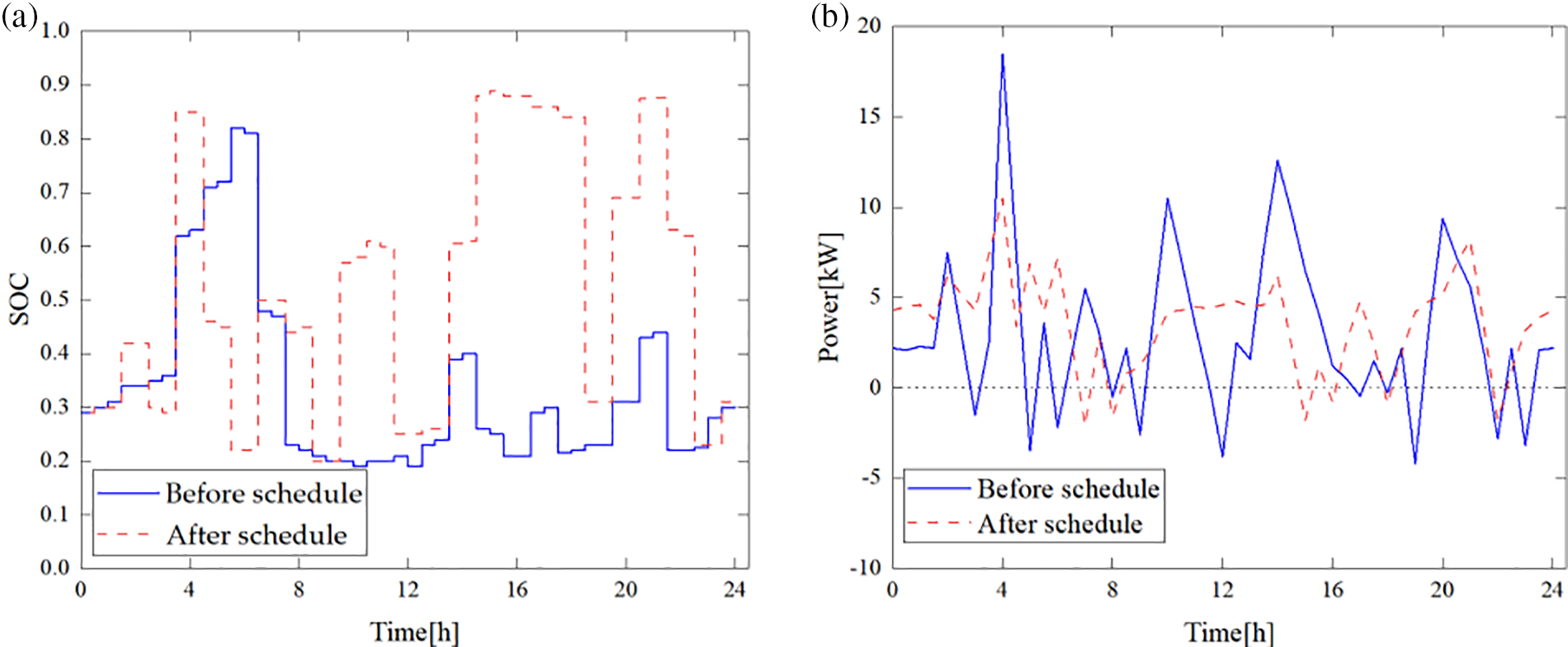
Figure 7: Changes in energy storage systems: (a) BT SOC changes and (b) BT power fluctuations

The energy storage device charges and stores power during the valley period and discharges to supplement the microgrid power during the peak period when the electricity price is higher. As can be seen from the figure, the SOC value of the optimal scheduling model for rural microgrids considering flexible loads is significantly higher than the value before schedule in most of the time, especially in the interval of 14:00–23:00, where the peak SOC value reaches 0.89, which is higher than the peak SOC value of 0.82 before schedule. After the schedule, the charging and discharging frequency of a single BT storage device is minor, and the daily charging and discharging times are 12, much lower than the number of 22 times before the schedule. This approach not only saves the costs of microgrids but also rationally optimizes the configuration scheme and improves the flexibility and stability of rural microgrids’ power supply.

5.3 Analysis of Residential Electricity Load before and after Schedule

In rural microgrid systems, flexible loads are considered in the microgrid energy optimization scheduling process due to their adjustability. Before and after the implementation of the scheduling strategy, the residential electricity load in this rural area is illustrated in Fig. 8, with daily load parameters detailed in Table 8.

Figure 8: Residential electricity load before and after schedule

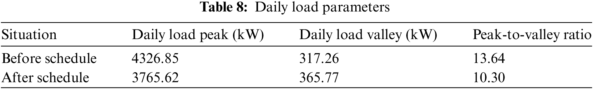
In Fig. 8, the frequency of repeated charging and discharging of the BT significantly decreases after the schedule. The BT utilizes charging and discharging to smooth out load fluctuations. From the comparison of residential electricity load before and after schedule, it is evident that before schedule, the peak of residential electricity consumption in the rural area is concentrated between 18:30–20:30, with daily peak and valley values of 4326.85 and 317.26 kW. The peak-to-valley ratio is 13.64, indicating a significant disparity in daily consumption peaks and valleys for users in the rural area before schedule. After incorporating flexible loads into the two-layer optimization schedule of the microgrid, the peak of residential electricity consumption shifts to 4:30–6:30 on the same day. The daily peak and valley values are 3765.62 and 365.77 kW, with a peak-to-valley ratio of 10.3. These metrics show a noticeable decrease compared to the conditions before schedule.

5.4 Analysis of Clean Energy Output before and after Schedule

Fig. 9 shows the WT and PV output in the microgrid in this rural area before and after the schedule.

Figure 9: Changes in (a) WT output and (b) PV output

As can be seen from the figure, compared with the scenario before optimized scheduling (prediction output curves), there is a considerable degree of improvement in both PV and wind power output after scheduling. In predicting the output of PV and WT for the next day, the output does not reach the maximum power output level due to wind and light abandonment, and the lack of system flexibility and stability causes the problem of power waste and energy dissipation. Flexible loads can adjust the time and intensity of power consumption according to the output of distributed power sources, which can increase the power demand during peak hours and avoid the phenomenon of light and wind abandonment due to excess power supply. The flexible loads’ valley shaving and peak filling function can smooth the power demand curve, allowing distributed power sources to connect to the grid more stably and increase their power utilization. In addition, the flexible load scheduling model quickly responds to fluctuations in distributed power sources by adjusting supply and demand in real time, which enhances the system’s flexibility and reduces the scheduling pressure due to changes in power output. Combined with the energy storage system, it stores energy during peak power output. It releases energy during trough periods, smoothing power output and improving grid stability, effectively solving the problem of distributed power output uncertainty. Therefore, it can be concluded that after the introduction of the two-layer optimal scheduling model considering flexible loads, the loads can better coordinate the relationship between load energy use and distributed power output, which effectively improves the clean energy consumption rate and provides a solution to the problem of distributed energy output uncertainty.

5.5 Economic Analysis of a Two-Layer Scheduling Model

In solving the two-layer optimal scheduling model, it is necessary to comprehensively consider the costs of electricity consumption of rural users and the integrated operating costs of rural microgrids, so three scenarios (adding the single-layer scheduling scenario based on the previous paper) are set up to analyze the results economically. One is the scenario before optimal scheduling is carried out, the second is a single-layer scheduling scenario that only considers the electricity consumption costs of rural users and does not consider the integrated operation costs of rural microgrids, and the third is a scenario that adopts the two-layer optimal scheduling strategy for rural microgrids designed in this paper that considers flexible loads. In the scenario that only considers the integrated operating costs of the microgrid and does not consider the electricity costs of rural users, the rural users have lower comfort and higher electricity costs, so the scenario is not set. The electricity consumption and microgrid operation costs in different scenarios are shown in Table 9.

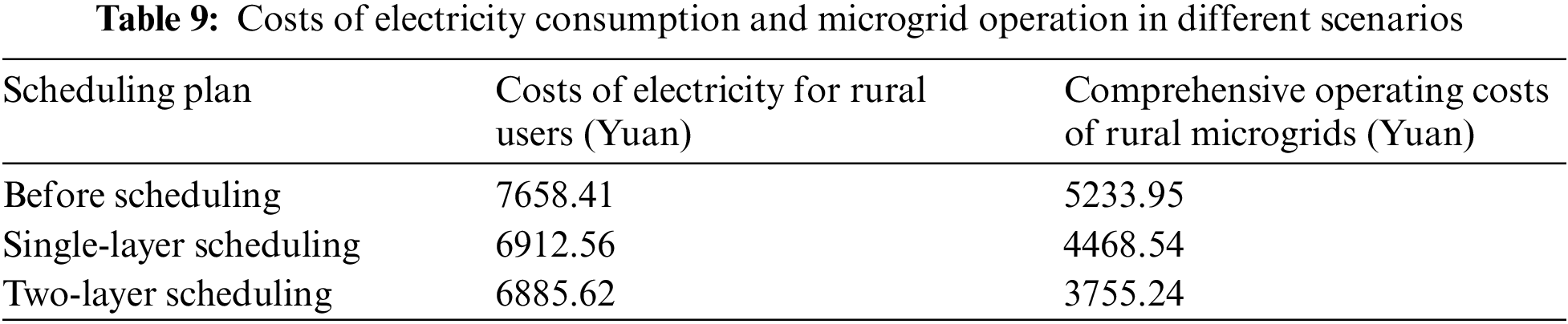
The data in the table indicates that the two-layer scheduling model established in this paper, considering flexible loads, demonstrates significant reductions in rural user electricity costs and integrated operating costs of rural microgrids compared to the scenario before scheduling, affirming the economic viability of the scheduling strategy. Compared to single-layer scheduling, the two-layer scheduling strategy, while leading to a slight increase in users’ electricity costs, results in a substantial decrease of 713.3 Yuan in the integrated operation costs of the microgrid. This economic advantage is noteworthy, as it balances microgrid operation costs and users’ interests.

6  Conclusion

This paper proposes a two-layer optimal scheduling strategy for rural microgrids accounting for flexible loads in light of the operating characteristics of microgrids in rural areas and users’ electricity demand. The following conclusions are drawn through a comparative analysis of results before and after the schedule:

(1) By analyzing the changes in the parameters of the energy storage system before and after the schedule, the SOC value of the optimal scheduling model for rural microgrids accounting for flexible loads is significantly higher than before the schedule. The number of times charging and discharging the BT is less, which can effectively save microgrids’ operation costs and improve rural microgrids’ flexibility and stability.

(2) Aiming at the outstanding characteristics of flexible loads in rural areas, the flexible loads are taken into account in the energy optimization scheduling process of rural microgrids, and by analyzing the loads of rural residents before and after the schedule, the scheduling strategy proposed in this paper can effectively reduce the peak-to-valley difference of loads, slow down the fluctuation of distributed energy sources, and enhance the stability of the power system.

(3) For the renewable energy-rich rural areas, the two-layer optimal scheduling model with flexible loads enhances distributed power utilization, smoothing output fluctuations. Coupled with energy storage, it improves grid stability by storing energy during peak output and releasing it during low demand, effectively managing distributed energy uncertainties.

(4) By comparing and analyzing the costs of electricity consumption of rural users and the operating costs of the microgrid under three scenarios: before scheduling, single-layer scheduling, and two-layer scheduling, the two-layer scheduling model proposed in this paper is more economical, and it can take into account the interests of the microgrid operator and users.

(5) The scheduling strategy proposed in this paper has better application scenarios in actual microgrids in rural areas. Through reasonable modeling and optimal scheduling, rural microgrids can respond positively to problems of load fluctuation, renewable resource waste, rural users’ sensitivity to electricity costs, and high comprehensive operating costs, thus realizing green, sustainable, and user-satisfied energy management.

In this paper, the study of optimal energy scheduling in rural microgrids considers only the typical day user electricity consumption and DG output. The electricity consumption of different seasons and user types is not considered. Therefore, the next step of the work will be to establish the scheduling model of different user types under different time conditions and develop the corresponding control strategies.

Acknowledgement: All authors acknowledge the support and cooperation of their respective institutions.

Funding Statement: The authors received no specific funding for this study.

Author Contributions: The authors confirm their contribution to the paper as follows: study conception and design: Guo Zhao, Chi Zhang, mainly discuss the problems of current research and propose a two-layer optimal scheduling model that integrates the integrated operating costs of microgrids and the costs of electricity consumption of users, and conceptualizes the research lineage of the paper; data collection: Chi Zhang, Qiyuan Ren, relying on the group’s rural microgrid project to travel to the field for data collection, obtaining simulation case parameters, and verifying the validity of the scheduling model; analysis and interpretation of results: Guo Zhao, Chi Zhang, mainly based on the results of simulation data, to verify the validity of the constructed two-layer scheduling model, to compare with other researches, and to highlight the innovativeness of the article; draft manuscript preparation: Chi Zhang. All authors reviewed the results and approved the final version of the manuscript.

Availability of Data and Materials: All data are presented in the paper.

Ethics Approval: Not applicable.

Conflicts of Interest: The authors declare that they have no conflicts of interest to report regarding the present study.

References

1. S. K. Sahoo, A. K. Sinha, and N. K. Kishore, “Control techniques in AC, DC, and hybrid AC-DC microgrid: A review,” IEEE J. Emerg. Sel. Topics Power Electron., vol. 6, no. 2, pp. 738–759, Dec. 2017. doi: 10.1109/JESTPE.2017.2786588. [Google Scholar] [CrossRef]

2. Z. H. Jiang, J. Y. Tu, S. C. Liu, J. Peng, and G. Ouyang, “Research on coordinated development and optimization of distribution networks at all levels in distributed power energy engineering,” Comput. Mater. Contin., vol. 120, no. 7, pp. 1655–1666, May 2023. doi: 10.32604/ee.2023.026981. [Google Scholar] [CrossRef]

3. R. L. Deng, Z. Y. Yang, M. Y. Chow, and J. M. Chen, “A survey on demand response in smart grids: Mathematical models and approaches,” IEEE Trans. Ind. Inform., vol. 11, no. 3, pp. 570–582, Mar. 2015. doi: 10.1109/TII.2015.2414719. [Google Scholar] [CrossRef]

4. H. Z. Yuan, H. H. Ye, Y. T. Chen, and W. Y. Deng, “Research on the optimal configuration of photovoltaic and energy storage in rural microgrid,” Energy Rep., vol. 8, pp. 1285–1293, Nov. 2022. doi: 10.1016/j.egyr.2022.08.115. [Google Scholar] [CrossRef]

5. J. S. Han, L. Zhang, and Y. Li, “Spatiotemporal analysis of rural energy transition and upgrading in developing countries: The case of China,” Appl. Energy, vol. 307, Feb. 2022, Art. no. 118225. doi: 10.1016/j.apenergy.2021.118225. [Google Scholar] [CrossRef]

6. E. I. C. Zebra, H. J. van der Windt, G. Nhumaio, and A. P. C. Faaij, “A review of hybrid renewable energy systems in mini-grids for off-grid electrification in developing countries,” Renew. Sustain. Energy Rev., vol. 144, Jul. 2021, Art. no. 111036. doi: 10.1016/j.rser.2021.111036. [Google Scholar] [CrossRef]

7. F. Azeem et al., “A novel automated demand response control using fuzzy logic for islanded battery-operated rural microgrids,” IET Renew. Power Gener., vol. 17, no. 7, pp. 1797–1811, May 2023. doi: 10.1049/rpg2.12713. [Google Scholar] [CrossRef]

8. H. Q. Lu, X. Y. Wu, W. Zhou, and F. S. Huang, “Distribution network reactive power optimization considering photovoltaic reactive power zonal pricing,” (in Chinese), Guangdong Power, vol. 33, no. 1, p. 8, Jan. 2020. doi: 10.3969/j.issn.1007-290X.2020.001.008. [Google Scholar] [CrossRef]

9. Z. Yang, J. J. Hu, X. Ai, J. C. Wu, and G. Y. Yang, “Transactive energy supported economic operation for multi-energy complementary microgrids,” IEEE Trans. Smart Grid, vol. 12, no. 1, pp. 4–17, Jul. 2020. doi: 10.1109/TSG.2020.3009670. [Google Scholar] [CrossRef]

10. L. J. Yang, K. T. Huang, X. L. Kong, X. J. Lv, and H. J. Guo, “Capacity optimization configuration of grid-connected microgrid system considering flexible load,” Acta Energy Sol. Sin., vol. 42, no. 2, pp. 309–316, Feb. 2021. doi: 10.19912/j.0254-0096.tynxb.2018-0780. [Google Scholar] [CrossRef]

11. Y. W. Yue, Y. Peng, and D. C. Wang, “Deep learning short text sentiment analysis based on improved particle swarm optimization,” Electronics, vol. 12, no. 19, Oct. 2023, Art. no. 4119. doi: 10.3390/electronics12194119. [Google Scholar] [CrossRef]

12. M. M. Rivera, C. Guerrero-Mendez, D. Lopez-Betancur, and T. Saucedo-Anaya, “Dynamical sphere regrouping particle swarm optimization: A proposed algorithm for dealing with PSO premature convergence in large-scale global optimization,” Mathematics, vol. 11, no. 20, Oct. 2023, Art. no. 4339. doi: 10.3390/math11204339. [Google Scholar] [CrossRef]

13. M. Dellaly, S. Skander-Mustapha, and I. Slama-Belkhodja, “Optimization of a residential community’s curtailed PV power to meet distribution grid load profile requirements,” Renew. Energy, vol. 218, no. 5, Dec. 2023, Art. no. 119342. doi: 10.1016/j.renene.2023.119342. [Google Scholar] [CrossRef]

14. J. Kweon, H. Jing, Y. Li, and V. Monga, “Small-signal stability enhancement of islanded microgrids via domain-enriched optimization,” Appl. Energy, vol. 353, no. 3, Jan. 2024, Art. no. 122172. doi: 10.1016/j.apenergy.2023.122172. [Google Scholar] [CrossRef]

15. L. M. Wang, J. C. Liu, C. G. Tian, G. Q. Li, and W. Z. Wei, “Capacity optimization of hybrid energy storage in microgrid based on statistic method,” Power Syst. Technol., vol. 42, no. 1, pp. 187–194, Jan. 2018. doi: 10.13335/j.1000-3673.pst.2017.0852. [Google Scholar] [CrossRef]

16. E. Grover-Silva et al., “A stochastic optimal power flow for scheduling flexible resources in microgrids operation,” Appl. Energy, vol. 229, no. 1, pp. 201–208, Nov. 2018. doi: 10.1016/j.apenergy.2018.07.114. [Google Scholar] [CrossRef]

17. K. Ma, T. Yao, J. Yang, and X. Guan, “Residential power scheduling for demand response in smart grid,” Int. J. Electr. Power Energy Syst., vol. 78, no. 4, pp. 320–325, Jun. 2016. doi: 10.1016/j.ijepes.2015.11.099. [Google Scholar] [CrossRef]

18. M. A. Babaei, S. Hasanzadeh, and H. Karimi, “Cooperative energy scheduling of interconnected microgrid system considering renewable energy resources and electric vehicles,” Electr. Power Syst. Res., vol. 229, no. 4, Apr. 2024, Art. no. 110167. doi: 10.1016/j.epsr.2024.110167. [Google Scholar] [CrossRef]

19. X. Yang, W. Lu, W. C. Yu, Y. G. Chen, and J. B. Cao, “Optimal dispatching and control strategies for residential load of intelligent communities,” Power Syst. Prot. Control Press, vol. 51, no. 21, pp. 22–34, Oct. 2023. doi: 10.19783/j.cnki.pspc.230474. [Google Scholar] [CrossRef]

20. T. Zou, Q. Shen, H. Shao, and Y. F. Li, “An outlook of light-storage-charging planning for rural distribution systems considering load dispatchability characteristics,” Rural Electr., vol. 8, pp. 1–5, Aug. 2023. doi: 10.13882/j.cnki.ncdqh.2023.08.001. [Google Scholar] [CrossRef]

21. T. L. Zhao, “Evaluation of shifted load characteristics for rural residential buildings based on solar energy utilization,” M.S. thesis, Sch. of Build. Equip. Sci. & Eng., Xi’an Univ. of Archit. & Technol., Xi’an, China, 2023. doi: 10.27393/d.cnki.gxazu.2023.000556. [Google Scholar] [CrossRef]

22. X. Y. Zheng et al., “Characteristics of residential energy consumption in China: Findings from a household survey,” Energy Policy, vol. 75, pp. 126–135, Dec. 2014. doi: 10.1016/j.enpol.2014.07.016. [Google Scholar] [CrossRef]

23. P. R. Jing et al., “Coupling coordination and spatiotemporal dynamic evolution of the water-energy-food-land (WEFL) nexus in the Yangtze River economic belt, China,” Environ Sci. Pollut. Res., vol. 30, no. 12, pp. 34978–34995, Mar. 2023. doi: 10.1007/s11356-022-24659-1. [Google Scholar] [PubMed] [CrossRef]

24. R. Morales et al., “Microgrid planning based on computational intelligence methods for rural communities: A case study in the Jose Painecura Mapuche community, Chile,” Expert Syst. Appl, vol. 235, no. 1, Jan. 2024, Art. no. 121179. doi: 10.1016/j.eswa.2023.121179. [Google Scholar] [CrossRef]

25. X. Luo, Y. Z. Yang, Y. F. Liu, and T. L. Zhao, “Classification of energy use patterns and multi-objective optimal scheduling of flexible loads in rural households,” Energy Build., vol. 283, no. 11, Mar. 2023, Art. no. 112811. doi: 10.1016/j.enbuild.2023.112811. [Google Scholar] [CrossRef]

26. Z. Chen, Y. Lu, Q. Xing, X. Chen, and Z. Y. Leng, “Dispatch analysis of power system considering carbon quota for electric vehicle,” Autom. Electr. Power Syst., vol. 43, no. 13, pp. 44–51, Aug. 2019. doi: 10.7500/AEPS20180914002. [Google Scholar] [CrossRef]

27. Q. Q. Wu, “Research on household energy management system model and optimal scheduling of residential houses in southern Anhui province,” M.S. thesis, Sch. of Civil Eng., Anhui Univ. of Technol., Ma’anshan, China, 2021. doi: 10.27790/d.cnki.gahgy.2021.000036. [Google Scholar] [CrossRef]

28. H. Wang, X. Z. Guo, and X. R. Yang, “Two-tier optimal scheduling of lone-municipal microgrid with switching station under real-time tariff,” (in Chinese), J. Anhui Univ. Eng., vol. 36, no. 5, pp. 39–46, Oct. 2021. doi: 10.3969/j.issn.2095-0977.2021.05.007. [Google Scholar] [CrossRef]

29. M. Žnidarec, D. Šljivac, G. Knežević, and H. Pandžić, “Double-layer microgrid energy management system for strategic short-term operation scheduling,” Int. J. Electr. Power Energy Syst., vol. 157, no. 1, Jun. 2024, Art. no. 109816. doi: 10.1016/j.ijepes.2024.109816. [Google Scholar] [CrossRef]

30. Y. L. Yang and Z. W. Zhang, “A bi-level optimal scheduling strategy for microgrids for temperature-controlled capacity and time-shifted capacity, considering customer satisfaction,” Energies, vol. 17, no. 8, Apr. 2024, Art. no. 1803. doi: 10.3390/en17081803. [Google Scholar] [CrossRef]

31. A. Micallef, J. M. Guerrero, and J. C. Vasquez, “New horizons for microgrids: From rural electrification to space applications,” Energies, vol. 16, no. 4, Feb. 2023, Art. no. 1966. doi: 10.3390/en16041966. [Google Scholar] [CrossRef]

32. S. B. Nan, M. Zhou, and G. Y. Li, “Optimal residential community demand response scheduling in smart grid,” Appl. Energy., vol. 210, pp. 1280–1289, Jan. 2018. doi: 10.1016/j.apenergy.2017.06.066. [Google Scholar] [CrossRef]

33. L. H. Zhang et al., “Research on flexible smart home appliance load participating in demand side response based on power direct control technolog-sciencedirect,” Energy Rep., vol. 8, no. 1, pp. 424–434, Jul. 2022. doi: 10.1016/j.egyr.2022.01.219. [Google Scholar] [CrossRef]

34. K. P. Swain, P. Lakhara, K. Khetan, S. Mishra, and M. De, “Efficient hybrid pricing for optimal DSM of home energy management system utilizing load precedence,” Int. Trans. Electr. Energy Syst., vol. 31, no. 1, Mar. 2021, Art. no. e12783. doi: 10.1002/2050-7038.12783. [Google Scholar] [CrossRef]

35. A. Asghar, M. M. Kamal, and I. Ashraf, “Planning of renewable and storage-based standalone microgrid for reliable electrification,” Energy Storage, vol. 5, no. 4, Jun. 2023, Art. no. e426. doi: 10.1002/est2.426. [Google Scholar] [CrossRef]

36. J. H. Guo, “A study on the optimization of economic operation of microgrids,” M.S. thesis, Sch. of Electr. & Electron. Eng., North China Electr. Power Univ., Beijing, China, 2010. doi: 10.7666/d.y1796333. [Google Scholar] [CrossRef]

37. E. G. Kardakos, C. K. Simoglou, and A. G. Bakirtzis, “Optimal offering strategy of a virtual power plant: A stochastic bi-level approach,” IEEE Trans. Smart Grid, vol. 7, no. 2, pp. 794–806, Apr. 2015. doi: 10.1109/TSG.2015.2419714. [Google Scholar] [CrossRef]

38. Z. Y. Qu et al., “Multi-objective optimization model of electricity behavior considering the combination of household appliance correlation and comfort,” J. Electr. Eng. Technol., vol. 13, no. 5, pp. 1821–1830, Sep. 2018. doi: 10.5370/JEET.2018.13.5.1821. [Google Scholar] [CrossRef]

39. A. Rabiee, M. Sadeghi, and J. Aghaei, “Modified imperialist competitive algorithm for environmental constrained energy management of microgrids,” J. Clean. Prod., vol. 202, no. 8, pp. 273–292, Nov. 2018. doi: 10.1016/j.jclepro.2018.08.129. [Google Scholar] [CrossRef]

40. M. Yousif et al., “An optimal dispatch strategy for distributed microgrids using PSO,” CSEE J. Power Energy Syst., vol. 6, no. 3, pp. 724–734, Jun. 2019. doi: 10.17775/CSEEJPES.2018.01070. [Google Scholar] [CrossRef]

41. Y. Sun, J. R. Li, X. L. Fu, H. F. Wang, and H. H. Li, “Application research based on improved genetic algorithm in cloud task scheduling,” J. Intell. Fuzzy Syst., vol. 38, no. 1, pp. 239–246, Jan. 2020. doi: 10.3233/JIFS-179398. [Google Scholar] [CrossRef]

42. A. Slowik and H. Kwasnicka, “Evolutionary algorithms and their applications to engineering problems,” Neural Comput. Appl., vol. 32, no. 16, pp. 12363–12379, Aug. 2020. doi: 10.1007/s00521-020-04832-8. [Google Scholar] [CrossRef]

43. S. Zhou et al., “A self-adaptive differential evolution algorithm for scheduling a single batch-processing machine with arbitrary job sizes and release times,” IEEE Trans. Cybern., vol. 51, no. 3, pp. 1430–1442, Sep. 2019. doi: 10.1109/TCYB.2019.2939219. [Google Scholar] [PubMed] [CrossRef]

44. F. Shahid, A. Zameer, and M. Muneeb, “A novel genetic lstm model for wind power forecast,” Energy, vol. 223, no. 1, May 2021, Art. no. 120069. doi: 10.1016/j.energy.2021.120069. [Google Scholar] [CrossRef]