
 Submit a Paper
 Propose a Special lssue
 Open Access
ARTICLE

Optimal Configuration Method for Multi-Type Reactive Power Compensation Devices in Regional Power Grid with High Proportion of Wind Power
1 Central China Branch of State Grid, Wuhan, 430077, China
2 School of Electrical Engineering, Southeast University, Nanjing, 211100, China
* Corresponding Author: Cangbi Ding. Email:
Energy Engineering 2024, 121(11), 3331-3353. https://doi.org/10.32604/ee.2024.052066
Received 21 March 2024; Accepted 27 May 2024; Issue published 21 October 2024
 View Full Text
 Download PDF
Abstract
As the large-scale development of wind farms (WFs) progresses, the connection of WFs to the regional power grid is evolving from the conventional receiving power grid to the sending power grid with a high proportion of wind power (WP). Due to the randomness of WP output, higher requirements are put forward for the voltage stability of each node of the regional power grid, and various reactive power compensation devices (RPCDs) need to be rationally configured to meet the stable operation requirements of the system. This paper proposes an optimal configuration method for multi-type RPCDs in regional power grids with a high proportion of WP. The RPCDs are located according to the proposed static voltage stability index (VSI) and dynamic VSI based on dynamic voltage drop area, and the optimal configuration model of RPCDs is constructed with the lowest construction cost as the objective function to determine the installed capacity of various RPCDs. Finally, the corresponding regional power grid model for intensive access to WFs is constructed on the simulation platform to verify the effectiveness of the proposed method.Keywords
Nomenclature
| WF | wind farm |
| WP | wind power |
| RPCD | reactive power compensation device |
| VSI | voltage stability index |
| RPCP | reactive power compensation point |
| RPCD | reactive power compensation device |
| terminal voltage of the WF unit | |
| voltage at the point of grid connection | |
| equivalent voltage of the system | |
| Rw | equivalent resistance of the transmission line and transformer |
| Xw | equivalent reactance of the transmission line and transformer |
| Rg | equivalent resistance of the power grid |
| Xg | equivalent reactance of the power grid |
| Pw | active power output of the wind turbine |
| Qw | reactive power output of the wind turbine |
| CB | Capacitor Bank |
| STATCOM | Static Synchronous Compensator |
| CCB | total capacitance of the CB |
| UCB | voltage at both terminals of the CB |
| ω | angular frequency of the grid |
| QSTAT | reactive power provided or absorbed by STATCOM |
| USTAT | output voltage amplitude of STATCOM |
| ISTAT | output current amplitude of STATCOM |
| δSTAT | phase angle of the output voltage |
| θg | phase angle of the grid voltage |
| a | send-out node connected to the j-th substation |
| A | total number of send-out nodes connected to j-th substation |
| Pa + jQa | power of the a-th send-out node |
| Ui | bus voltage vector of the i-th substation |
| bus voltage amplitude of substation j | |
| conjugation of the mutual impedance between substations | |
| equivalent output power of the i-th substation of the system | |
| SRTVDAI,j(f) | dynamic voltage drop area |
| M | number of adjacent nodes |
| F | number of check faults of the j-th voltage weak point |
| IRTVDAI,j | maximum value of SRTVDAI,j(f) under each check fault |
| t’start | moment when first experiences voltage drop to 80% |
| t’start | moment when recovers above 80% of its rated value |
| Ui_N | voltage rated value of the i-th adjacent node |
| ui(t) | voltage trajectory curve of the i-th node under the fault |
| C1 | unit capacity construction cost of static RPCD |
| C2 | unit capacity construction cost of the dynamic RPCD |
| Qc1_k | capacity of static RPCD at the k-th point |
| Qc2_k | capacity of dynamic RPCD at the k-th point |
| Nk | total number of RPCPs |
| UqN | operation voltage rating of the q-th node |
| Uq | operation voltage value of the q-th node |
| Ai,set | threshold value of the critical transient voltage drop area |
| tkstart | moment when voltage drops to 0.8 p.u. |
| tkend | moment when the voltage recovers to above 0.8 p.u. |
| Uki(t) | voltage trajectory curve of the i-th node |
| particle position after iteration | |
| particle velocity after iteration | |
| historical optimal solution of the particle | |
| global optimal solution |
Utilizing renewable energy for power generation is an important measure to address global climate change, among which WF, as an important renewable energy power generation mode, has a high utilization rate of wind energy and huge development potential [1–3]. The intensive access of WFs also causes the regional power grid to change from the conventional receiving power grid to the sending power grid with a high proportion of WP [4–7]. Due to the weaker voltage-maintaining capability of the power grid where WFs are connected, instances occur where wind turbines are forced to shut down due to low voltage protection. As the output of WFs increases and fluctuates significantly, it becomes difficult to ensure the voltage quality of the regional power grid [8–11]. The influence of WFs on the voltage/reactive power of the power grid has become one of the main obstacles limiting the installed capacity of WFs, so it is urgent to carry out in-depth research on the optimal configuration method of multi-type reactive power compensation devices in power grid with a high proportion of WP [12–16].
Identifying the voltage-weak nodes of the system accurately is the first step in achieving the rational allocation of reactive power compensation devices in regional grids with intensive wind power integration. Currently, traditional methods for identifying voltage-weak nodes in power systems can be classified into static analysis methods and dynamic analysis methods [17,18]. References [19,20] utilize various static Voltage Stability Index (VSI) methods to assess grid-connected wind power systems, highlighting insufficient system reactive power support and wind turbine output as key factors in grid voltage instability. Reference [21] evaluates voltage stability in systems with increasing wind energy penetration using the P-V curve method, determining the required capacity of reactive power compensation devices at different penetration rates. Additionally, reference [22] attempts to utilize historical and real-time monitoring data to identify voltage weak nodes, which can help identify potential issues within the system and provide predictive solutions. Reference [23] combines comprehensive analysis methods with static, dynamic, and data-driven approaches, evaluating the voltage stability of the system by considering information from different aspects. This method generally provides more comprehensive and accurate results but requires more computational resources and data support.
In the planning and design stage, research on the capacity allocation of reactive power compensation devices for wind farms mainly relies on load flow analysis and sensitivity analysis to assess the system’s reactive power requirements, focusing on the reactive power balance and voltage stability of the system under static conditions to determine the optimal capacity of reactive power compensation devices [24,25]. References [26,27] comprehensively consider factors such as the static and dynamic characteristics of the system, load characteristics, and wind farm operating conditions, employing multi-objective optimization or various optimization algorithms to comprehensively optimize the capacity allocation of reactive power compensation devices. This method can ensure system stability while minimizing system operating costs and reactive power losses to the greatest extent. References [28,29] utilize advanced machine learning techniques, analyzing historical and real-time monitoring data to establish optimization models for reactive power compensation device capacity considering wind farm integration and predict the system’s future reactive power requirements. References [30–32] allocate reactive power according to a proportional control strategy, that is, based on the current reactive power capacity of each wind turbine unit. In addition, some scholars have proposed optimal reactive power configuration strategies based on different optimization algorithms to reduce transmission line losses and transformer losses of wind turbine units [33,34]. However, conventional methods like RPCD installation at integration points or within WFs fail to meet static and dynamic voltage stability requirements in large-scale grid-connected WF systems, necessitating reactive power configuration optimization for grid-connected WF systems.
In this paper, an optimal configuration method of multi-type RPCDs for regional power grids with a high proportion of WP is proposed. Firstly, the operation characteristics of WF groups, various RPCDs and the actual power grid in a regional power grid with a high proportion of WP are analyzed. Secondly, static VSI and dynamic VSI under typical operation scenarios are proposed, and the voltage-weak nodes of the regional power grid are determined based on the calculation of static VSI and dynamic VSI. Thirdly, the optimal configuration model of RPCD is constructed with the objective of minimizing the construction cost of reactive power compensation devices, and the model meets the requirements of static voltage and dynamic voltage stability of the system. Finally, the proposed method is verified in the simulation model, which proves the economy and reliability of the proposed method.
The continuous increase in installed WP capacity will result in a large number of energy bases with a high proportion of WP transmitting electricity to load centers in modern power systems, as shown in Fig. 1a. Due to the random nature of WP output and the relatively low proportion of traditional power sources with strong regulation capabilities, such as coal-fired and gas-fired units, in the transmission grids with a high proportion of WP, it is difficult to suppress the impact of large fluctuations in WP output on the voltage, power angle, and frequency fluctuations of various nodes in the transmission grid. In particular, the operation conditions of node voltages not only affect the operational conditions of various WFs in the transmission grid, but also directly impact the transmission capacity of the outgoing channels in the transmission grid. Therefore, this paper focuses on the transmission grid with a high proportion of WP and proposes an efficient and economical method for optimizing the allocation of multi-type RPCDs.
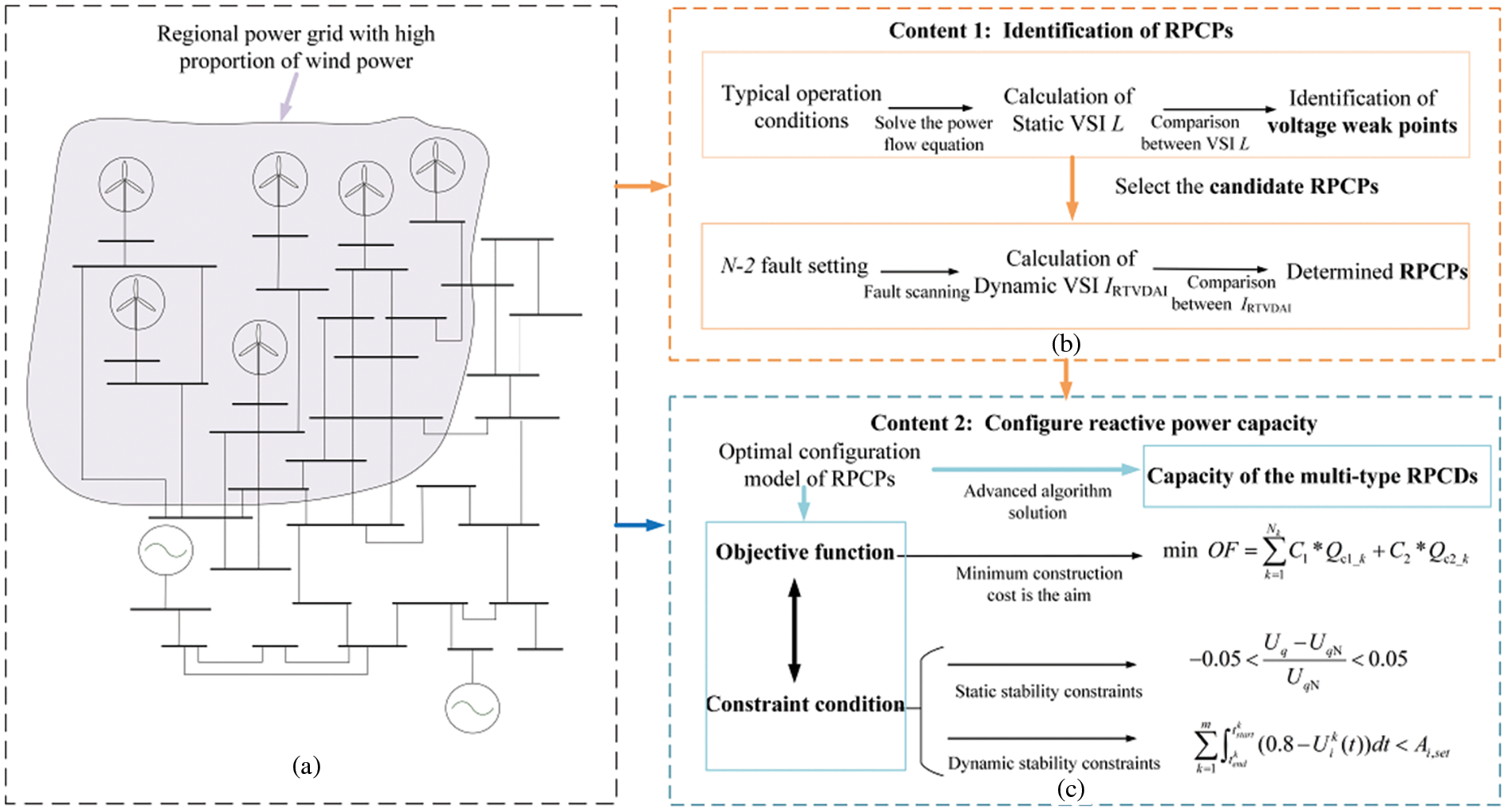
Figure 1: Schematic diagram of the overall strategy framework
The proposed method outlined in this paper entails a systematic approach to optimizing the allocation of RPCDs within transmission grids. Comprising two fundamental stages, this method begins with the meticulous selection of allocation points for RPCDs, followed by the allocation of capacities for the chosen devices. These steps, crucial for enhancing grid stability and efficiency, are clearly delineated in Fig. 1b,c, providing a visual roadmap of the entire process.
To initiate the allocation process, weak voltage points within the grid are identified as potential candidate points based on the proposed static VSI under typical scenarios. Subsequently, a comprehensive evaluation is conducted through N-2 fault scanning on the lines connected to these weak voltage points, assessing their dynamic VSI. By integrating both static and dynamic considerations, the final reactive power compensation points (RPCPs) are determined. This meticulous selection process ensures the robust placement of RPCDs capable of effectively addressing voltage stability concerns across various operational scenarios.
Moving on to the capacity allocation stage, a multi-type reactive power compensation device optimization model is developed for the RPCPs. This model, designed to minimize construction costs while adhering to constraints related to both static and dynamic voltage stability, forms the crux of the capacity allocation process. Leveraging advanced optimization algorithms, the model facilitates the determination of optimal capacities for static and dynamic RPCDs. This ensures static voltage stability under typical operating conditions while providing substantial dynamic reactive power support during transient processes, thus enhancing the overall resilience of the transmission grid. Through the systematic implementation of these steps, the proposed method aims to pave the way for efficient and cost-effective integration of reactive power compensation devices, fostering a more sustainable and reliable energy infrastructure.
3 Voltage Operation Characteristics of Regional Power Grid with High Proportion of WP
Based on the operating principles of wind turbines, this chapter analyzes the influence mechanisms of grid-connected WP system on grid voltage. Additionally, considering the common RPCDs in regional power grids with high proportion of WP, the operational characteristics are elucidated through the mathematical models constructed for typical static and dynamic RPCDs.
3.1 Influence on Voltage Stability of Regional Power Grid for Intensive Access of WFs
Fig. 2 is a schematic diagram of the grid-connected WP system. In this figure,
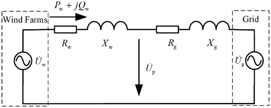
Figure 2: Schematic diagram of grid connection equivalent of WF
Taking the system equivalent voltage vector
where Pw and Qw represent the active power and reactive power output of the wind turbine, respectively.
Assuming the system is an infinite source, denoted by
In the voltage drop equation, the voltage amplitude difference is mainly determined by the longitudinal component of the voltage drop, while the phase angle difference of the voltage is determined by the transverse component. During WF operation, it is required to supply reactive power to the power grid in order to maintain a constant power factor. Therefore, according to Eq. (1), when the active power output Pw and reactive power output Qw of the wind turbine change, the amplitude of the wind turbine terminal voltage
As the proportion of WP in the system continues to increase, the fluctuation characteristics of WP output will not only affect the voltage at the junction point, but also have a great impact on the voltage of each node in the grid system connected to the WF. Therefore, it is no longer applicable to use infinite power supply for equivalent value in the grid-connected system. If the infinite power grid in Fig. 2 evolves into a regular node with load, that is,
3.2 Operation Characteristics of RPCDs
Due to the discrete nature of static RPCD during actual operation, preset switching commands are established during grid dispatch, hence their operational status typically affects the system’s static voltage stability criteria. In contrast, dynamic RPCDs can output continuous reactive power based on predetermined reference voltage values during transient processes, thereby enhancing the system’s dynamic voltage stability criteria. This section analyzes the operational characteristics of different types of reactive power compensation devices through the mathematical models of two typical devices.
Capacitor Bank (CB) and Static Synchronous Compensator (STATCOM) are selected as typical static RPCDs and dynamic RPCDs in this section, respectively. The working principles of each device are analyzed separately.
The operation principle of CBs for reactive power compensation is based on their connection or disconnection to regulate the reactive power of system. When the CB is connected to the system, it can provide reactive power compensation; When it is disconnected, it does not provide reactive power compensation. The expression for the reactive power output QCB of the CB is given by:
where CCB is the total capacitance of the CB; UCB is the voltage at both terminals of the CB; ω is the angular frequency of the grid.
CB, as the most widely used RPCD, has the advantages of wide adjustment range, low investment cost and high technical maturity. However, their discrete operational characteristics limit their flexibility and responsiveness in meeting the precise and rapid dynamic adjustment requirements of modern power systems during real-time operations.
STATCOM is a bridge converter made up of fully controllable power electronic components designed for dynamic RPCD applications. Leveraging power electronic devices, STATCOM demonstrates exceptionally rapid dynamic response capabilities, capable of addressing the system’s reactive power demands within milliseconds. It enables precise control over both the magnitude and phase angle of the output voltage, allowing for accurate reactive power compensation in line with predefined reference values. The mathematical expression for the reactive power output of STATCOM is given by:
where QSTAT is the reactive power provided or absorbed by STATCOM; USTAT is the output voltage amplitude of STATCOM; ISTAT is the output current amplitude of STATCOM; δSTAT is the phase angle of the output voltage; θg is the phase angle of the grid voltage.
When the loss is ignored, the operational schematic diagram is shown in Fig. 2. Where
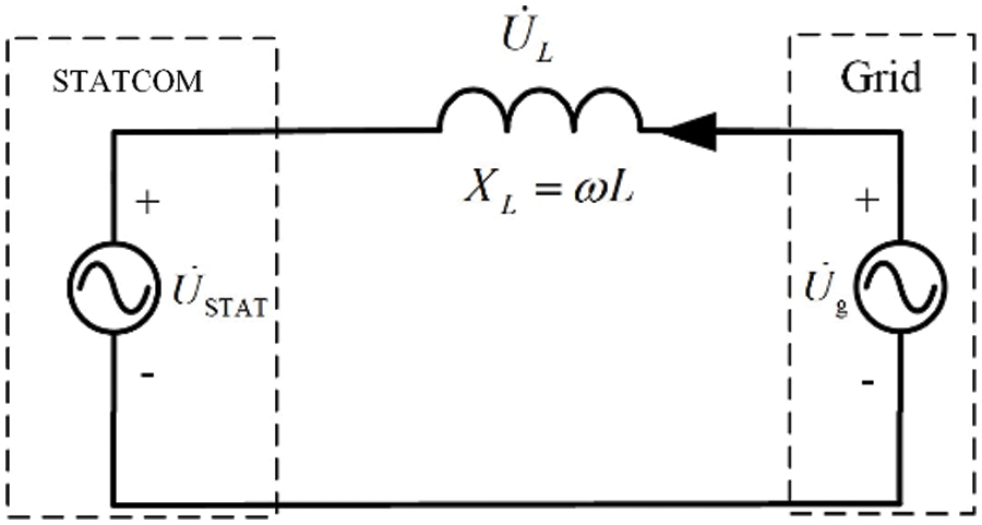
Figure 3: STATCOM grid-connected equivalent diagram
When
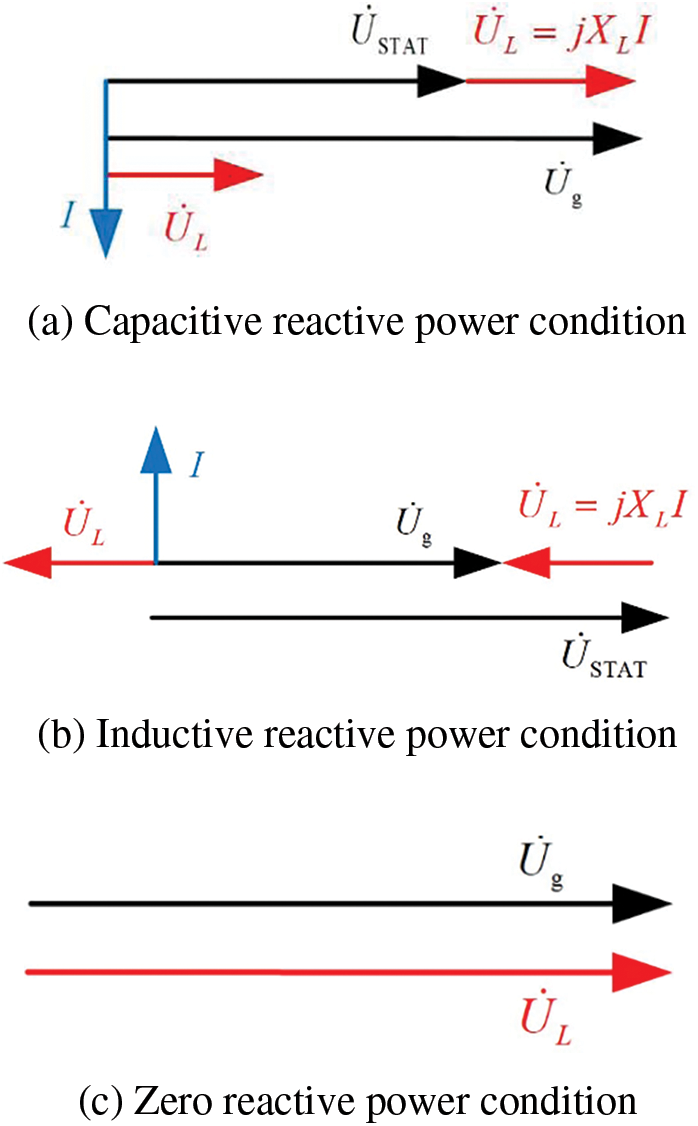
Figure 4: Phasor diagram of STATCOM grid-connected operation
When
When
Static VSI and dynamic VSI are proposed to identify RPCPs in this chapter. The specific logic is: static VSI of all nodes in the regional power grid can be calculated under the selected typical operation conditions, and the range of candidate points of RPCPs can be defined. Further, in order to analyze the voltage dynamic operation capability of the candidate points of the RPCPs, an N-2 fault scan is performed on the outgoing line of the target to be selected point, and the dynamic VSI of the target to be selected point is calculated to determine the configuration point of the reactive power compensation device. Its logical structure is shown in the Fig. 5.
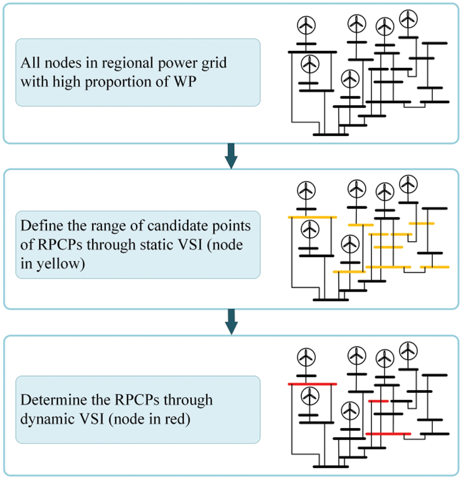
Figure 5: Diagram of the relationship between static VSI and dynamic VSI
In this paper, Lj is adopted as the static VSI under typical operation condition with high output of WF, which depends on the power flow calculation results under typical operation conditions. Therefore, the node admittance matrix of the system needs to be read and constructed to form the corresponding equation of state:
where IG and UG are the current vector and voltage vector of the injected power supply node, respectively; IL and UL are the current vector and voltage vector of the send-out nodes, respectively; YLL and YGG are self-admittance between the send-out nodes and injection power nodes, and YLG and YGL are mutual admittance between the send-out nodes and injection power nodes.
Solve the power flow equation under typical operation condition with high output of WF, and calculate the power flow distribution of each substation according to the power flow solution results. The equivalent output power expression of substation j is as follows:
where a is the send-out node connected to the j-th substation; A is the total number of send-out nodes connected to the j-th substation; Pa + jQa is the power of the a-th send-out node.
The static VSI L of each substation of the WF grid-connected system is calculated by calculating the result of the power flow equation under typical operating conditions. Taking substation j as an example, the calculation expression of the static VSI Lj is as follows:
where Ui is the bus voltage vector of the i-th substation;
Based on the calculated VSI L of each substation, the average value Lave of static VSI L of all substations is obtained, and the static VSI L of each substation is compared with the average value Lave. If the static VSI L of the substation is greater than the average value Lave, i.e., Lj > Lave, it can be judged that the substation is the weak point of static voltage stability. The set mL of weak point of static voltage stability is used as the reactive power compensation candidate point.
The dynamic VSI is based on the area of dynamic voltage drop and is designed to compare the voltage support capabilities of various nodes during major disturbances, and it quantifies the extent to which voltage weak nodes affect other nodes. This paper takes N-2 fault as a typical large disturbance fault, and the schematic diagram of the N-2 fault disturbance of the line is shown in Fig. 6.
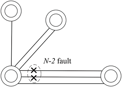
Figure 6: Schematic diagram of the N-2 fault disturbance of the line
Take voltage weak node j as an example, if there are M adjacent nodes of this node, and the node has a total of QN outgoing lines, scanning all the set N-2 faults, and calculating the dynamic voltage drop area SRTVDAI,j,t of each adjacent node under each large disturbance condition, and the expression for the relative dynamic VSI IRTVDAI,j can be obtained:
where
where SRTVDAI,j(f) is the dynamic voltage drop area of all adjacent nodes of the j-th static voltage stability weak point under fault f, M is the number of adjacent nodes of the static voltage stability weak point j, F is the number of check faults of the j-th static voltage stability weak point, IRTVDAI,j is the maximum value of SRTVDAI,j(f) under each check fault is taken.
When a certain N-2 fault occurs, the dynamic voltage drop area SRTVDAI,j,t of the i-th adjacent node is calculated as follows:
where SRTVDAI,i is the dynamic voltage drop area of the i-th adjacent node under each N-2 fault disturbance condition, t’start is the moment when the i-th adjacent node first experiences voltage drop to 80% of its rated value, t’end is the moment when the voltage of the i-th adjacent node drops below or equal to 80% of its rated value and then recovers and remains above 80% of its rated value, Ui_N is the voltage rated value of the i-th adjacent node, and ui(t) is the voltage trajectory curve of the i-th node under the fault.
Based on the calculation method described above, the relative dynamic VSI IRTVDAI,j is obtained for each reactive power compensation candidate point in the set mL of static voltage weak nodes. This index is then sorted in descending order to form the set mI, and finally the final RPCP can be determined based on actual planning demand.
5 Optimal Configuration Model of RPCD
The RPCP can be determined according to the static VSI and the dynamic VSI, and then the specific installed capacity of the static RPCD and the dynamic RPCD at each RPCP need to be determined, respectively. This chapter designs the optimal configuration model for the RPCDs that considers both static and dynamic voltage stability conditions.
As the construction cost of RPCDs is high, the proposed model aims to minimize the total construction cost of the RPCDs at each compensation point. The objective function is equated as follows:
where C1 is the unit capacity construction cost of static RPCD; C2 is the unit capacity construction cost of the dynamic RPCD; Qc1_k is the capacity of static RPCD at the k-th point of reactive power compensation; Qc2_k is the capacity of the dynamic RPCD at the k-th point of reactive power compensation; Nk is the total number of RPCPs.
Static stability constraints consist of power flow constraint, node voltage constraint, RPCD capacity constraint under typical operation conditions, and dynamic stability constraints consist of dynamic voltage stability constraints under N-2 fault scanning.
5.2.1 Static Stability Constraints
Under static stability constraint, the capacity Q’c1_k of the static RPCD and the capacity Q’c2_k of the dynamic RPCD, as decision variables, need to satisfy the power flow constraint, node voltage constraint and capacity constraint of the RPCD under typical operation conditions. Among them, the power flow constraint under typical operation conditions of the high output of WF is:
The power expression of the node under typical operation conditions of the high output of WF is as follows:
where the power expression of RPCP k is:
where Φ(p,:) and Φ(:,p) are the branch sets where node p is at the beginning and ending ends, respectively; q is the power injection node; t is the power output node; ψ is the set of system AC nodes; Uq is the voltage of the q-th node; Pqp is the active power on the branch qp; Qqp is the reactive power on the branch qp; Rqp is the equivalent resistance of the branch qp; Xqp is the equivalent reactance of the branch qp; Pp is the active power injected by the p-th node; Qp is the reactive power injected by node p; Pw_max is the output data of WF under typical operation conditions of the high output of WF; θw is the power factor of WF; Pk is the active power injected by the k-th RPCP; Qk is the original reactive power injected at the k-th RPCP; Q’c1_k is the capacity of static RPCD configured at the k-th RPCP;
where the power expression of each node is:
where Pp1 is the active power output of the p-th node, Pp2 is the active power load of the p-th node, Qp1 is the reactive power output of the p-th node, and Qp2 is the reactive power load of the p-th node.
The reactive power expression of the k-th RPCP:
where Qk is the original reactive power injected by the k-th node for reactive power compensation configuration.
According to the safe operation requirements of the power grid [35], and the system node voltage constraint expression is as follows:
where UqN is the operation voltage rating of the q-th node, and Uq is the operation voltage value of the q-th node.
The capacity constraint expression of the RPCD is:
where Qc1_k_min and Qc1_k_max are the lower limit and upper limit of the configured capacity of the static RPCD at the k-th RPCP; Qc2_k_min and Qc2_k_min are the lower limit and upper limit of the configured capacity of the dynamic reactive power compensation equipment at the k-th RPCP; Qc1_k is the capacity of static RPCD configured at the k-th RPCP; Qc2_k is the capacity of the dynamic RPCD configured at the k-th RPCP.
5.2.2 Dynamic Stability Constraints
Under the dynamic voltage stability constraints, the dynamic reactive power support capacity Qc2_k in the dynamic RPCD, as a decision variable, needs to satisfy the dynamic voltage stability constraints. The specific implementation method involves scanning the N-2 faults in the outgoing lines of the reactive power compensation nodes, combined with its corresponding dynamic voltage drop area SRTVDAI,j,t, and establish the dynamic voltage stability constraint under large disturbance:
where Ai,set is the threshold value of the critical transient voltage drop area of the i-th node, tkstart is the moment when voltage drops to 0.8 p.u. for the k-th time of a fault, tkend is the moment when the voltage recovers to above 0.8 p.u. for the k-th time of a fault; Uki(t) is the voltage trajectory curve of the i-th node for the k-th time of a fault when the voltage drops below 0.8 p.u.; m is the total number of curves with voltage below 0.8 p.u. under a certain fault.
The specific calculation method of Ai,set is to conduct multi-type fault simulation on the i-th node in advance, and select the critical value of the maximum voltage drop area under the condition of voltage stability. The equation is as follows, where Aj,i,set is the integral value of the voltage drop area under the j-th type of fault:
5.3 Model Solving Based on PSO Algorithm
The optimal configuration model of RPCD built in Sections 5.1 and 5.2 is a typical optimization model with multiple decision variables and multiple constraints. Therefore, particle swarm optimization (PSO) algorithm is used in this section to solve the capacity of static RPCD and dynamic RPCD configured by RPCP.
The fundamental concept of the PSO algorithm is as follows: Firstly, determining the number of particles N and initializing their positions and velocities, while setting objective function. Secondly, establishing upper and lower limits for the positions and velocities of each particle. Next, computing the fitness of each particle. Subsequently, comparing the fitness of the current particle with its own historical best solution and the global best solution, updating both accordingly. Then, iterating to update the velocities and positions of particles according to the iteration formula. If the set target condition is not met, the process returns to the previous step, and the condition of ending the optimization process is generally to meet the convergence condition required by the model or to reach the set number of iterations.
The expression for updating the position and velocity of the particle based on the two related extreme values of the historical optimal solution and the global optimal solution is as follows:
where
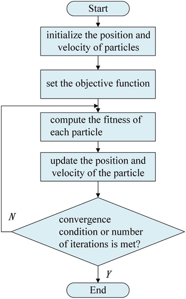
Figure 7: Flow chart of PSO algorithm
To apply the PSO algorithm to solve the capacity optimization model of RPCD constructed in this paper, the number of particle swarm initialization should be determined according to the number of RPCP, and the reactive power capacity of static RPCD and dynamic RPCD to be obtained should be taken as the optimization target, that is, the particle position in the PSO algorithm. In the optimization process, each decision variable in the iterated particle position set is put into the static stability constraint and the dynamic stability constraint to judge. If all constraints are met, the construction cost of RPCD under the decision variable is calculated by Eq. (11), and the process is iterated repeatedly until the target construction cost is met. In this case, the value of the decision variable is the reactive power capacity configured by RPCD.
To validate the effectiveness of the proposed method in this paper, the modified 68 bus system is used as the research subject, and topological diagram is shown in Fig. 8. A corresponding system model is built in the PST toolbox of simulation software MATLAB. The system model consists of 68 nodes, including 16 generator nodes and 52 load nodes.
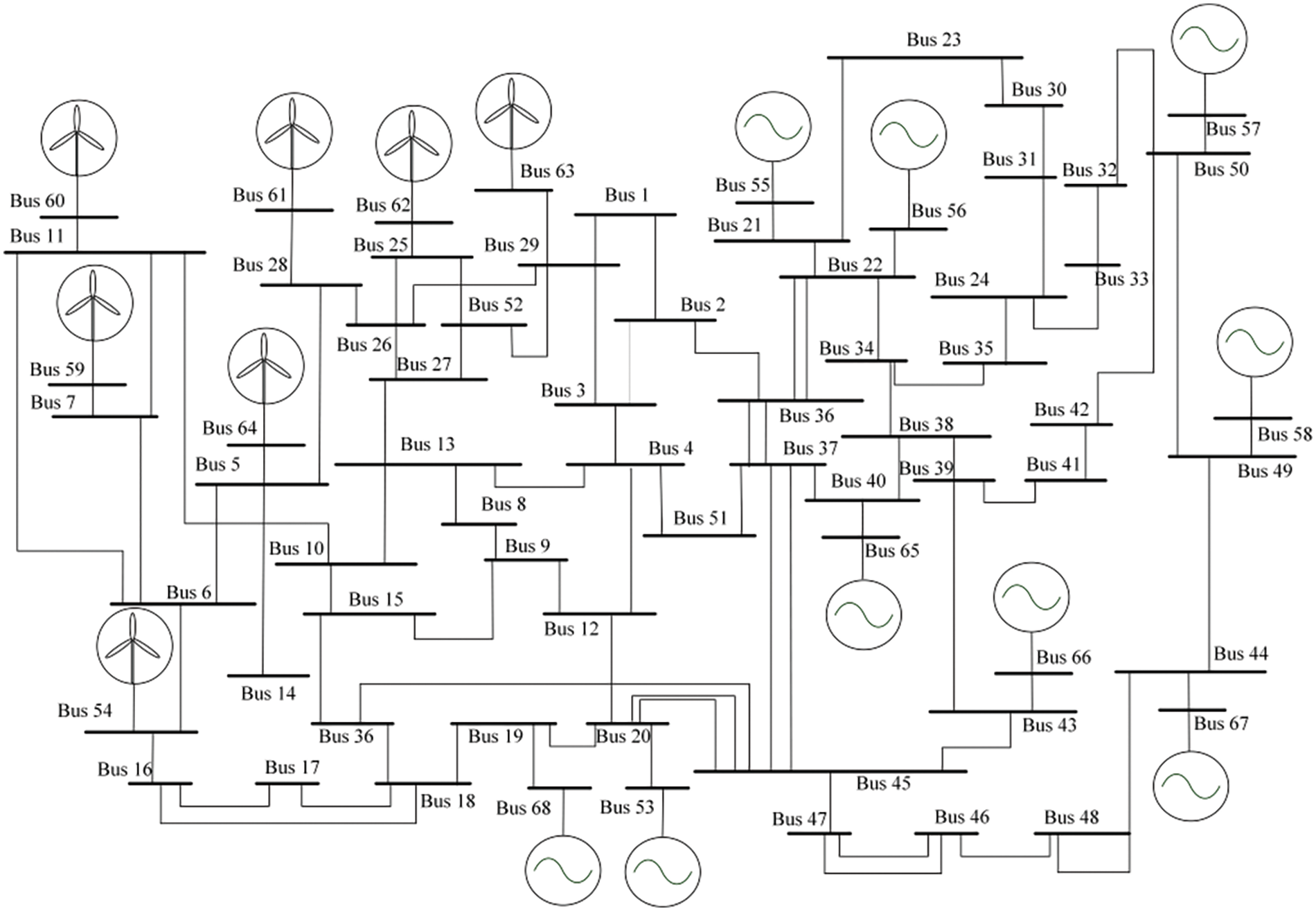
Figure 8: Topological diagram of modified 68 bus system
6.1 Identification of Reactive Power Compensation Configuration Points
6.1.1 Selection of Static Voltage Weak Nodes
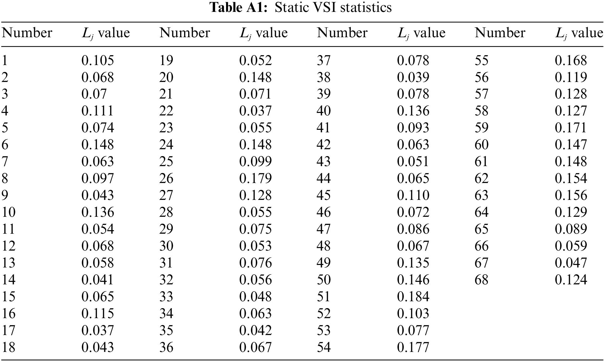
According to Eqs. (5) to (7) in Section 3.1, the static VSI Lj of each node in the system is calculated, and the calculation results are shown in Fig. 9. Calculate the average value L of static VSI Lave, and compare the static VSI Lj of each node with Lave. Nodes 6, 10, 20, 24, 26, 36, 37, 39, 40, 41, 42, 44, 45, 49, 50, 51, 52, 54, 59, 60, 61, 62, 63 are identified as static voltage weak nodes, which serve as the reactive power compensation candidate point. Specific values are given in the Table A1.
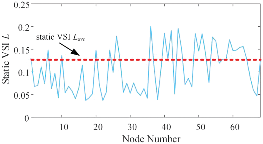
Figure 9: Statistical diagram of static VSI statistics
6.1.2 Calculation of Dynamic Voltage Drop Area of Voltage Weak Nodes
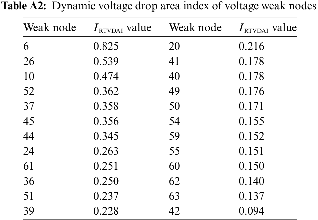
Perform N-2 fault scan for voltage weak nodes, and the system experiences a fault at 3.0 s. Based on Eqs. (8) and (10), calculate the dynamic voltage drop area index IRTVDAI of voltage weak nodes. The calculation results of the dynamic voltage drop area index IRTVDAI for voltage weak nodes, sorted in descending order, are summarized in Fig. 10. Specific values are given in the Table A2.
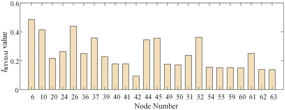
Figure 10: Statistical diagram of IRTVDAI value of voltage weak nodes
Based on the descending order of the dynamic voltage drop area index IRTVDAI, it is observed that the 6-th, 26-th and 10-th node have relatively high values. Therefore, these nodes from the set of voltage weak nodes are selected as for RPCPs. Performing an N-2 fault scan for the lines connected to the RPCPs, and the following uses the 6-th node as an example, the voltage dynamic operation curves of adjacent nodes for the RPCP are shown in Fig. 11.
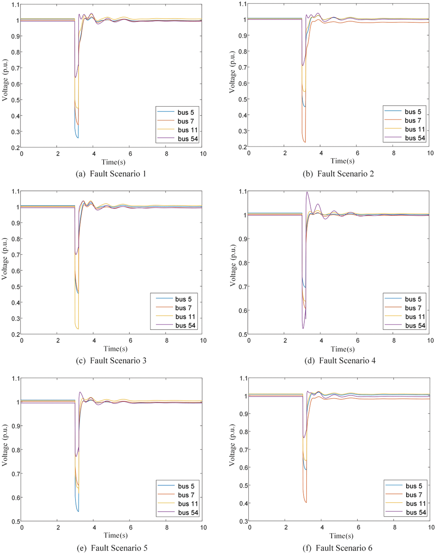
Figure 11: Voltage dynamic operation curve of adjacent nodes of the 6-th node
It can be seen from the index calculation method mentioned in Section 4.2 and the dynamic operation curves of each weak node that the voltage stability weak node with more adjacent nodes has a larger dynamic voltage drop area index IRTVDAI,j, which can be used as the selected point for reactive power compensation.
6.2 Reactive Capacity Optimization of RPCDs
Using the reactive power optimal configuration model proposed in Sections 3.1 and 3.2, which considers both static and dynamic voltage stability, the capacities of the RPCDs are optimized for the selected RPCPs. The unit construction cost C1 of the static RPCD is set at 8600 $/MVar, and the unit construction cost C2 of the dynamic RPCD is set at 24,800 $/MVar.
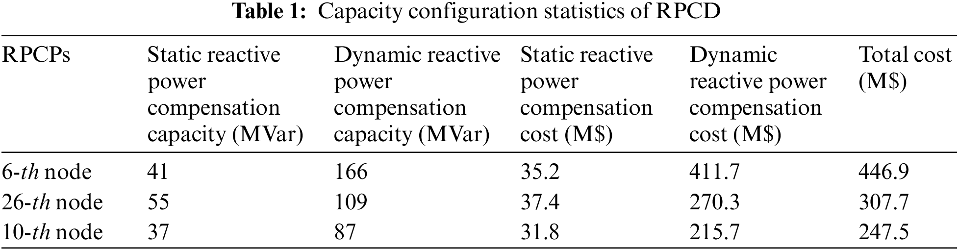
In Section 5.3, it is proposed to solve the capacity optimization model of RPCD constructed by using PSO algorithm. Since three RPCPs are determined in Section 6.1, the particle swarm number N can be set to 15. At the same time, according to the capacity results of RPCD configured by bus nodes in the actual project, and let the initial capacity of the static RPCD and dynamic RPCD configured for the three nodes be 40 and 100 MVar. After optimization and solution by PSO algorithm, the capacity of static RPCD configured at the 6-th node, 26-th and 10-th node is 41 MVar, 55 MVar and 37 MVar, and the capacity of dynamic RPCD is 166, 109 and 87 MVar. The relevant statistics are provided in Table 1.
According to the solution results of the proposed optimization model, the capacity of the static RPCD configured at each RPCP is obtained. The power flow equations are solved for the same typical scenario, and based on the power flow results, it is found that during steady-state operation, the voltage at the 6-th node increases from 0.946 to 1.009 p.u., the voltage at the 10-th node increases from 0.937 to 1.018 p.u., and the voltage at the 26-th node increases from 0.939 to 1.026 p.u. after the optimization configuration. The voltage performance of every node has seen significant enhancements, with a comparison of the static voltage operation shown in Fig. 12. It should be noted that high nodes are nodes of power supply or nodes that are far away from the regional power grid in the dense access areas of new energy stations, so under typical working conditions, the voltage change of high nodes is small.
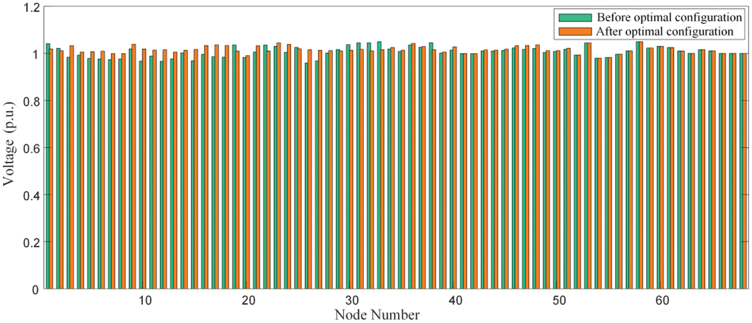
Figure 12: Comparison of static voltage operation of each node
In addition, in order to highlight the voltage operation problem faced by the research object in the calculation example, in this example, RPCDs are assumed to be configured at the grid-connected point of WF to ensure voltage stability. As can be seen from the figure, the 40-th to 68-th node are the grid-connected points of the power source or nodes far away from the regional power grid with a high proportion of WP. Therefore, under typical working conditions, the voltage variation of these nodes is small.
Taking the most common single-phase short circuit fault in practical operation as a typical fault, single-phase short circuit faults with a grounding resistance of 0.1Ω is set at the RPCP to analyze the voltage dynamic characteristics of each node and adjacent nodes before and after the optimization configuration of RPCDs. The following uses the 6-th node as an example, Fig. 13 below respectively shows the voltage operation curves of the 6-th node during the occurrence of typical faults.
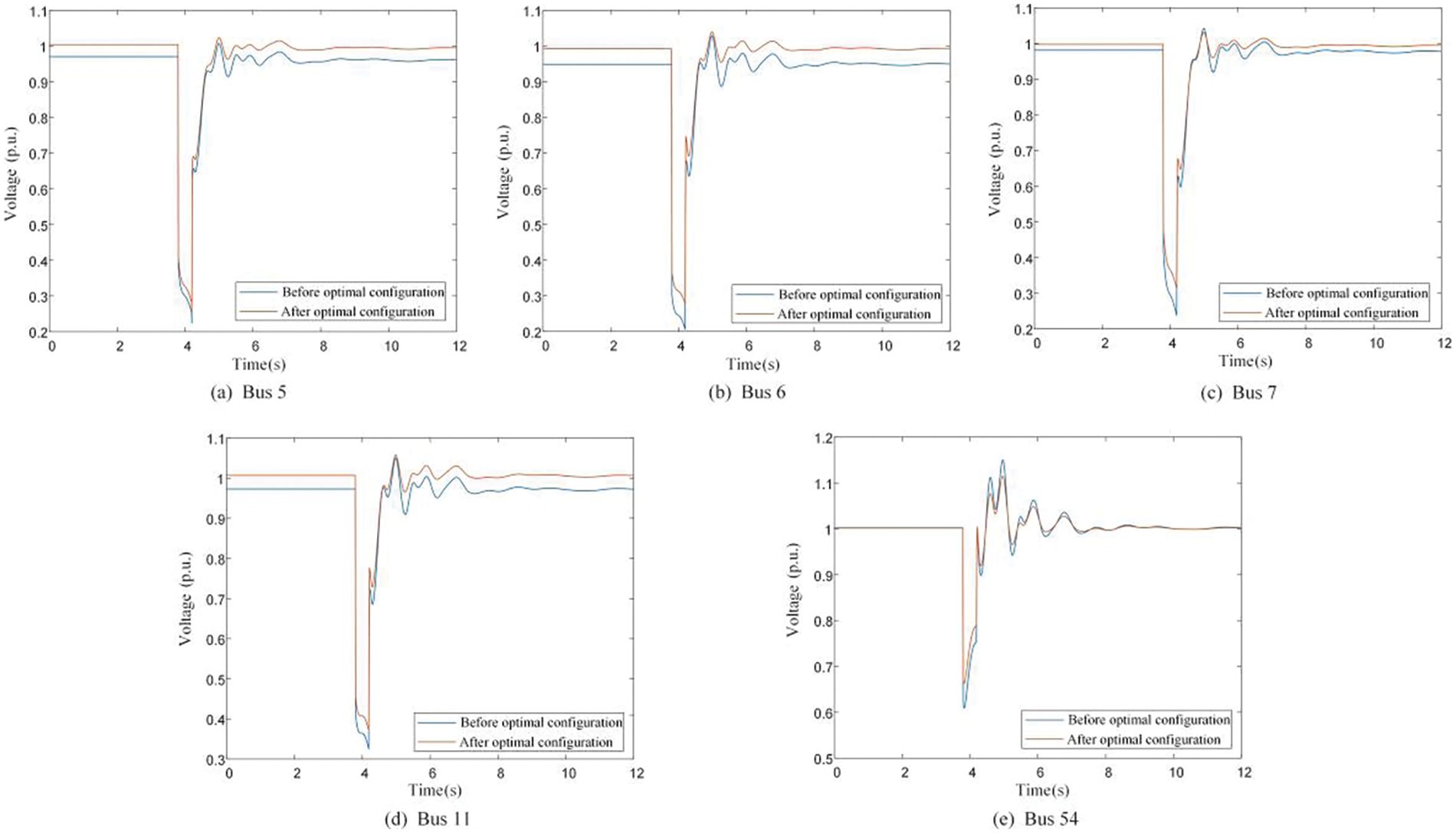
Figure 13: Dynamic operation curves of relevant nodes of the 6-th node under typical fault
It can be observed that configuration of RPCDs at the voltage weak nodes significantly improves the voltage dynamic characteristics of the originally weak nodes. The lowest voltage drop point is elevated, and the operation voltage is restored to 0.8 p.u. in a shorter time. Additionally, the dynamic characteristics of the adjacent nodes of the configured RPCD nodes are also improved.
This paper presents an optimal configuration method for multi-type RPCDs in regional power grids with a high proportion of wind power. The proposed method systematically identifies the location and determines the capacity of the required RPCDs for a regional power grid model that facilitates intensive access to WFs. It enhances the operational capacity of voltage-weak nodes in the system and ensures static and dynamic voltage stability in regional power grids with a high proportion of WP. Moreover, this method exhibits high economic efficiency, and it is deemed as a crucial support for achieving large-scale grid-connected WFs.
It is important to note that the proposed method for identifying voltage weak nodes based on VSI considers a limited range of typical operational conditions. Additionally, the optimization configuration model for RPCDs solely considers construction costs without factoring in the operational costs of RPCDs and the regulation capabilities of different types of RPCDs. Addressing these deficiencies will be the primary focus of future research.
Acknowledgement: We would like to thank all those who have reviewed and contributed to this paper for their valuable assistance.
Funding Statement: This work was supported by the Science and Technology Project of State Grid Corporation Headquarters (No. 5100-202323008A-1-1-ZN).
Author Contributions: The authors confirm contribution to the paper as follows: study conception and design: Ying Wang, Cangbi Ding; data collection: Jie Dang, Chenyi Zheng; analysis and interpretation of results: Ying Wang, Yi Tang; draft manuscript preparation: Ying Wang, Cangbi Ding. All authors reviewed the results and approved the final version of the manuscript.
Availability of Data and Materials: Not applicable.
Ethics Approval: Not applicable.
Conflicts of Interest: The authors declare that they have no conflicts of interest to report regarding the present study.
References
1. A. Z. A. Shaqsi, K. Sopian, and A. Al-Hinai, “Review of energy storage services, applications, limitations, and benefits,” Energy Rep., vol. 6, no. 5, pp. 288–306, Dec. 2020. doi: 10.1016/j.egyr.2020.07.028. [Google Scholar] [CrossRef]
2. Y. Hao, D. Su, and Z. Lei, “Optimal intelligence planning of wind power plants and power system storage devices in power station unit commitment based,” Energy Eng., vol. 119, no. 5, pp. 2081–2104, Jul. 2022. doi: 10.32604/ee.2022.021342. [Google Scholar] [CrossRef]
3. L. Wang, Z. Wang, Y. Yang, S. Zhou, Y. Dong and F. Zhang, “Review on wind power development and relevant policies between China and Japan,” Energy Eng., vol. 118, no. 6, pp. 1611–1626, Sep. 2021. doi: 10.32604/EE.2021.016010. [Google Scholar] [CrossRef]
4. X. Zhou, C. Ding, J. Dai, Z. Li, Y. Hu and Z. Qie “An active power coordination control strategy for AC/DC transmission systems to mitigate subsequent commutation failures in HVDC systems” Electronics, vol. 10, no. 23, pp. 3044, Dec. 2021. doi: 10.3390/electronics10233044. [Google Scholar] [CrossRef]
5. S. Sun, P. Yu, J. Xing, Y. Cheng, S. Yang and Q. Ai, “Short-term wind power prediction based on ICEEMDAN-SE-LSTM neural network model with classifying seasonal,” Energy Eng., vol. 120, no. 12, pp. 2761–2782, Nov. 2023. doi: 10.32604/ee.2023.042635. [Google Scholar] [CrossRef]
6. I. D. Margaris, S. A. Papathanassiou, N. D. Hatziargyriou, A. D. Hansen, and P. Sorensen, “Frequency control in autonomous power systems with high wind power penetration,” IEEE Trans. Sustain. Energy, vol. 3, no. 2, pp. 189–199, Apr. 2012. doi: 10.1109/TSTE.2011.2174660. [Google Scholar] [CrossRef]
7. L. Xiang, H. Zhu, Y. Zhang, Q. Yao, and A. Hu, “Impact of wind power penetration on wind-thermal-bundled transmission system,” IEEE Trans. Power Electron., vol. 37, no. 12, pp. 15616–15625, Dec. 2022. doi: 10.1109/TPEL.2022.3189366. [Google Scholar] [CrossRef]
8. M. Bakhtvar and A. Keane, “Allocation of wind capacity subject to long term voltage stability constraints,” IEEE Trans. Power Syst., vol. 31, no. 3, pp. 2404–2414, May 2016. doi: 10.1109/TPWRS.2015.2454852. [Google Scholar] [CrossRef]
9. S. Nikkhah and A. Rabiee, “Optimal wind power generation investment, considering voltage stability of power systems,” Renew. Energy, vol. 115, pp. 308–325, Jan. 2018. doi: 10.1016/j.renene.2017.08.056. [Google Scholar] [CrossRef]
10. W. Bao, L. Ding, Z. Liu, G. Zhu, M. Kheshti and Q. Wu, “Analytically derived fixed termination time for stepwise inertial control of wind turbines—Part I: Analytical derivation,” Int. J. Electr. Power Energy Syst., vol. 121, pp. 1–10, Oct. 2020. [Google Scholar]
11. F. Xiao et al., “The short-term prediction of wind power based on the convolutional graph attention deep neural network,” Energy Eng., vol. 121, no. 2, pp. 359–376, Jan. 2024. doi: 10.32604/ee.2023.040887. [Google Scholar] [CrossRef]
12. B. Chen, F. Miao, J. Yang, C. Qi, and W. Ji, “A temporary frequency response strategy using a voltage source-based permanent magnet synchronous generator and energy storage systems,” Energy Eng., vol. 121, no. 2, pp. 541–555, Jan. 2024. doi: 10.32604/ee.2023.028327. [Google Scholar] [CrossRef]
13. H. Zhang, C. Li, Q. Wei, and Y. Zhang, “Fault detection and diagnosis of the air handling unit via combining the feature sparse representation based dynamic SFA and the LSTM network,” Energy Build., vol. 269, no. 4, pp. 112241, Aug. 2022. doi: 10.1016/j.enbuild.2022.112241. [Google Scholar] [CrossRef]
14. T. F. Megahed, E. F. Morgan, P. N. Timo, and M. Saeed, “Neural network predictive control for fault detection and identification in DFIG with SMES for low voltage ride-through requirements,” Ain Shams Eng. J., vol. 15, no. 7, pp. 102775, Apr. 2024. doi: 10.1016/j.asej.2024.102775. [Google Scholar] [CrossRef]
15. X. Ge, J. Qian, Y. Fu, W. J. Lee, and Y. Mi, “Transient stability evaluation criterion of multi-wind farms integrated power system,” IEEE Trans. Power Syst., vol. 37, no. 4, pp. 3137–3140, July 2022. doi: 10.1109/TPWRS.2022.3156430. [Google Scholar] [CrossRef]
16. H. Zhang, W. Yang, W. Yi, J. B. Lim, Z. An and C. Li, “Imbalanced data based fault diagnosis of the chiller via integrating a new resampling technique with an improved ensemble extreme learning machine,” J. Build. Eng., vol. 70, no. 2, pp. 106338, July 2023. doi: 10.1016/j.jobe.2023.106338. [Google Scholar] [CrossRef]
17. A. Boričić, J. L. R. Torres, and M. Popov, “Fundamental study on the influence of dynamic load and distributed energy resources on power system short-term voltage stability,” Int. J. Electr. Power Energy Syst., vol. 131, no. 2, pp. 107141, Oct. 2021. doi: 10.1016/j.ijepes.2021.107141. [Google Scholar] [CrossRef]
18. S. Munikoti, B. Natarajan, K. Jhala, and K. Lai, “Probabilistic voltage sensitivity analysis to quantify impact of high PV penetration on unbalanced distribution system,” IEEE Trans. Power Syst., vol. 36, no. 4, pp. 3080–3092, Jul. 2021. doi: 10.1109/TPWRS.2021.3053461. [Google Scholar] [CrossRef]
19. B. Ismail, N. I. Abdul Wahab, M. L. Othman, M. A. M. Radzi, K. Naidu Vijyakumar and M. N. Mat Naain, “A comprehensive review on optimal location and sizing of reactive power compensation using hybrid-based approaches for power loss reduction, voltage stability improvement, voltage profile enhancement and loadability enhancement,” IEEE Access, vol. 8, pp. 222733–222765, 2020. doi: 10.1109/ACCESS.2020.3043297. [Google Scholar] [CrossRef]
20. E. Vittal, M. O’Malley, and A. Keane, “A steady-state voltage stability analysis of power systems with high penetrations of wind,” IEEE Trans. Power Syst., vol. 25, no. 1, pp. 433–442, Feb. 2010. doi: 10.1109/TPWRS.2009.2031491. [Google Scholar] [CrossRef]
21. B. B. Adetokun, C. M. Muriithi, and J. O. Ojo, “Voltage stability assessment and enhancement of power grid with increasing wind energy penetration,” Int. J. Electr. Power Energy Syst., vol. 120, no. 2, pp. 105988, Sep. 2020. doi: 10.1016/j.ijepes.2020.105988. [Google Scholar] [CrossRef]
22. J. Then, A. P. Agalgaonkar, and K. M. Muttaqi, “Hosting capacity of an australian low-voltage distribution network for electric vehicle adoption,” IEEE Trans. Ind. Appl., vol. 60, no. 2, pp. 2601–2610, Mar.–Apr. 2024. doi: 10.1109/TIA.2023.3337068. [Google Scholar] [CrossRef]
23. H. Zaheb et al., “A contemporary novel classification of voltage stability indices,” Appl. Sci., vol. 10, no. 5, pp. 1639, Feb. 2020. doi: 10.3390/app10051639. [Google Scholar] [CrossRef]
24. Y. Li, Q. Chen, L. Wu, Y. Yan, and J. Zhou, “Wind farm reactive power demand analysis based on sensitivity and stability constraints considering wind speed fluctuations,” IEEE Trans. Power Syst., vol. 36, no. 2, pp. 1465–1477, Sep. 2020. [Google Scholar]
25. S. Tamalouzt et al., “Enhanced direct reactive power control-based multi-level inverter for DFIG wind system under variable speeds,” Sustainability, vol. 13, no. 16, pp. 9060, Aug. 2020. doi: 10.3390/su13169060. [Google Scholar] [CrossRef]
26. J. Ouyang, T. Tang, J. Yao, and M. Li, “Active voltage control for DFIG-based wind farm integrated power system by coordinating active and reactive powers under wind speed variations,” IEEE Trans. Energy Convers., vol. 34, no. 3, pp. 1504–1511, Sep. 2019. doi: 10.1109/TEC.2019.2905673. [Google Scholar] [CrossRef]
27. Y. Guo, H. Gao, Q. Wu, H. Zhao, J. Østergaard, and M. Shahidehpour, “Enhanced voltage control of VSC-HVDC-connected offshore wind farms based on model predictive control,” IEEE Trans. Sustain. Energy, vol. 9, no. 1, pp. 474–487, Jan. 2018. doi: 10.1109/TSTE.2017.2743005. [Google Scholar] [CrossRef]
28. Y. Li, S. Zhang, Y. Li, J. Cao, and S. Jia, “PMU measurements-based short-term voltage stability assessment of power systems via deep transfer learning,” IEEE Trans. Instrum. Meas., vol. 72, pp. 1–11, Sep. 2023. doi: 10.1109/TIM.2023.3311065. [Google Scholar] [CrossRef]
29. T. Liu, X. Gu, S. Li, Y. Bai, T. Wang and X. Yang, “Static voltage stability margin prediction considering new energy uncertainty based on graph attention networks and long short-term memory networks,” IET Renew. Power Gener., vol. 17, no. 9, pp. 2290–2301, May 2023. doi: 10.1049/rpg2.12731. [Google Scholar] [CrossRef]
30. Y. Zhou, Z. Li, and G. Wang, “Study on leveraging wind farms’ robust reactive power range for uncertain power system reactive power optimization,” Appl. Energy, vol. 298, no. 4, pp. 117130, Sep. 2021. doi: 10.1016/j.apenergy.2021.117130. [Google Scholar] [CrossRef]
31. Y. Liu, D. Ćetenović, H. Li, E. Gryazina, and V. Terzija, “An optimized multi-objective reactive power dispatch strategy based on improved genetic algorithm for wind power integrated systems,” Int. J. Electr. Power Energy Syst., vol. 136, no. 4, pp. 107764, Mar. 2022. doi: 10.1016/j.ijepes.2021.107764. [Google Scholar] [CrossRef]
32. N. Gupta, “Probabilistic optimal reactive power planning with onshore and offshore wind generation, EV, and PV uncertainties,” IEEE Trans. Ind. Appl., vol. 56, no. 4, pp. 4200–4213, Jul.–Aug. 2020. [Google Scholar]
33. A. Radaideh, M. M. Bodoor, and A. Al-Quraan, “Active and reactive power control for wind turbines based DFIG using LQR controller with optimal gain-scheduling,” Electr. Comput. Eng., vol. 2021, no. 5, pp. 1–19, Oct. 2021. doi: 10.1155/2021/1218236. [Google Scholar] [CrossRef]
34. N. Wang, J. Li, W. Hu, B. Zhang, Q. Huang, and Z. Chen, “Optimal reactive power dispatch of a full-scale converter based wind farm considering loss minimization,” Renew. Energy, vol. 139, no. 2, pp. 292–301, 2019. doi: 10.1016/j.renene.2019.02.037. [Google Scholar] [CrossRef]
35. North American Electric Reliability Corporation, “Reliability guideline,” 2018. Accessed: Mar. 20, 2024. [Online]. Available: https://www.nerc.com/comm/RSTC_Reliability_Guidelines/Inverter-Based_Resource_Performance_Guideline.pdf [Google Scholar]
Appendix A
Cite This Article
 Copyright © 2024 The Author(s). Published by Tech Science Press.
This work is licensed under a Creative Commons Attribution 4.0 International License , which permits unrestricted use, distribution, and reproduction in any medium, provided the original work is properly cited.
 Downloads
 Citation Tools