
 Submit a Paper
 Propose a Special lssue
 Open Access
ARTICLE

A Cascading Fault Path Prediction Method for Integrated Energy Distribution Networks Based on the Improved OPA Model under Typhoon Disasters
1 Guangzhou Power Supply Bureau, Guangdong Power Grid Co., Ltd., CSG, Guangzhou, 510000, China
2 School of Electrical Engineering and Automation, Wuhan University, Wuhan, 430072, China
* Corresponding Author: Lei Chen. Email:
Energy Engineering 2024, 121(10), 2825-2849. https://doi.org/10.32604/ee.2024.052371
Received 31 March 2024; Accepted 31 May 2024; Issue published 11 September 2024
 View Full Text
 Download PDF
Abstract
In recent times, the impact of typhoon disasters on integrated energy active distribution networks (IEADNs) has received increasing attention, particularly, in terms of effective cascading fault path prediction and enhanced fault recovery performance. In this study, we propose a modified ORNL-PSerc-Alaska (OPA) model based on optimal power flow (OPF) calculation to forecast IEADN cascading fault paths. We first established the topology and operational model of the IEADNs, and the typical fault scenario was chosen according to the component fault probability and information entropy. The modified OPA model consisted of two layers: An upper-layer model to determine the cascading fault location and a lower-layer model to calculate the OPF by using Yalmip and CPLEX and provide the data to update the upper-layer model. The approach was validated via the modified IEEE 33-node distribution system and two real IEADNs. Simulation results showed that the fault trend forecasted by the novel OPA model corresponded well with the development and movement of the typhoon above the IEADN. The proposed model also increased the load recovery rate by >24% compared to the traditional OPA model.Keywords
Nomenclature
| CHP | Combined heat and power |
| DG | Distributed generator |
| ESS | Energy storage system |
| IEADN | Integrated energy active distribution network |
| OPF | Optimal power flow |
| PV | Photovoltaic |
| SOC | Self-organized criticality |
| α | Temperature factor |
| η | Energy transforming efficiency |
| θ | Angle between the wind and the line |
| λ | Heat transfer index of heat network pipes |
| μ | Constant inflecting the line type |
| π | Pressure matrix in the gas system |
| ω | Sub-objective function weights |
| A | Topological structure of different energy systems |
| B | Constant to reflect the temperature and efficiency of the compressor |
| Bij | Conductivity of branch ij |
| D | Line diameter |
| E | System information entropy |
| F | Power flow matrix |
| G | Solar radiation intensity |
| Gij | Conductors of branch ij |
| L | Load type |
| m | Number of energy coupling equipment |
| n | Quantity of energy coupling equipment |
| P | Combined component fault probability |
| Pfault | Component fault probability |
| Pflow | Operational failure probability |
| Pi | Active power injected into node i |
| PPV | Photovoltaic output power |
| p | Pressure applied to the lines and poles |
| p | Pressure matrix in the water system |
| Qi | Reactive power injected into node i |
| Rmax | Maximum typhoon velocity radius |
| r | Distance between the study location and the typhoon center |
| S | Source matrix |
| T | Temperature |
| Vi | Voltage amplitude of node i |
| v | Typhoon velocity |
| Z | Compression factor constant |
| zi,t | Fault situation on branch i at t |
In recent years, the frequency of extreme natural disasters, such as typhoons, has increased as global climate change intensifies [1]. The grid component failures will influence the security of the electricity grid caused by extreme natural disasters [2]. And the cascading fault from the initial component failures has great impact on the security of the power grid [3]. Situations of widespread electrical grid failures can significantly affect lives and the economy [4]. Integrated energy active distribution networks (IEADNs) have gradually become a research hotspot in the development of future energy networks owing to their multiple inter-coupled energy networks, as well as, extensive distributed generators (DGs) [5]. Since IEADNs serve as a crucial link for electrical power customers, their resilience under typhoons should be given adequate attention. Reducing damage due to extreme natural disasters is critical, and improving the safety and stability of IEADNs with favorable resilience is necessary [6].
IEADNs may have a relatively higher failure probability than power transmission networks due to more complex structures and weaker support capabilities [7]. Component fault probability and fault scenarios have been widely studied to discover methods for increasing IEADN resilience. These measures include early warning systems [8], pre-disaster reinforcement [9], emergency response [10], and post-disaster recovery [11]. As the resilience foundation improves, fast and accurate prediction of cascading IEADN fault development becomes highly critical.
Chen et al. [12] studied the dynamics of cascading failure iterating in a physical power distribution network, and defined node criticality based on electrical and structural characteristics to locate the network vulnerabilities. Liu et al. [13] analyzed the cascading failure risk of flexible interconnected distribution systems based on the physical structure of flexible multi-state switches and uncertain factors models. Bai et al. [14] modeled component damage due to extreme events and analyzed ADN fault repair schemes. Wang et al. [15] proposed an inverse-community structure to intuitively identify cascading fault risks and upgraded conventional modularity to quantify their characteristics in power networks. Gao et al. [16] developed a novel model to study cascading failure in cyber-physical power systems by considering the impact of voltage-related failures. Based on the interrelation analysis between the references [12–16], these methods are mainly based on the pure power distribution network and do not involve other form system so they cannot used in the IEADNs. In order to promote the methods into more complicated systems, the cascading fault path of the IEADNs should be investigated further.
Du et al. [17] improved upon a risk assessment model by analyzing the energy system structural vulnerabilities to forecast cross-space cascading faults in cyber-electric-gas systems. Chen et al. [18] proposed a data-driven inter-regional interaction graph model to forecast cascading faults and operated high-risk components to deduce the outage load. Ma et al. [19] developed a stochastic cascading failure model to simulate the response of renewable energy systems under extreme weather and assessed island resilience. Yang et al. [20] proposed a risk assessment method using critical line sensitivities and revealed that cascading failure risk increases when considering security-constrained generation dispatch. Dai et al. [21] established an event-triggered hybrid system model to describe the dynamic cascading failure process, integrating multiple physical responses, such as relay protection, frequency regulation, and dispatching action. In light of the interrelation analysis between the references [17–21], these methods are based on a large amount of data or have extensive calculations because of stochastic simulation, and the models are mainly suitable for small-scale simulation and have limited application scenarios. On the other hand, the ORNL-PSerc-Alaska (OPA) model relies on power flow data and component fault probability, and has a relatively moderate data requirement to satisfy calculation efficiency. The traditional OPA model focuses on pure power distribution networks and rarely considers optimal power flow. By improving upon the OPA model, it is speculated that an efficient IEADN cascading fault path prediction model can be developed.
Wang et al. [22] proposed a new energy park distribution robust scheduling model for water-containing product-breeding greenhouses using Kullback-Leibler divergence. Tan et al. [23] introduced a cooperative operation framework of the integrated rural energy system and proposed a novel forecast-scenario-based robust energy management method to improve energy utilization efficiency and reduce emissions. These methods, however, aim to improve the energy management strategy of the electricity-heat and electricity-gas integrated energy systems and rarely consider more complicated IEADNs including energy sources.
To address the above-mentioned gaps, in this study, we established a combined electrical-gas-water-thermal energy system to devise an optimized power flow pathway for the OPA model to realize cascading fault path prediction for IEADNs during typhoons. The main contributions of this study are stated as follows:
1) We performed topology description and operation modeling for the IEADNs. The typical fault scenario was chosen according to the component fault probability and information entropy.
2) We proposed a methodology to forecast the IEADN cascading fault path based on the improved double-layer OPA model. The upper-layer model was used to determine the fault scenarios, while the lower-layer optimal power flow (OPF) model clarified the IEADN operation state and provided data updates for the upper-layer model.
3) The effectiveness and suitability of the proposed approach were verified using the modified IEEE 33-node distribution system and two real IEADNs through a comparative analysis between the traditional and the double-layer OPA model. The performance of the proposed model was tested for several thousands of variables and against uncertainties.
The rest of the article is organized as follows: In Section 2, we describe the IEADN operational model construction process; in Section 3, we propose the improved double-layer OPA model for the IEADNs and establish the model-solving method; the performance of the proposed approach for different test cases is addressed in Section 4; and finally, the primary conclusions of the study are summarized and stated, along with future objectives, in Section 5.
This section studies the integrated energy active distribution networks (IEADNs) for their operation model [24]. The IEADNs are mainly composed of electricity, gas, water, thermal, and cooling systems, including the operational elements of each energy network and the coupling between energy networks (Fig. 1).
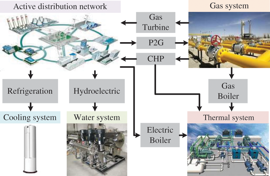
Figure 1: IEADN schematic representation
The operational model of an ADN providing electrical power supply can be expressed as [25]:
where Pi and Qi are the active and reactive powers injected into node i, respectively; Vi and Vj are the voltage amplitude at nodes i and j, respectively; Gij and Bij are the conductors and conductivity of branch ij, respectively; and branchi represents the set of branches connected to node i. DGs (mainly PV and energy storage systems (ESSs)) are presented in ADNs to enhance the electricity supply reliability. The PV generator output power can be modeled as Eq. (2).
where PPV.max(t) is the maximum output power of the PV; G(t) and GN are the solar radiation intensities at time t and for the rated scenario, respectively; α is the PV temperature factor; T(t) and TN are the temperatures at t and the rated scenario, respectively; T0 is the reference temperature; and PPV.N is the rated power of the PV. ESSs are used to smooth out the DG fluctuations and serve as backup power sources. The operational state of an ESS can be expressed as Eq. (3).
where SoC(t + 1) and SoC(t) are the states of charge at times t + 1 and t, respectively; ηch and ηdis are the charge and discharge efficiencies, respectively; Pch and Pdis are the charge and discharge powers, respectively; and Δt is the time interval.
The IEADN system requires a large number of energy-coupling equipment. The coupling equipment between the ADNs and the gas system mainly consists of power-to-gas (P2G) units, combined heat and power (CHP) units, and gas turbines (Fig. 1). The CHP units primarily convert natural gas into electrical and thermal power to be supplied to the grid loads. This process can expressed as Eq. (4).
where Pge and Pgh are the output electrical and thermal power of the CHP, respectively; Lge and Lgh are the gas loads converted into electricity and heat, respectively; and ηge and ηgh are the electricity and heat transformation efficiencies, respectively. The energy exchange between the ADNs and the cooling system occurs through refrigeration, with the operational model expressed as Eq. (5).
where Pec is the cooling power; Lec is the electrical load; and ηec is the transforming efficiency to cooling.
The IEADN gas supply is based on pipeline transmission [26], which is composed of the
(i) pipeline flow model, expressed as
where Ag is the gas system topological structure; Fg is the pipe flow matrix; Sg and Lg are the gas source and load, respectively; kij is a constant related to the internal diameter, length, efficiency, and natural gas compression factor of the pipeline ij; and πi and πj are the pressures at nodes i and j, respectively; and
(ii) compressor model, expressed as
where Lcom is the compressor power for electricity consumption; B is a constant to reflect the compressor temperature and efficiency; Z is the compression factor constant; and Fcom is the flow through the compressor.
The IEADN thermal system uses water as the work mass [27], which includes the
(i) heat model, expressed as
where Lhi is the thermal power at node i; Cp is the specific heat capacity of water; Tsi and Toi are the water inflow and outflow temperatures at node i, respectively; Ta is the environmental temperature; λ is the heat transfer index of the heat network pipes; lij is the length of pipe ij; and mi expresses the flow of pipe ij; and
(ii) hydraulic model, expressed as
where Aw is the node-branch correlation matrix for island heat networks; Fw is the matrix describing the water flow, Fij, in pipe ij; and Sw is the water source power.
3 Modified OPA Model for IEADNs for Cascading Fault Path Prediction
The traditional OPA model is based on a blackout model, which adopts a sequence of linear programs to describe the load shed induced by the power system cascading faults [28]. The proposed modified OPA model, however, uses a two-layer structure (Fig. 2). The time-series-based upper-layer model portrays the IEADN cascading fault path by updating the operating state of each component at different moments. The power-flow-based lower-layer model calculates the power flow distribution in accordance with the various IEADN component failures.
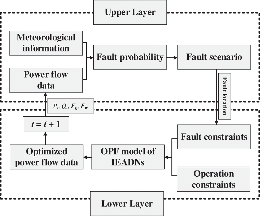
Figure 2: Interactions between the upper and lower-layers of the modified OPA model
Based on the extreme weather meteorological parameters, the IEADN fault probability generated the typical fault scenario, which was set as the initial fault of the proposed OPA model (Fig. 3). Then, the combined component fault probability, P, was obtained, and the faulty component was determined until the extreme weather moved away from the IEADN.
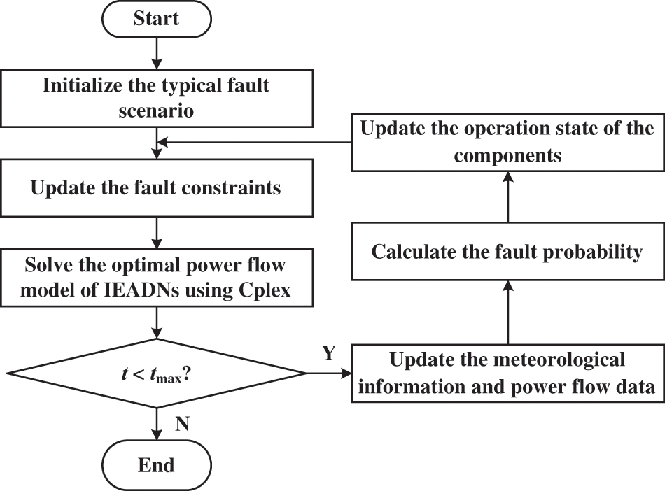
Figure 3: Workflow of the proposed OPA model
3.1 Upper-Layer Model for Fault Scenario Selection
3.1.1 Component Fault Probability during Typhoons
Using the Batts model, the wind speed can be expressed as [29]
where v is the typhoon velocity, tangential in direction to the analog circle; Rmax is the typhoon radius at its maximum velocity; vRmax is the maximum typhoon velocity; and r is the distance between the study location of the typhoon location and its center point. The pressure applied on the lines, pl, and poles, pp, can be calculated using the wind speed.
where D is the line diameter; μ is a constant inflecting the line type; θ is the angle between the wind and the line; q is the line mass; g is the gravitational acceleration; D0 and Dp are the top and root diameters of the pole, respectively; and hp is the pole height.
From Eq. (13), the component fault probability, Pfault, due to the typhoon can be obtained as
where fp is the component strength probability density; and p and pr are the components of bearable pressure and real pressure p or pp. Furthermore, the operational failure probability, Pflow, caused by flow transgression can be defined as Eq. (14).
where I and Imax are the operation current and maximum current, respectively, and ε is the current margin. To forecast the IEADN cascading fault paths under extreme weather, using Eqs. (13) and (14), the combined component fault probability, P, can be defined as
3.1.2 Typical Fault Scenario during Typhoons
The IEADN information entropy, E, reflects the probability of a fault scenario occurrence, computed using the combined component fault probability, P, as Eq. (16).
and
where Tw is the typhoon duration above the IEADNs; and zi,t = 1 implies the occurrence of a fault at branch i at time t (for each branch i, there exists at most one instance where zi,t = 1). Each fault scenario corresponds to i zi,t vectors and an entropy, E.
3.2 Lower-Layer Model for Optimal Power Flow
To improve the IEADN power flow under extreme events, the objective function, F, of the lower-layer was modeled considering the flow transgression rate, energy coupling element utilization, and load recovery rates of different energy networks as Eq. (18).
where ω1–3 are the weights of different sub-objective functions; m and n are the number and quantity of the energy coupling equipment, respectively; and Li and LiN are the supplied and rated loads, respectively.
3.2.2 Constraints of the Lower-Layer Model
1) Distribution network operation
where PG and PPV are the powers of the traditional generator and PV units, respectively; Pbranch is the power flow in the branches; Ae is the ADN structure; Pco is the power of the coupling components; Le is the electric load; and PG.max, PPV.max, Pbranch.max, Pdis.max, Le.max, and Lch.max are the maximum values of the corresponding parameters.
2) Gas system operation
The gas network operation mainly satisfies the gas flow equation, gas load shedding constraint, gas pressure constraint, and the pipe limit, and can be expressed as Eq. (20).
where ΔLg is the gas load; π is the pressure at all the gas system nodes, with πmax and πmin being the maximum and minimum values of π; and Fg.max is the maximum pipe flow.
3) Thermal system operation
where ΔLw is the water load; p is the pressure at all the water system nodes, with pmax and pmin being the maximum and minimum values of p, respectively; Lh is the matrix for Lhi, with Lh.max being its maximum; and T is the matrix for Tsi and Toj; with Tmax and Tmin containing the maximum and minimum values of T.
4) Cooling system
For the IEADNs, the cooling (air-conditioning) loads can expressed as Eq. (22).
where Pec is the matrix for Pec, with Pec.max containing its maximum value.
5) Extreme events
where Ae.ij is an adjacency matrix element; Le.i.max is the maximum electrical load at node i; Pij and Pj are the component fault probabilities for branch ij and node j, respectively; and τ is a random number.
In Eqs. (19)–(23), the inequalities are linear constraints and can be solved using exact algorithms based on mathematical principles [30]. However, the equality constraints describing the power flow are second-order cone constraints (SOCCs), which cannot be solved directly by using exact algorithms. The second-order cone relaxation method was used to transform equality SOCCs into inequality SOCCs [31]. After the transformation, the OPF model of the IEADNs could be solved via Yalmip and CPLEX. CPLEX primarily uses a barrier optimizer that exploits a primal-dual logarithmic barrier algorithm to generate a sequence of strictly positive primal and dual solutions to the given problem [32]. Unlike heuristic algorithms that use stochastic generation and iterative optimization, the primal-dual logarithmic barrier algorithm solves second-order cone problems by generating a Lagrangian function and obtaining its maximum/minimum. This method is often better suited and advantageous for large-scale problems [33].
4.1 IEADNs Based on the Modified IEEE 33-Node System
We established an IEADN (Fig. 4) based on the modified IEEE 33-node system [34] and compared it with the 7-node gas system [35] and the modified 32-node thermal system [36]. The test case was modeled on a PC with Intel Core i7-9700 CPU 3.00 GHz and 16 GB memory, with MATLAB 2020a used as the testing environment. A CHP unit was connected to node 7 as the gas load, which provided electrical and thermal power to nodes 14 and 23 of the electrical and thermal systems, respectively.
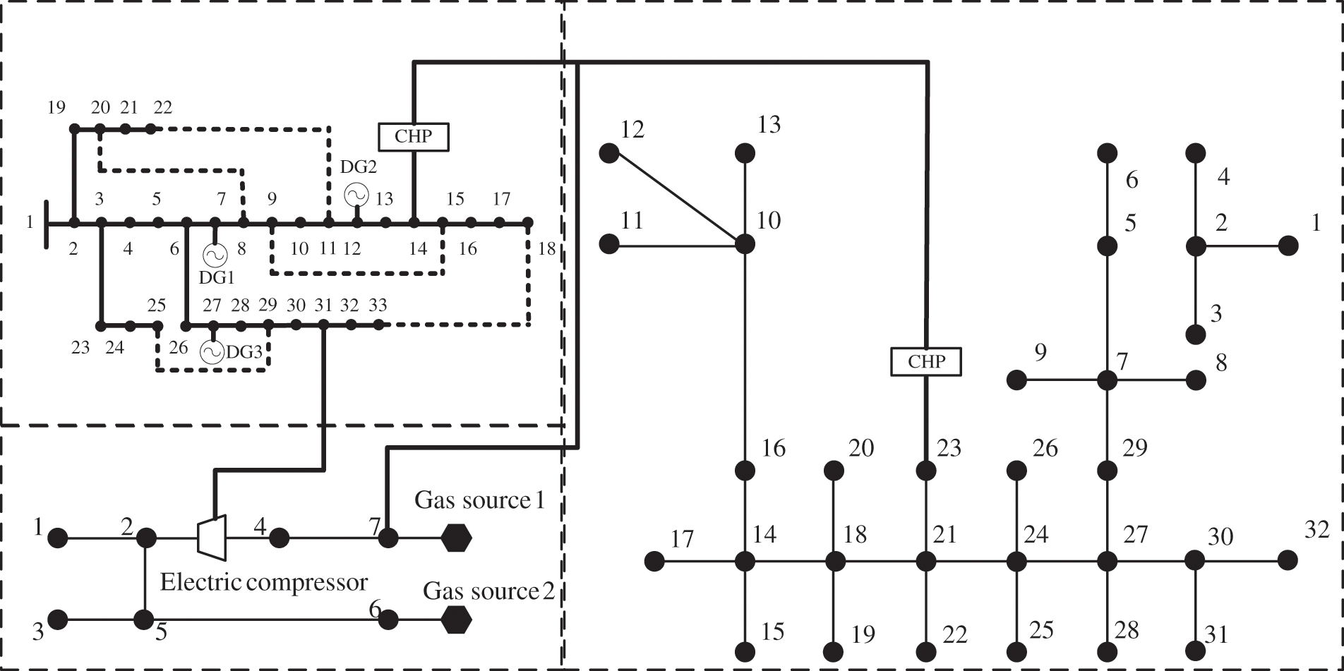
Figure 4: IEADNs based on the modified IEEE 33-node system
The Batts model simulated a typhoon attack on the IEADNs, with Rmax and Vmax set to the initial values of 50 km and 144 km/h, respectively. The IEADN fault probability during the day was obtained (Fig. 5). Over 90% of the fault scenarios caused by the typhoon event exhibited 60 ≤ E ≤ 120. When the fault occurred at branches 11, 12, 19, and 21, we obtained E = 80.24 and determined the maximum probability density (Fig. 6).
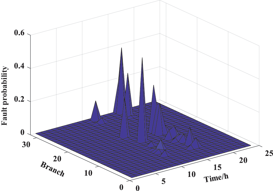
Figure 5: Fault probability distribution for the IEADN nodes
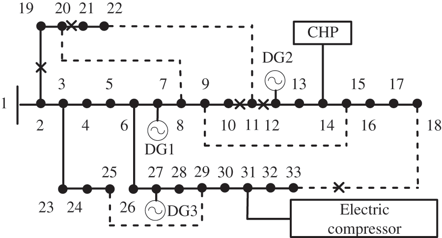
Figure 6: Typical IEADN fault scenario
According to Fig. 5, for t = 00:00–10:00, the IEADNs were in a normal operational state. From t = 11:00, the typical fault scenario was taken to be the initial fault state (Fig. 6). The cascading fault path, predicted using the improved OPA model, spread according to the movement of the typhoon (Fig. 7). As the typhoon moved towards nodes 29–31, the branches in between were damaged.
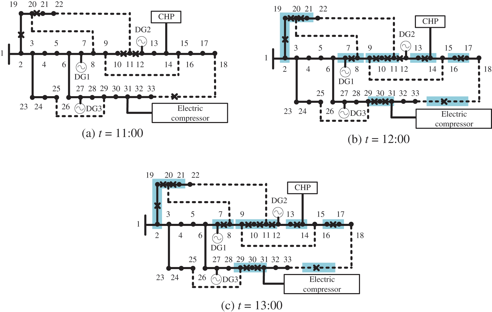
Figure 7: IEADN cascading fault paths at t = (a) 11:00; (b) 12:00; and (c) 13:00
The modified double-layer OPA model was compared to the traditional OPA model in terms of typhoon response and load recovery. In the network reconfiguration of the proposed OPA model, the contact switches on branches 33, 34, and 35 were connected to recover the outage loads at nodes 8, 19, and 20 (Fig. 8). The traditional model did not reflect this process and the loads were not recovered.
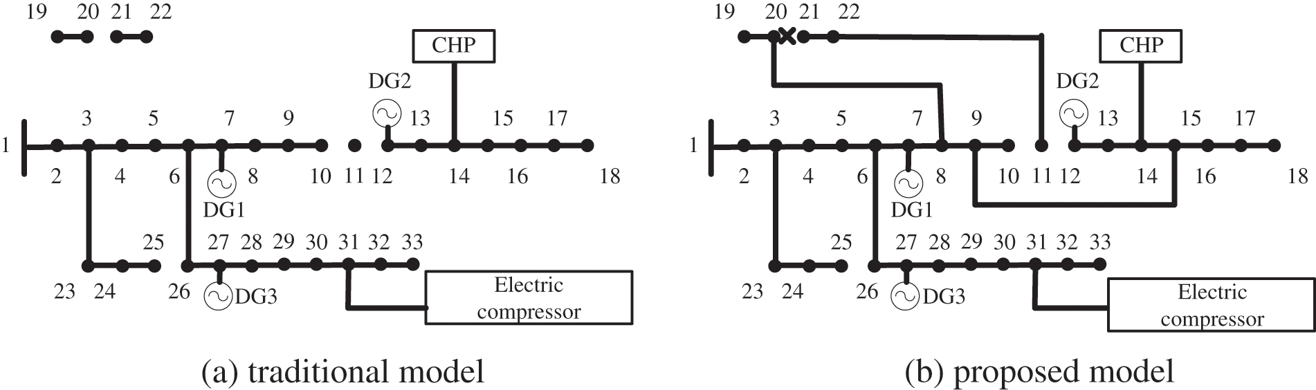
Figure 8: IEADN network structure during the typhoon at t = 11:00 using the (a) traditional and (b) improved OPA models
Detailed values of the IEADN load recovery rates were obtained (Fig. 9; Table 1). Minimum recovery rates of 53% and 42% were observed for the proposed and traditional OPA models, respectively, at t = 12:00 and 18:00. Simultaneously, a 26.2% performance enhancement was observed for the proposed OPA model compared to the traditional one.
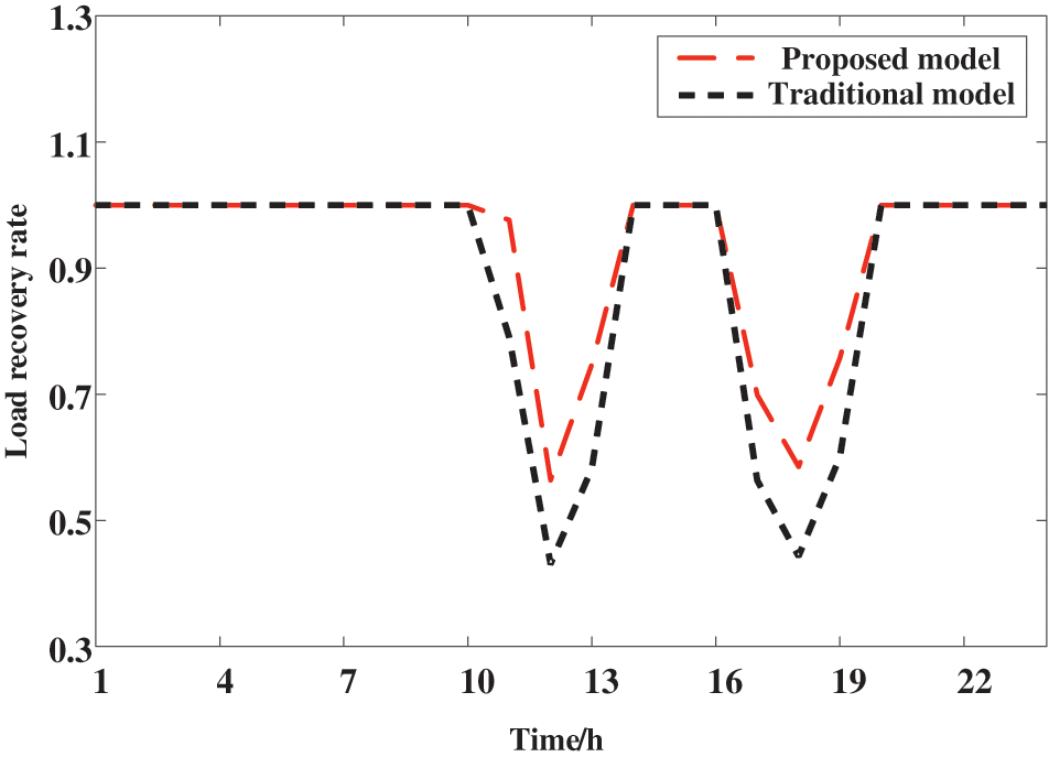
Figure 9: IEADN load recovery rates for the traditional and proposed OPA models
4.2 IEADN for Practical Large-Scale Hydroelectric Units
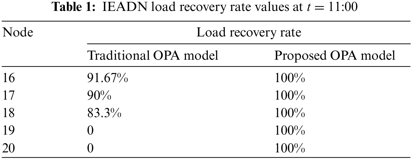
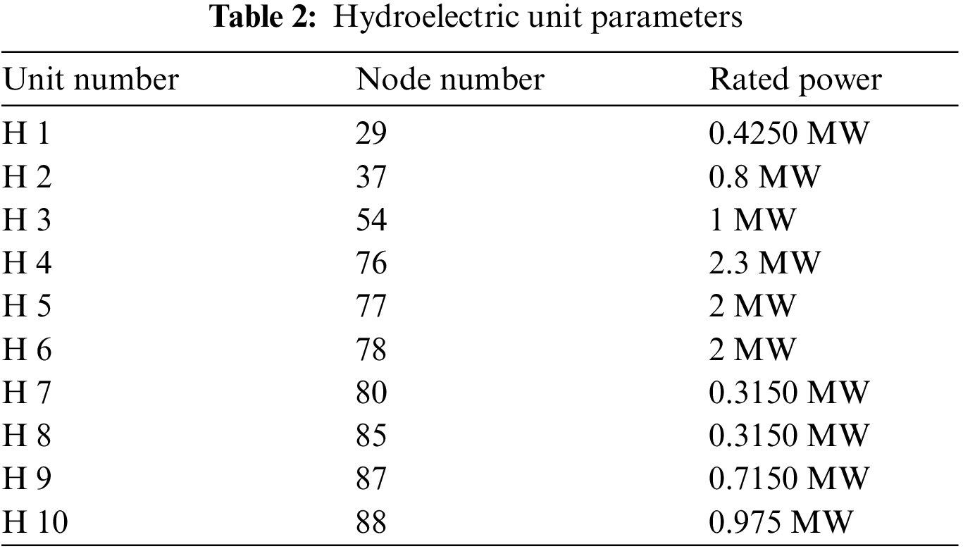
To verify the effectiveness of the proposed OPA model for practical systems, we established an IEADN with a 98-node distribution system based on the actual distribution network in a city for large-scale hydroelectric units (Fig. 10). The hydraulic sub-system consisted of 10 hydroelectric units (Table 2).
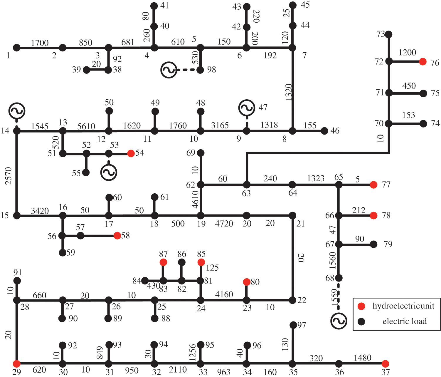
Figure 10: IEADN based on a real distribution network for large-scale hydroelectric units
Using the meteorological information for the typhoon (Table 3) and the wind speeds at each IEADN node during the day (Fig. 11), we inferred that nodes 8, 9, 67, 68, and 70–75 were the most affected. Node 8 experienced a maximum wind speed of 69 km/h at 09:00–11:00; it was the first node to peak, and hence, was established as the typhoon starting coordinate. As the typhoon path was farther away from nodes 1–7 and 90–100, these locations experienced relatively lower wind speeds, which was consistent with the typhoon model.
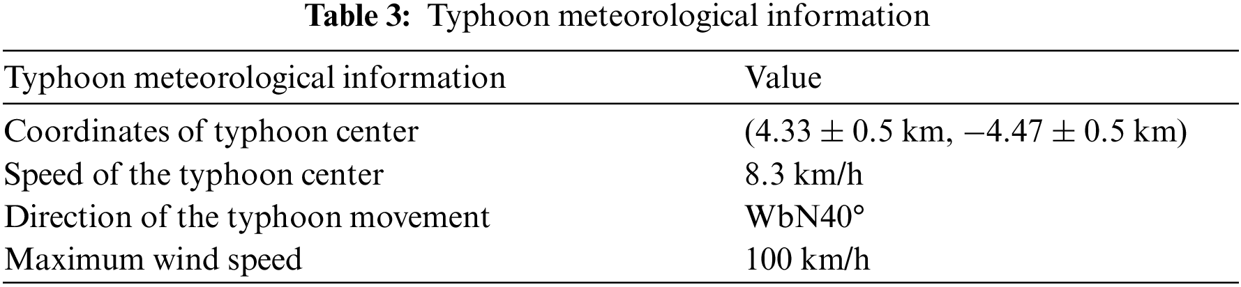
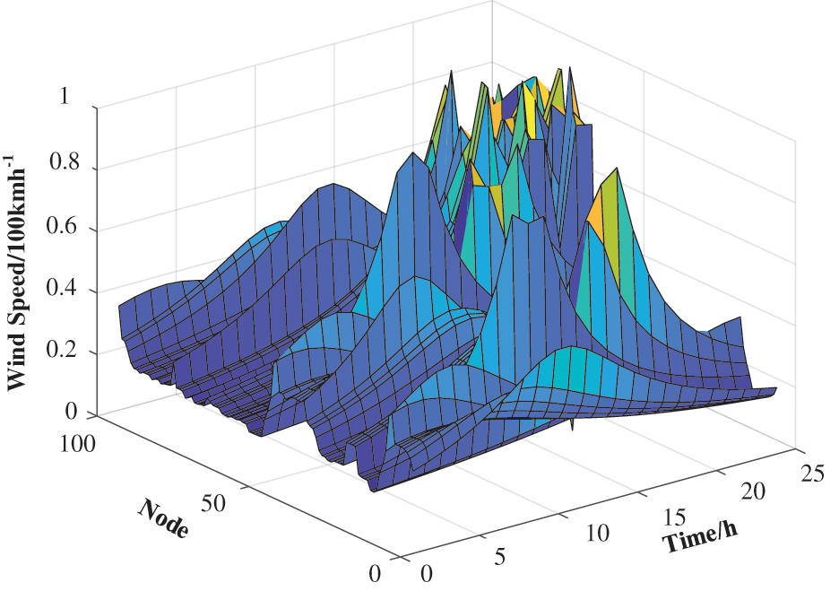
Figure 11: Wind speeds at each IEADN node
The fault probability computation for each IEADN node (Fig. 12) revealed an upward trend for branches 8 and 9, with an increase from 0% to 70% at 06:00–10:00, consistent with the wind speeds at these locations. At ~15:00, branches 45–55 experienced a very high fault probability, for a wind speed of ~90 km/h. After simulating a typhoon attack on the IEADNs with the initial coordination in the range of (4.33 ± 0.5 km), (–4.47 ± 0.5 km), we computed the E-values for each fault scenario.
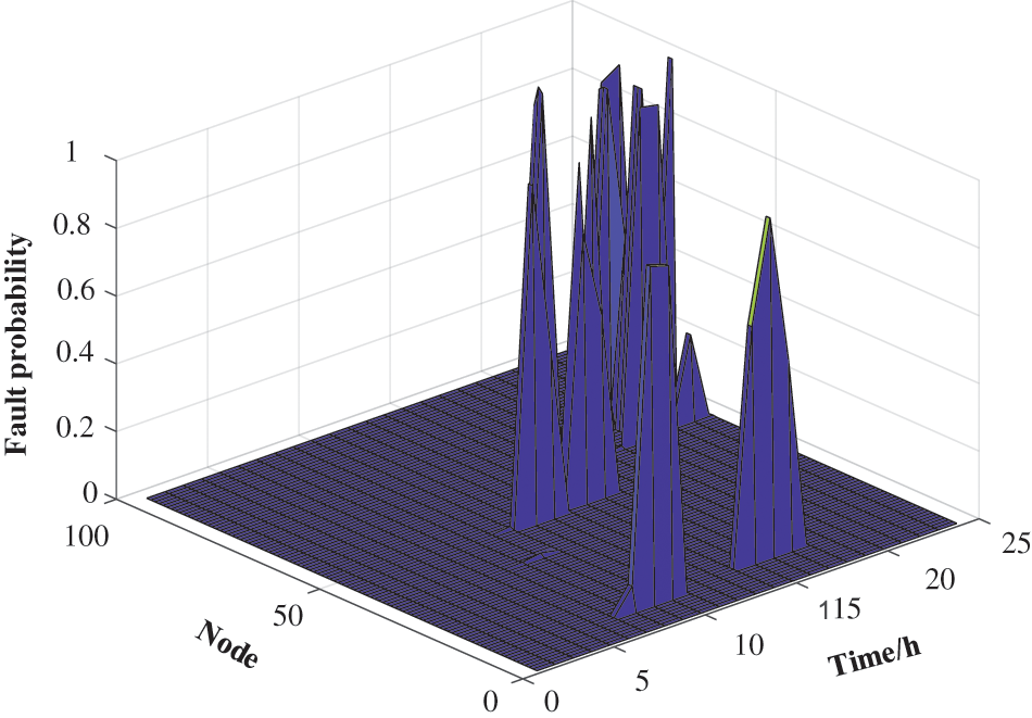
Figure 12: Fault probability at each IEADN node
The E-value probability density for 90% of the fault scenarios was distributed in the range of 3484.0–3487.0. Based on the simulation results, for the fault in branches 9 and 10, we computed E = 3485.5 for the typical fault scenario. Compared to the 33-node-based IEADN, the nodes and branches of the IEADN for large-scale hydroelectric units were found to be more decentralized, verifying the efficiency of the proposed model for larger IEADNs (Fig. 13).
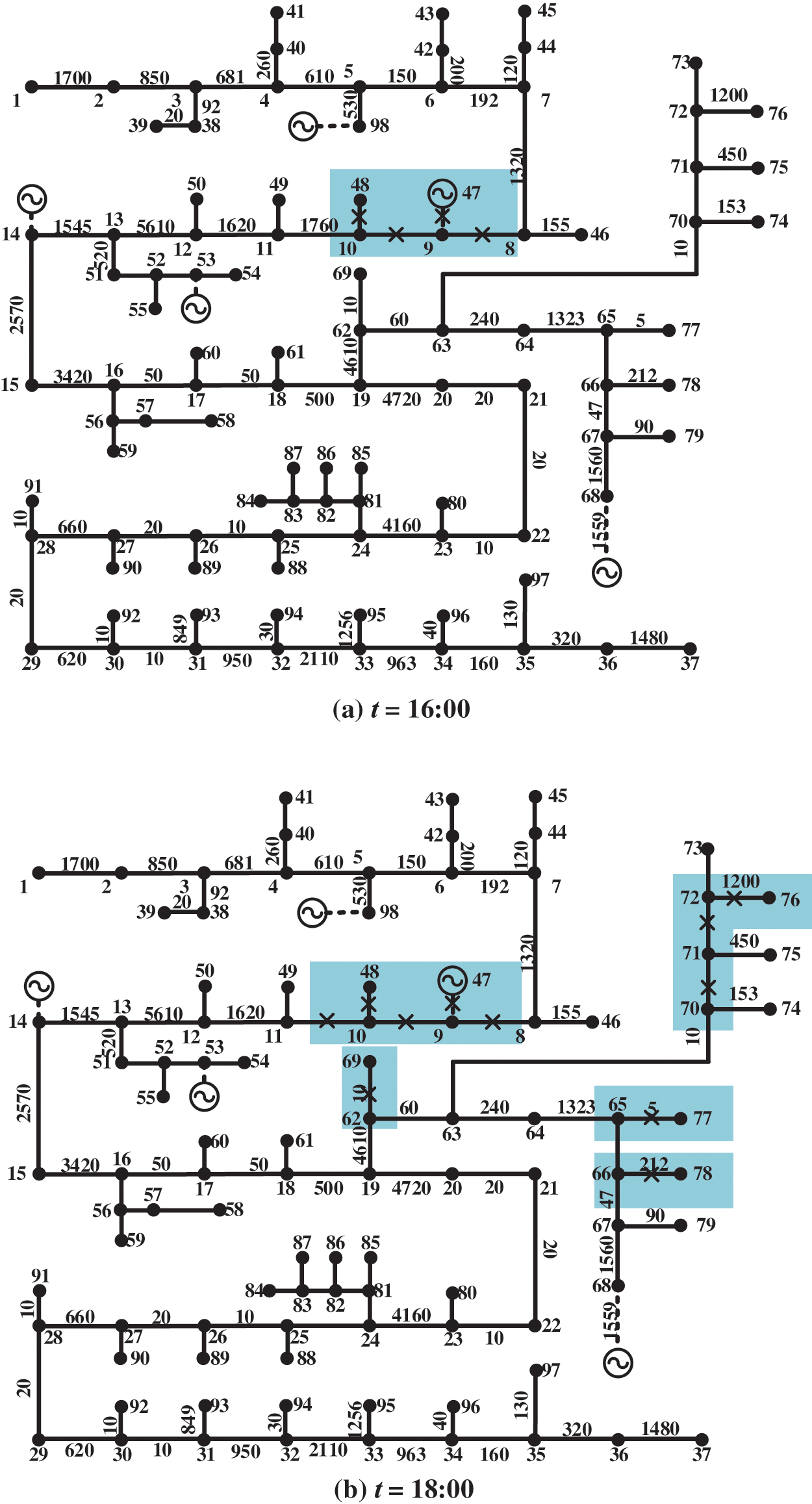
Figure 13: Cascading fault paths for the IEADNs at t = (a) 16:00 and (b) 18:00
For the proposed OPA model, the coupling equipment utilization rate reached up to 0.60 for all periods, with a minimum value of 0.76 (Fig. 14). In contrast, for the traditional OPA model, the minimum coupling equipment utilization rate was ~0.58. This confirmed that during the IEADN operation process, the modified OPA model was more capable of using the energy coupling equipment to withstand extreme events compared to the traditional one.
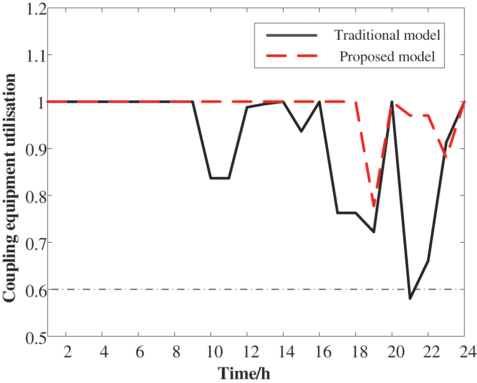
Figure 14: IEADN coupling equipment utilization comparison
For the modified OPA model, the load recovery rate was >0.90, but it remained <0.80 for the traditional model (Fig. 15). It was worth noting that the IEADNs with higher numbers of coupling equipment had a better load recovery rate compared to the 33-node-based IEADN, further confirming the practical applicability of the proposed model.
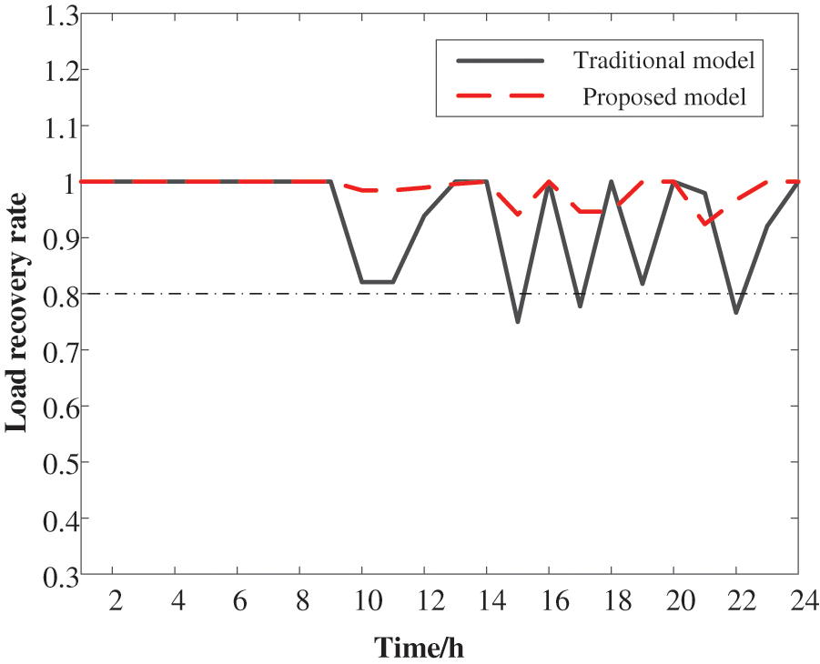
Figure 15: IEADN load recovery rate comparison
To test the performance of the proposed model for several thousands of variables, the IEADNs were expanded to a system with 196 nodes and 195 branches. The voltage, phase angle, load point active and reactive powers, coupling equipment output power, and the power transformed at the branches composed a total of 1059 variables. The cascading fault path predictions for the expanded IEADNs revealed that the initial faults were mainly centered at nodes 117, 118, 130, 131, 164, 176, 192, and 193 (lower right-hand corner of Fig. 16). As the typhoon traversed, the faults were transferred to nodes 10, 48, 71, 75, 110, 111, 148, 149, and 150 (central part of Fig. 16), consistent with the typhoon movements.
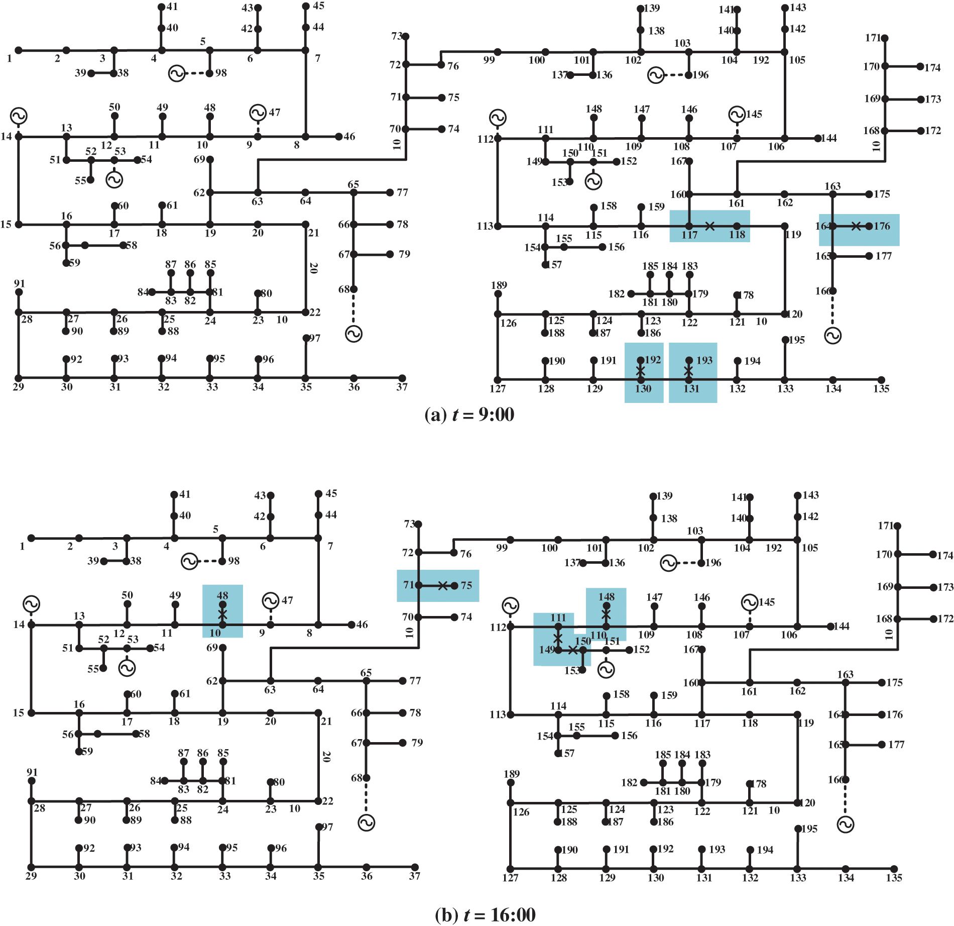
Figure 16: Cascading fault paths of the expanded IEADNs at t = (a) 09:00 and (b) 16:00
4.3 IEADNs Based on Concentrated Distribution Networks
To verify the proposed model for practical IEADNs with more concentrated structures, along with large-scale DGs and energy systems, we constructed a model based on the actual industrial park (Fig. 17; Table 4). We then simulated a typhoon (–8 km, –5 km) attack on the established IEADN structure (nodal wind speeds shown in Fig. 18). During the attack, nodes 5–15 and 55–60 were the most affected, with wind speeds >60 km/h. The maximum wind speed observed at node 53 was vRmax = 89 km/h at 09:00–11:00. Meanwhile, as the typhoon was farther away from nodes 15–25, the wind speed at these locations was <50 km/h.
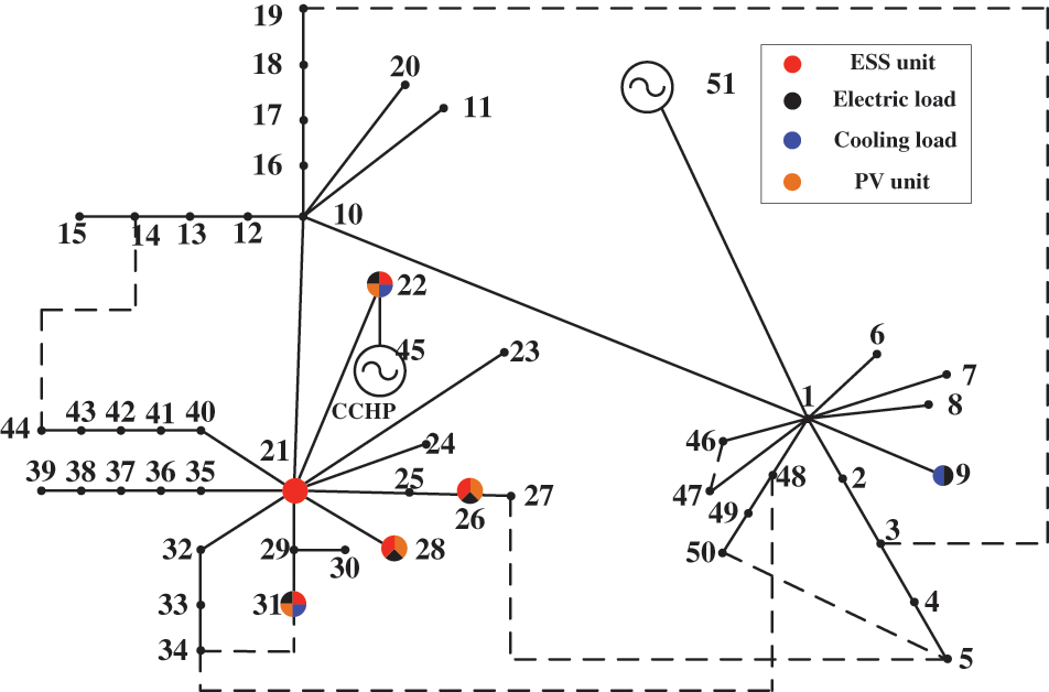
Figure 17: IEADN structure based on the industrial park
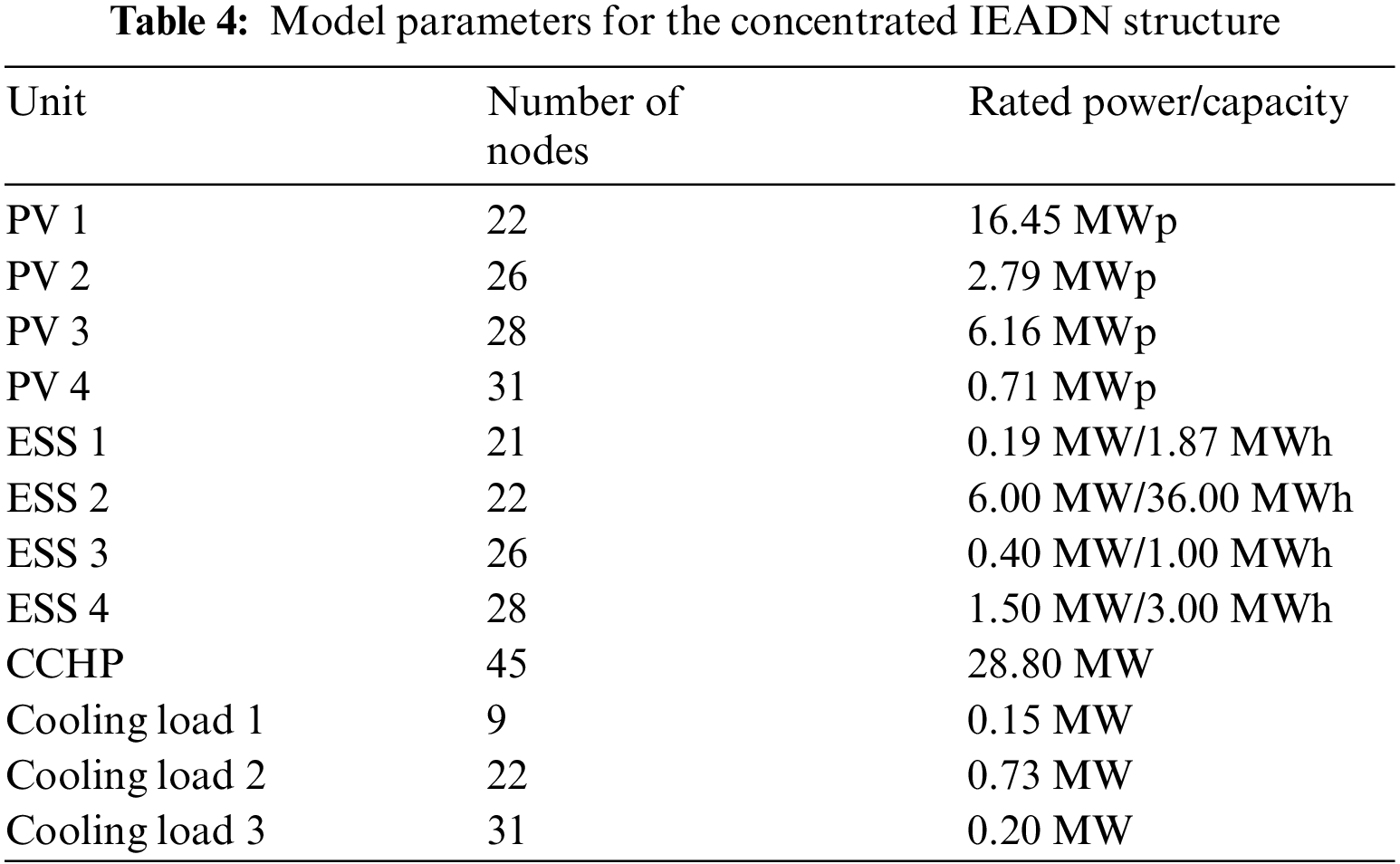
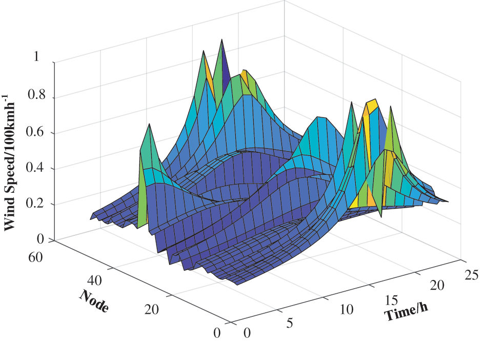
Figure 18: Wind speeds at each IEADN node
At t = 00:00–03:00, node 35 experienced wind speeds of 58 km/h, and the fault probability reached a maximum value of 0.79 (Fig. 19). Meanwhile, the maximum fault probabilities for nodes 1–10, 52, and 53 occurred between 11:00–20:00. Similarly, when branches 26, 49, and 54 were found to experience the typical failure scenario, we computed E = 3527.5.
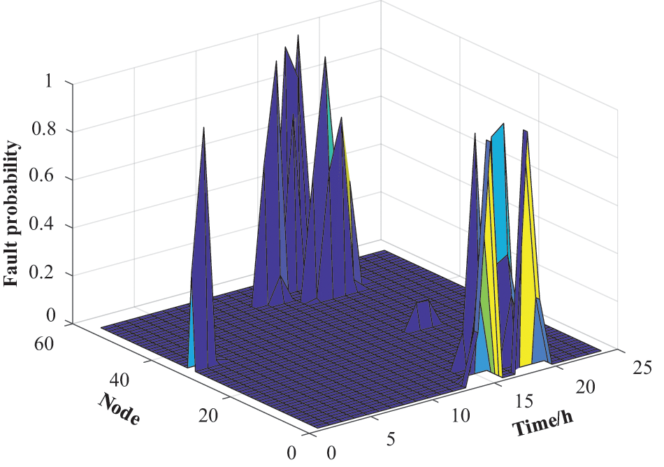
Figure 19: Fault probability density for the concentrated IEADN nodes
The typhoon began affecting the concentrated IEADN structure from 05:00 onwards (Fig. 20). Although node 35 had a high fault probability at t = 00:00–03:00, no multi-fault scenarios were observed. The cascading fault had an apparent tendency to spread from left to right on the grid, similar to the typhoon movement path. Additionally, by analyzing the number of faults, it could be concluded that the IEADNs with more concentrated structures are easily influenced by the typhoon.
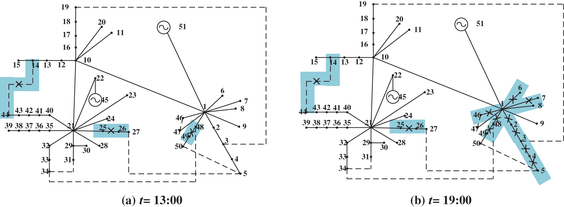
Figure 20: Cascading fault paths for the concentrated IEADN structure at t = (a) 13:00 and (b) 19:00
Under the proposed OPA model, the intraday full-time load recovery rate reached up to 0.93 compared to only 0.75 for the traditional model (Fig. 21). The load recovery rate improved significantly throughout the operation process, reaching a maximum value of 24% and illustrating the excellent performance of the proposed OPA model. The cooling load operation state of the concentrated IEADN structure had two apparent instances of decrease at 16:00 and 19:00–20:00. This phenomenon was owing to the proposed OPA model being built to prioritize electrical load recovery. As a result, the cooling load powers were deliberately controlled. Hence, the proposed OPA model could effectively repair faults by prioritizing electrical loads and slightly decreasing the cooling load (Fig. 22).
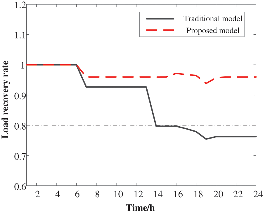
Figure 21: Load recovery rate comparison for the concentrated IEADN structure
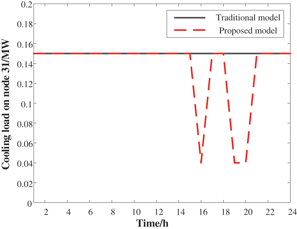
Figure 22: Cooling load operation state comparison for the concentrated IEADN structure
To handle uncertainties and analyze model sensitivity, we simulated more typhoon attacks in the range of (−8.0 ± 0.5 km, −5.0 ± 0.5 km) on the IEADNs. Each line in Fig. 23 represents a fault probability curve under a typhoon. The influenced nodes under each typhoon in the abovementioned range were highly consistent. The nodal fault probabilities exhibited differences due to the range and the speed of the typhoons. The above simulations verified the robustness of the proposed model.
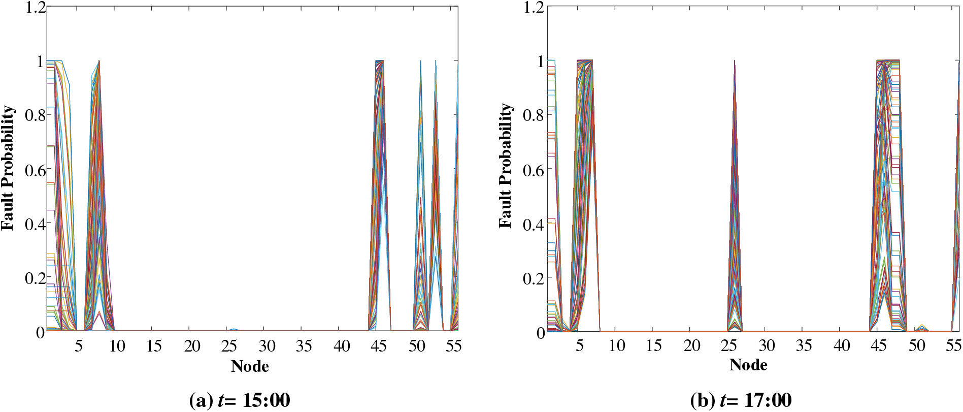
Figure 23: Fault probability comparison at each IEADN node under different typhoons at t = (a) 15:00 and (b) 17:00
In this study, we proposed an improved OPA model to predict IEADN cascading fault paths during typhoons. We established the modified OPA model and its solution scheme, and tested its validity and practical applicability in comparison to the traditional OPA model. The major conclusions of this work are summarized as follows:
1) The proposed OPA model can effectively forecast the IEADN cascading fault paths, accurately corresponding to typhoon development and fault probability features. The changes in multiple faults at different instances were clarified.
2) The novel OPA model was validated for different types of IEADNs. The IEADNs with concentrated structures are more likely to be influenced by typhoons. By using the improved OPA model, the IEADNs with large energy systems can more effectively repair faults.
3) The improved OPA model outperforms the traditional one in terms of increased coupling equipment utilization (by 31%) and load recovery rate (by >24%) of the IEADNs. This model achieves favorable cooperative recovery.
Consequently, the validity and suitability of the proposed model are demonstrated for practical conditions. Future works will be aimed at analyzing resource synergy and optimal allocation methods for multiple energy systems to enhance IEADN resilience.
Acknowledgement: The authors acknowledge the support of Guangzhou Power Supply Bureau, Guangdong Power Grid Co., Ltd.
Funding Statement: This work was supported by the Science and Technology Project of China Southern Power Grid Co., Ltd. under Grant GDKJXM20222357.
Author Contributions: The authors confirm their contribution to the paper as follows: The study conception and design: Yue He, Yaxiong You, Lei Chen, and Zhian He. Data collection: Yue He, Haiying Lu, Lei Chen, and Yuqi Jiang. Analysis and interpretation of results: Yue He, Lei Chen, and Hongkun Chen. Draft manuscript preparation: Yue He, Lei Chen, Yaxiong You, and Zhian He. All authors reviewed the results and approved the final version of the manuscript.
Availability of Data and Materials: Data supporting this study are included within the article.
Ethics Approval: Not applicable.
Conflicts of Interest: The authors declare that they have no conflicts of interest to report regarding the present study.
References
1. M. A. Mohamed, T. Chen, W. Su, and T. Jin, “Proactive resilience of power systems against natural disasters: A literature review,” IEEE Access, vol. 7, pp. 163778–163795, Nov. 2019. doi: 10.1109/ACCESS.2019.2952362. [Google Scholar] [CrossRef]
2. K. Sandhya, T. Ghose, D. Kumar, and K. Chatterjee, “PN inference based autonomous sequential restoration of distribution system under natural disaster,” IEEE Syst. J., vol. 14, no. 4, pp. 5160–5171, Dec. 2020. doi: 10.1109/JSYST.2020.2994585. [Google Scholar] [CrossRef]
3. Y. Du, Y. Liu, Y. Yan, and X. Jiang, “Disaster damage assessment of distribution systems with incomplete and incorrect information,” IEEE Trans. Power Del., vol. 38, no. 2, pp. 889–901, Apr. 2023. doi: 10.1109/TPWRD.2022.3200669. [Google Scholar] [CrossRef]
4. Z. Tan, Y. Ren, H. Li, W. Ren, X. Zhou and M. Zeng, “Data mining based integrated electric-gas energy system multi-objective optimization,” Energy Eng., vol. 119, no. 6, pp. 2607–2619, Feb. 2022. doi: 10.32604/ee.2022.019550. [Google Scholar] [CrossRef]
5. M. Li et al., “Two-stage optimal scheduling of community integrated energy system,” Energy Eng., vol. 121, no. 2, pp. 405–424, Jan. 2024. doi: 10.32604/ee.2023.044509. [Google Scholar] [CrossRef]
6. W. Ji, T. Tu, and N. Ma, “A novel defender-attacker-defender model for resilient distributed generator planning with network reconfiguration and demand response,” Energy Eng., vol. 121, no. 5, pp. 1223–1243, Apr. 2024. doi: 10.32604/ee.2024.046112. [Google Scholar] [CrossRef]
7. K. Wang et al., “Resilience-oriented load restoration method and repair strategies for regional integrated electricity-natural gas system,” Energy Eng., vol. 121, no. 4, pp. 1091–1108, Mar. 2024. doi: 10.32604/ee.2023.044016. [Google Scholar] [CrossRef]
8. X. Chen, J. Qiu, L. Reedman, and Z. Dong, “A statistical risk assessment framework for distribution network resilience,” IEEE Trans. Power Syst., vol. 34, no. 6, pp. 4773–4783, Nov. 2019. doi: 10.1109/TPWRS.2019.2923454. [Google Scholar] [CrossRef]
9. J. Li, X. Xu, Z. Yan, H. Wang, M. Shahidehpour and Y. Chen, “Coordinated optimization of emergency response resources in transportation-power distribution networks under extreme events,” IEEE Trans. Smart Grid, vol. 14, no. 6, pp. 4607–4620, Nov. 2023. doi: 10.1109/TSG.2023.3257040. [Google Scholar] [CrossRef]
10. Y. Wu, Z. Lin, T. Huang, Y. Chen, Y. Ru and J. Chen, “Resilience enhancement for urban distribution network via risk-based emergency response plan amendment for ice disasters,” Int. J. Electr. Power Energy Syst., vol. 141, pp. 108183, Oct. 2022. [Google Scholar]
11. Z. Li, W. Tang, X. Lian, X. Chen, W. Zhang and T. Qian, “A resilience-oriented two-stage recovery method for power distribution system considering transportation network,” Int. J. Electr. Power Energy Syst., vol. 135, no. 7, pp. 107497, Feb. 2022. doi: 10.1016/j.ijepes.2021.107497. [Google Scholar] [CrossRef]
12. L. Chen et al., “Impact of cascading failure on power distribution and data transmission in cyber-physical power systems,” IEEE Trans. Netw. Sci. Eng., vol. 11, no. 2, pp. 1580–1590, Mar. 2024. doi: 10.1109/TNSE.2023.3325539. [Google Scholar] [CrossRef]
13. W. Liu, Q. Yao, Q. Shi, Y. Xue, and Y. Wang, “Risk assessment of cascading failure of distribution network with flexible multi-state switch,” Int. J. Electr. Power Energy Syst., vol. 142, pp. 108290, Nov. 2022. [Google Scholar]
14. Y. Bai, X. Gu, S. Li, and K. Liu, “Coordinated restoration method of transmission and distribution network considering distribution network fault repair scenario,” Int. J. Electr. Power Energy Sys., vol. 151, pp. 109153, Sep. 2023. doi: 10.1016/j.ijepes.2023.109153. [Google Scholar] [CrossRef]
15. X. Wang, F. Xue, Q. Wu, S. Lu, L. Jiang and Y. Hu, “Evaluation for risk of cascading failures in power grids by inverse-community structure,” IEEE Internet Things J., vol. 10, no. 9, pp. 7459–7468, May 2023. doi: 10.1109/JIOT.2022.3189001. [Google Scholar] [CrossRef]
16. X. Gao, M. Peng, and C. Tse, “Cascading failure analysis of cyber-physical power systems considering routing strategy,” IEEE Trans. Circuits Syst. II: Exp. Briefs, vol. 70, no. 1, pp. 136–140, Jan. 2023. doi: 10.1109/TCSII.2021.3071920. [Google Scholar] [CrossRef]
17. Z. Du, J. Chen, H. Zhao, W. Zhang, and Y. Zhang, “Routing optimization method of cyber-energy system considering cross-space cascading fault handling process,” Int. J. Electr. Power Energy Syst., vol. 144, pp. 108574, Jan. 2023. doi: 10.1016/j.ijepes.2022.108574. [Google Scholar] [CrossRef]
18. C. Chen, S. Ma, K. Sun, X. Yang, C. Zheng and X. Tang, “Mitigation of cascading outages by breaking inter-regional linkages in the interaction graph,” IEEE Trans. Power Syst., vol. 38, no. 2, pp. 1501–1511, Mar. 2023. doi: 10.1109/TPWRS.2022.3175481. [Google Scholar] [CrossRef]
19. R. Ma, S. Basumallik, and S. Eftekharnejad, “Controlled islanding resilience with high penetration of renewable energy resources,” IEEE Trans. Sustain. Energy, vol. 14, no. 2, pp. 1312–1323, Apr. 2023. doi: 10.1109/TSTE.2022.3214421. [Google Scholar] [CrossRef]
20. Y. Yang et al., “An event-triggered hybrid system model for cascading failure in power grid,” IEEE Trans. Autom. Sci. Eng., vol. 19, no. 3, pp. 1312–1325, Jul. 2022. doi: 10.1109/TASE.2022.3169069. [Google Scholar] [CrossRef]
21. Y. Dai, M. Noebels, R. Preece, M. Panteli, and I. Dobson, “Risk assessment and mitigation of cascading failures using critical line sensitivities,” IEEE Trans. Power Syst., vol. 39, no. 2, pp. 3937–3948, Mar. 2024. doi: 10.1109/TPWRS.2023.3305093. [Google Scholar] [CrossRef]
22. Q. Wang, Y. Xiao, H. Tan, and M. Mohamed, “Day-ahead scheduling of rural integrated energy systems based on distributionally robust optimization theory,” Appl. Therm. Eng., vol. 246, pp. 123001, Jun. 2024. doi: 10.1016/j.applthermaleng.2024.123001. [Google Scholar] [CrossRef]
23. H. Tan, Z. Li, Q. Wang, and M. Mohamed, “A novel forecast scenario-based robust energy management method for integrated rural energy systems with greenhouses,” Appl. Energy, vol. 330, pp. 120343, Jan. 2023. doi: 10.1016/j.apenergy.2022.120343. [Google Scholar] [CrossRef]
24. Z. Li, Y. Xia, Y. Bo, and W. Wei, “Optimal planning for electricity-hydrogen integrated energy system considering multiple timescale operations and representative time-period selection,” Appl. Energy., vol. 362, no. 3, pp. 122965, May 2024. doi: 10.1016/j.apenergy.2024.122965. [Google Scholar] [CrossRef]
25. R. Sadnan and A. Dubey, “Distributed optimization using reduced network equivalents for radial power distribution systems,” IEEE Trans. Power Syst., vol. 36, no. 2, pp. 3645–3656, Jul. 2021. doi: 10.1109/TPWRS.2020.3049135. [Google Scholar] [CrossRef]
26. B. Sheykhloei, T. Abedinzadeh, L. Mohammadian, and B. Mohammadi-Ivatloo, “Optimal co-scheduling of distributed generation resources and natural gas network considering uncertainties,” J. Energy Storage, vol. 21, pp. 383–392, Feb. 2019. doi: 10.1016/j.est.2018.11.018. [Google Scholar] [CrossRef]
27. L. Wang, J. Yuan, X. Qiao, and X. Kong, “Optimal rule based double predictive control for the management of thermal energy in a distributed clean heating system,” Renew. Energy, vol. 215, pp. 118924, Oct. 2023. [Google Scholar]
28. Z. Li, G. Wu, R. Cassandro, and H. Wang, “A review of resilience metrics and modeling methods for cyber-physical power systems (CPPS),” IEEE Trans. Reliab., vol. 73, no. 1, pp. 59–66, Mar. 2024. doi: 10.1109/TR.2023.3339388. [Google Scholar] [CrossRef]
29. H. Hou et al., “Resilience enhancement of distribution network under typhoon disaster based on two-stage stochastic programming,” Appl. Energy, vol. 338, pp. 120892, May 2023. doi: 10.1016/j.apenergy.2023.120892. [Google Scholar] [CrossRef]
30. M. Cococcioni, A. Cudazzo, M. Pappalardo, and Y. Sergeyev, “Solving the lexicographic multi-objective mixed-integer linear programming problem using branch-and-bound and grossone methodology,” Commun. Nonlinear Sci. Numer. Simul., vol. 84, no. 12, pp. 105177, May 2020. doi: 10.1016/j.cnsns.2020.105177. [Google Scholar] [CrossRef]
31. L. Chen, C. Ni, J. Feng, B. Huang, H. Liu and H. Pan, “Proximity query based on second order cone programming using convex superquadrics: A static collision detection algorithm for narrow-phase,” Assem. Autom., vol. 35, no. 4, pp. 367–375, Sep. 2015. doi: 10.1108/AA-03-2015-018. [Google Scholar] [CrossRef]
32. R. Pinheiro, G. Lage, and G. Costa, “A primal-dual integrated nonlinear rescaling approach applied to the optimal reactive dispatch problem,” Eur. J. Oper. Res., vol. 276, no. 3, pp. 1137–1153, Aug. 2019. doi: 10.1016/j.ejor.2019.01.060. [Google Scholar] [CrossRef]
33. R. Barros, G. Lage, and R. Rabêlo, “Sequencing paths of optimal control adjustments determined by the optimal reactive dispatch via Lagrange multiplier sensitivity analysis,” Eur. J. Oper. Res., vol. 301, no. 1, pp. 373–385, Aug. 2022. doi: 10.1016/j.ejor.2021.11.001. [Google Scholar] [CrossRef]
34. S. Dolatabadi, M. Ghorbanian, P. Siano, and N. Hatziargyriou, “An enhanced IEEE 33 bus benchmark test system for distribution system studies,” IEEE Trans. Power Syst., vol. 36, no. 3, pp. 2565–2572, May 2021. doi: 10.1109/TPWRS.2020.3038030. [Google Scholar] [CrossRef]
35. H. Liu, C. Wang, P. Ju, Z. Xu, and S. Lei, “A bi-level coordinated dispatch strategy for enhancing resilience of electricity-gas system considering virtual power plants,” Int. J. Electr. Power Energy Syst., vol. 147, pp. 108787, May 2023. doi: 10.1016/j.ijepes.2022.108787. [Google Scholar] [CrossRef]
36. V. Srinivas, J. Wu, B. Singh, and S. Mishra, “Hybrid state-estimation in combined heat and electric network using SCADA and AMI measurements,” Int. J. Electr. Power Energy Syst., vol. 156, no. 2, pp. 109726, Feb. 2024. doi: 10.1016/j.ijepes.2023.109726. [Google Scholar] [CrossRef]
Cite This Article
 Copyright © 2024 The Author(s). Published by Tech Science Press.
This work is licensed under a Creative Commons Attribution 4.0 International License , which permits unrestricted use, distribution, and reproduction in any medium, provided the original work is properly cited.
 Downloads
 Citation Tools