A Distributed Photovoltaics Ordering Grid-Connected Method for Analyzing Voltage Impact in Radial Distribution Networks

1  Introduction

With the strategic objectives of ‘carbon peak, carbon neutralization’ and ‘new power system’ being put forward one after another, power systems have further transformed into a direction with a high proportion of new energy as the main body [1,2]. In recent years, photovoltaics has become the main force of new energy power generations, especially DPV, because of its characteristics of adapting to local conditions and balancing loads nearby, its installed capacity has ushered in explosive growth. In this context, it is an inevitable trend that county distribution networks can carry a high DPV proportion in China [3]. The structure of the county distribution network is generally radial, which supplies power to urban and rural areas under its jurisdiction. It has the characteristics of long line length and large voltage drop. The large-scale DPV connection also has higher requirements for its safe operation, especially in terms of voltage [4,5]. Therefore, in the early development stage of county DPV, it is necessary to analyze the voltage impact of large-scale DPV being connected to the radial distribution network in combination with the photovoltaics carrying capacity of each transformer district.

Scholars have done a lot of analysis on the impact of voltage changes after photovoltaic connection to the distribution network. References [6,7] show that with the increase in the proportion of photovoltaics grid-connected, the local load cannot be completely consumed, resulting in the voltage limit of the distribution network node. References [8,9] show that due to the photovoltaics connection, the distribution network becomes a multi-source power grid, and the power flow situation is more complicated, which in turn affects the voltage stability. Reference [10] analyzes the efficiency of photovoltaic inverters across the range of normal and abnormal grids on voltage impact. When DPV generation fluctuates, the distribution network will have heavy overload or even reverse power flow, which will lead to the node exceeding the limit. Reference [11] uses PSS/E to monitor the voltage of the grid-connected node of a 51 kW photovoltaic power generation system for one day. The results show that the voltage at the grid-connected node exceeds the limit during the photovoltaic power generation period. Furthermore, reference [12] gives the minimum photovoltaic output value when grid-connected node voltage exceeds the upper limit. To further analyze the power flow factors that impact the voltage change in the distribution network, references [13–16] construct the node voltage expressions based on a single radiation line. Through the comparative analysis of the expression before and after the photovoltaic connection, it can be seen that the node voltage will rise with the photovoltaics connection, and the voltage rise of each node is different. In the past, specific research methods for the phenomenon of photovoltaics connection to raise voltage were carried out. On the one hand, the intuitive results of the impact of photovoltaics on voltage under different grid-connected capacity, different grid-connected locations, and different line parameters were discussed respectively [17–19]. On the other hand, only from the inside of the DPV system, the factors and mechanism of its impact on the voltage of the distribution network are discussed [20].

Although previous studies have shown that due to differences in network structure, network parameters, and external grid-connected photovoltaics, the network node voltage will change differently, the main factors of different voltage changes in the network have not been explored. The coupling relationship between node voltage and node injection power shows that with injection powers at grid-connected nodes changing all the time caused by intermittence, randomness, and fluctuation of photovoltaic generation, node voltage also changes [21]. Therefore, it is urgent to further explore the main factors that cause different changes in the voltage of each node in the distribution network.

Moreover, the setting scenarios of previous studies are simple, which leads to that the existing voltage impact analysis method cannot be applied to the case of large-scale photovoltaics connected to the distribution network. The early construction of DPV in the county was only carried out in priority for conditional districts, and there was no reasonable overall planning from a global perspective, which led to the uneven spatial distribution of photovoltaics in various districts of the county, and the different capacity. Nowadays, the overall promotion of large-scale DPV construction in counties is to change photovoltaics from disorderly distribution to orderly distribution. Therefore, to analyze the voltage impact of large-scale DPV connected to distribution networks, an orderly analysis method should be formed to provide a reference for the overall DPV contributions in counties.

Combined with the above two problems, to form an orderly analysis method to analyze the voltage impact of large-scale DPV connected to radial distribution networks. This paper comprehensively considers the following two aspects: 1) Due to different distribution network structures and parameters, when connecting the same photovoltaics to different nodes, their voltage magnitude variations are different. 2) When connecting photovoltaics to one node, the voltage magnitudes of the other nodes in the distribution network also vary difference. So, based on the VMS index of the photovoltaics permitted grid-connected node and the AoGCN index of other nodes in the distribution network, a photovoltaics orderly grid-connected model is established according to the PGOD index, and DPV grid-connected order that can orderly analyze the impact on voltage in the network is obtained. Finally, in a 97-node distribution network of a county in Northern China, the reasonability of the grid-connected order determined by this model is verified according to the constructed order evaluation index, and voltage changes during the DPV grid-connected process were analyzed accordingly, then the main factors impacting different voltage variations of each node in the distribution network were explored.

2  Voltage Increment Model of Photovoltaics Grid-Connected

In this paper, a radial distribution network is taken as the research object. In this section, the voltage increment model of photovoltaics grid-connected is established to analyze voltage variations in the grid-connected process. The schematic diagram of the radial distribution network with large-scale DPV is shown in Fig. 1.

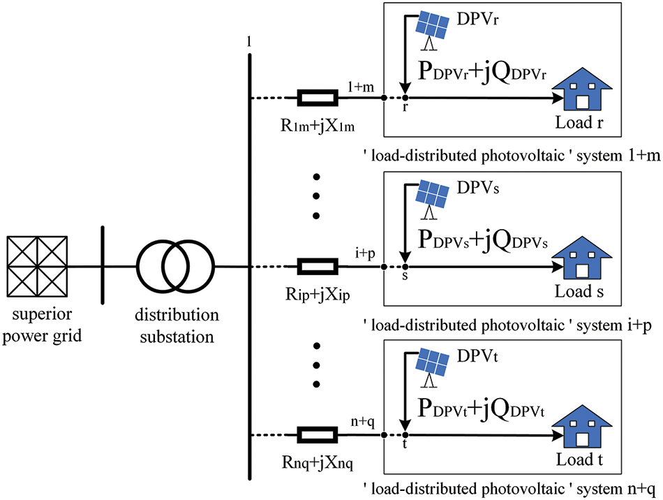
Figure 1: Schematic diagram of the distribution network with DPV

In Fig. 1, R is the line resistance, X is the line reactance, DPV is the distributed photovoltaics connected to the nearest load, and multiple sets of adjacent ‘load-distributed photovoltaics’ systems are together connected to the superior distribution network. The complex power injected by each DPV to the distribution network is PDPV + jQDPV, and the direction of load power flow is indicated in the diagram.

For a n-node distribution network, the power equation of any node i is

Pi−jQi=U∗i∑k=1nYikU⋅k(1)

where Pi is the active power injected by node i; Qi is the reactive power injected by node i; U∗i is the voltage conjugate phasor of node i; k is the remaining nodes of the distribution network except node i; U⋅k is the voltage phasor of node k; Yik is the admittance of branch i–k; j is the phase imaginary unit.

Eq. (1) reflects that when the structure and parameters of the distribution network are constant, the injection power of a node depends on the voltage of each node. Conversely, the voltage value U of any node i can be determined by the injection power of each node in the network, that is

Ui=f(P1,…,Pi,…,Pn;Q1,…,Qi,…,Qn)   i=1,…,n(2)

When a photovoltaic system is connected, the voltage values of any node i change as follows:

Uinew=Ui+ΔUik=fi(P1,…,Pk−PkPV,…,Pn;Q1,…,Qk+QkPV,…,Qn)i,k=1,…,n(3)

where Uinew is the voltage value of node i after connecting a new photovoltaic system to the network; ΔUik is the voltage increment of node i caused by photovoltaics connected to node k; PkPV is the active power injected into network by photovoltaics connected to node k; QkPV is the reactive power injected into network by photovoltaics connected to node k, which is positive when the power factor is lagging, and negative when the power factor is advanced; n is the total number of node in the distribution network.

It can be seen from Eq. (3) that the voltage increment of node i depends on the power injected into the distribution network by new grid-connected photovoltaics, that is, the voltage increment model of DPV grid-connected is

ΔUik=fiΔ(PkPV,QkPV)   i,k=1,…,n(4)

When continuously connecting DPVs to the r, s, t nodes in Fig. 1 in any order, the voltage increments ΔU1+m,r, ΔU1+m,s and ΔU1+m,t at the node 1 + m obtained by Eq. (4) are also arbitrary in the grid-connected process. In other words, connecting DPV to each node of the distribution network in turn in terms of different orders, the order of the voltage increment variation at the same node is different. The process of the voltage increment variation is random.

When large-scale DPV is connected to the distribution network, to effectively analyze its impact on the voltage of the distribution network, it is necessary to give an orderly grid-connected method to solve the disorder problem of the voltage variation.

3  Distributed Photovoltaics Orderly Grid-Connected Method

The orderly voltage impact analysis method is to reflect the orderliness of the node voltage change in distribution networks during a grid-connected process through a DPV grid-connected sequence, that is, the DPV orderly grid-connected method for voltage impact analysis.

3.1 Methods and Implementation Framework

In the process of voltage impact analysis, with DPV connected, the state of connecting photovoltaics to the distribution network (hereinafter referred to as the state) is changing. Compared with the previous state, the new grid-connected node in the current state is called the photovoltaics permitted grid-connected node. The photovoltaics permitted grid-connected node randomly selected in each state is recorded as Xm, and m is the number of states. Then the process of determining the photovoltaics permitted grid-connected node of the distribution network can be described as such event:

A={X1,X2,…,Xm}(5)

Event set A consists of m sub-events ‘determine Xm', and the sub-event set Bmis

Bm={Xm=dm}={dm=1,  lm,r−=0|r−=1,2,…,n−m+1}(6)

where dm is the node sequence number of the photovoltaics permitted grid-connected node in the state m, mark 1 at the node sequence number, indicating that it is the photovoltaics permitted grid-connected node in the current state; lm,r− is the r– node sequence number that the node is not connected to photovoltaics in the state m, which marked as 0.

To reflect voltage impact degree in an orderly method when photovoltaics are connected to different network nodes, it is necessary to highlight the impact of new grid-connected photovoltaics on the local node voltage as the principle. In other words, when determining the photovoltaics permitted grid-connected node in each state, it has to reflect its large voltage magnitude increase and the relatively small voltage magnitude increase of other nodes in the network. Then, in the process of photovoltaics grid-connected, the voltage incremental variation of the photovoltaics permitted grid-connected node reflects the orderliness of the voltage variation. In this sense, in the process of determining the photovoltaics permitted grid-connected nodes, Eq. (6) of any state is equivalent to Eqs. (7)–(9):

B={max(σ1),min(σ2)}(7)

σ1=g1(ΔUj),j∈NTN(8)

σ2=g2(∑r∈EΔUr)(9)

where σ1 is the measuring voltage increment index of the photovoltaics exploratory grid-connected node; σ2 is the measuring voltage increment index of other nodes in the network; ΔUj is the voltage increment of photovoltaics exploratory grid-connected node j; ΔUr is the voltage increment of the other node r; max and min are taking the maximum and minimum values; g1 and g2 are the corresponding function transformation rules; NTN is the set of photovoltaics exploratory grid-connected nodes; E is the set of other nodes in the network except the photovoltaics exploratory grid-connected node, specifically

E={r|r≠j,j∈NTN,r∈NPQ}(10)

where NPQ is the set of PQ nodes in the network.

The implementation framework of the DPV orderly grid-connected method proposed in this paper is shown in Fig. 2. In a certain state, by comprehensively measuring the index σ1 of each exploratory grid-connected node and the index σ2 of other nodes when the photovoltaics exploratory grid-connected node is given, the photovoltaics permitted grid-connected node is determined, and then the photovoltaics grid-connected state is continuously updated in the network to obtain the DPV grid-connected order that can reflect maximum node voltage increment variations. Compared with the previous state, the number of photovoltaics exploratory grid-connected nodes in the current state is reduced by one, and the number of photovoltaics permitted grid-connected nodes is increased by one, so the photovoltaics permitted grid-connected node in the last state is automatically determined.

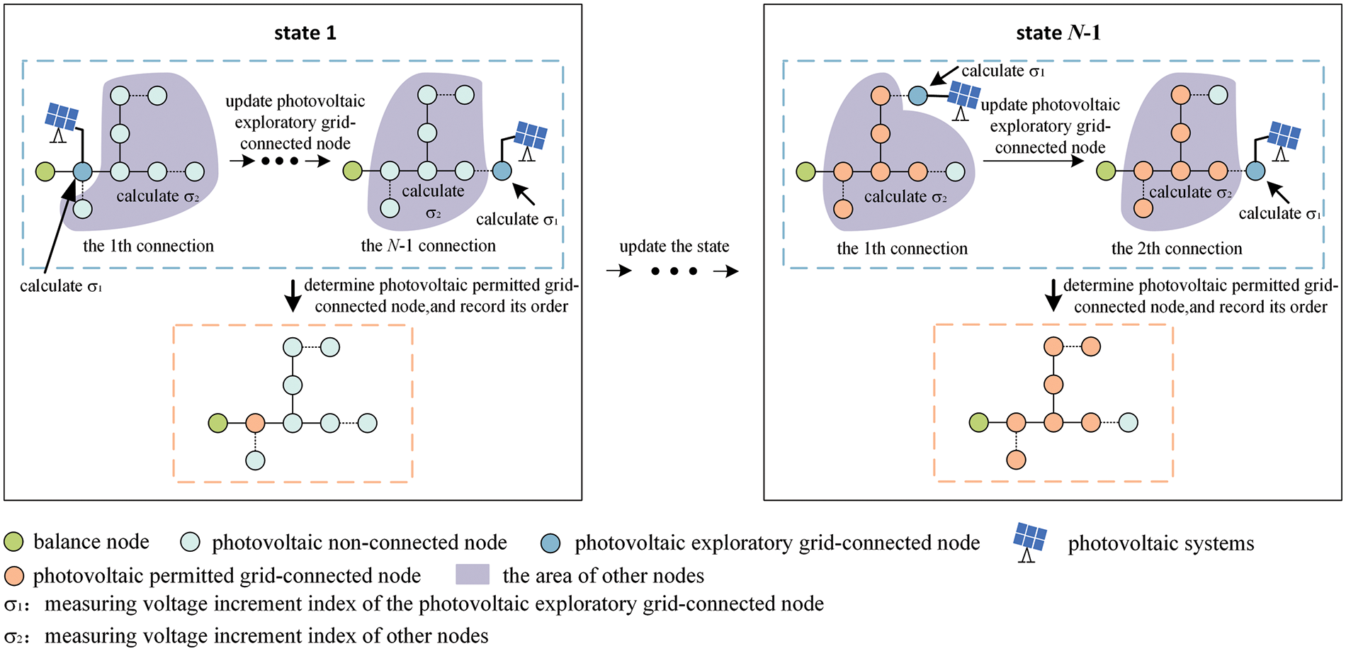
Figure 2: Method implementation framework

3.2 Photovoltaics Permitted Grid-Connected Node Determination Based on PGOD

In the stage of determining the photovoltaics permitted grid-connected node of each state, first of all, to effectively measure the voltage increment of the photovoltaics exploratory grid-connected node, index σ1 considers its response degree to the change of injected power. Firstly, the matrix form of the voltage sensitivity equation is given as shown in Eq. (11) [22], which reflects the coupling relationship between the node injection power and the node voltage.

[ΔδΔU]=[SδPSδQSUPSUQ][ΔPΔQ]=[∂δ∂P∂δ∂Q∂U∂P∂U∂Q][ΔPΔQ](11)

where Δδ is the node voltage phase angle change column vector; ΔU is the node voltage magnitude change column vector; ΔP is the node injected active power change column vector; ΔQ is the node injected reactive power change column vector; SδP reflects the change of node injected active powers impact on the change of voltage phase angles in the network; SUP reflects the change of active powers injected into PQ nodes impact on the change of voltage magnitudes in the network; SδQ reflects the change of reactive powers injected into PQ nodes impact on the change of voltage phase angles in the network. SUQ reflects the change of reactive powers injected into PQ nodes impact on the change of voltage magnitudes of PQ nodes.

It can be seen from Eq. (11) that a node voltage magnitude change of the PQ node has to respond to both active power and reactive power injections of each PQ node at the same time. To comprehensively characterize the sensitivity of the node voltage magnitude to both responses (only considering the value, ignoring its increase or decrease), the active weight coefficient WP and the reactive weight coefficient WQ are introduced, that is

WP=∑i∈NPQ∑k∈NPQ|∂U∂P|ik|∑i∈NPQ∑k∈NPQ|∂U∂P|ik|+∑i∈NPQ∑k∈NPQ|∂U∂Q|ik|(12)

WQ=∑i∈NPQ∑k∈NPQ|∂U∂Q|ik|∑i∈NPQ∑k∈NPQ|∂U∂P|ik|+∑i∈NPQ∑k∈NPQ|∂U∂Q|ik|(13)

where ∂U∂P|ik is the row i and column k element of SUP; ∂U∂Q|ik is the row i and column k element of SUQ.

The sensitivity of the node voltage magnitude to the change of node injection power is defined as VMS. Because only the VMS of the PQ node is considered, the SUP and SUQ are the same order square matrices. Combining the corresponding position elements in the two square matrices, the VMS vector S is obtained:

S={Sk|Sk=∑i=1N(WP∂U∂P|ik+WQ∂U∂Q|ik)}(14)

where N is the total number of the PQ node, i, k = 1,…, N; Sk is the k column element of the VMS vector. It needs to be stressed that elements of SUP and SUQ are added by column.

From Eqs. (8) and (14), it can be seen that the VMS value can reflect the voltage magnitude variation degree when different network nodes are connected to the same capacity photovoltaics. Therefore, VMS can be used as index σ1 to measure voltage increments of the photovoltaics exploratory grid-connected node.

Secondly, to effectively measure the voltage increment of other nodes in the network, index σ2 considers the acceptance of photovoltaics permitted grid-connected node of other nodes in the network due to their voltage changes, that is AoGCN.

The voltage magnitude relative variation Cr of the other node r in the network is

Cr=|Urnext_state−Urcurrent_state|Urcurrent_state(15)

where Urnext_state is the voltage magnitude of node r in the next state; Urcurrent_state is the voltage magnitude of node r in the current state.

After connecting DPV to the network at node j, the AoGCN value Aj is

Aj=∑r∈NPQr≠jlog0.5⁡(Cr)N−1(16)

From Eqs. (9), (15) and (16), it can be seen that the AoGCN value can reflect the voltage magnitude variation degree of other nodes in the network when the given exploratory grid-connected node is connected to photovoltaics, that is, the larger the Aj value, the smaller the voltage magnitude relative variation of the other node in the network, and the higher the acceptance of the current photovoltaics permitted grid-connected node. Therefore, AoGCN can be used as index σ2 to measure voltage increments of the other nodes in the network.

Further, to comprehensively reflect whether the exploratory grid-connected node j of any state can be used as the photovoltaics permitted grid-connected node through index σ1 and index σ2, a comprehensive index σ3 based on PGOD is constructed:

σ3=h1(σ1)+h2(σ2)(17)

where h1 and h2 are the transformation rules of index σ1 and index σ2.

Then, the PGOD value Oj of node j is

Oj=WjSSj+WjAAj(18)

where WjS is the weight coefficient of VMS when the photovoltaics is connected to node j; WjA is the weight coefficient of AoGCN when the photovoltaics is connected to node j; Sj is the VMS value of node j.

The S value of the photovoltaics exploratory grid-connected node j and the A value determined by other nodes in the network are all functions of the voltage increment ΔU. Then, WjS and WjA can be expressed as

WjS=ΔUjΔUj+∑r=1N−1ΔUrN−1(19)

WjA=∑r=1N−1ΔUrN−1ΔUj+∑r=1N−1ΔUrN−1(20)

where ΔUj is the voltage magnitude absolute variation of node j; ΔUr is the voltage magnitude absolute variation of node r.

From the above, the larger the S value is, the larger the index σ1 is, and the larger the voltage variation of the photovoltaics permitted grid-connected node is; the larger the A value is, the smaller the index σ2 is, the smaller the voltage variation of the other node in the network is, and the greater the acceptance of photovoltaics permitted grid-connected node is. Therefore, in one state, the photovoltaics permitted grid-connected node with the largest O value of index σ3 can comprehensively reflect the maximum impact of the new grid-connected photovoltaics on the network voltage by characterizing the S value of index σ1 and the A value of index σ2.

3.3 Photovoltaics Orderly Grid-Connected Process

Based on determining the photovoltaics permitted grid-connected node of a given state based on the PGOD, the photovoltaics grid-connected state is continuously updated in the network, and the photovoltaics orderly grid-connected model is obtained. The model is characterized by a directed row vector, as shown in Eq. (21).

D→={d1,…,dN|max{OmNS}=WdmSSdm+WdmAAdm,m=1,…,N}(21)

where OmNS is the set of the photovoltaics permitted grid-connected node in state m.

According to this model, the DPV grid-connected order of orderly voltage impact analysis can be obtained, which reflects two voltage variations:

1)   m is a constant value

At this time, there is a max {ONS} value at node dm, which reflects the maximum impact of the new grid-connected photovoltaics on node voltage in the current state.

2)   The m value is increasing

In this process, the node dm is continuously determined, and the max {ONS} value is continuously changed, which reflects the variation of the maximum node voltage increment in the network, and orderly reflects the impact of photovoltaics connected to different nodes on the voltage.

The implementation process of determining the DPV grid-connected order according to this model is shown in Fig. 3, where the initial state m = 0 is the state of no photovoltaics connected to the grid. It has to be noted that, in the process of DPV orderly grid-connected, the voltage impact should be analyzed at the same time.

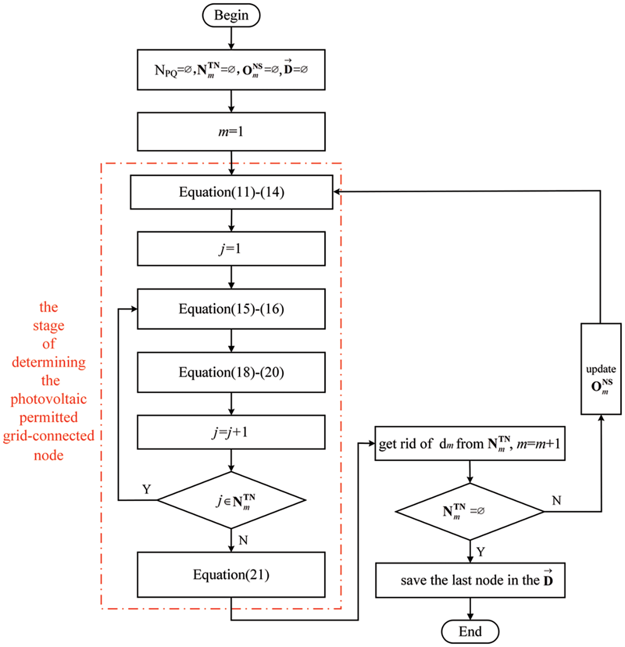
Figure 3: The process of getting the DPV grid-connected order

3.4 Grid-Connected Orderliness Evaluation Index

To illustrate whether the grid-connected order determined by the method proposed in this paper can analyze the voltage impact of large-scale DPV grid-connected in an orderly method, the grid-connected orderliness evaluation index is given in this section.

1)   Order coincidence degree

αm=arccos⁡(Ummax,f−Um−1max,f)2+(Ummax,s−Um−1max,s)2+2−(|Ummax,f−Um−1max,f|−|Ummax,s−Um−1max,s|)22(Ummax,f−Um−1max,f)2+1(Ummax,s−Um−1max,s)2+1m≠0,1(22)

where αm is the order coincidence degree of the photovoltaics permitted grid-connected node in state m; Ummax,s is the maximum voltage increment after photovoltaics are connected to the photovoltaics permitted grid-connected node in state m; Um−1max,s is the maximum voltage increment after photovoltaics are connected to the photovoltaics permitted grid-connected node in state m − 1; Ummax,f is the actual maximum voltage increment in state m; Um−1max,f is the actual maximum voltage increment in m − 1 state. In this paper, nodes with αm less than 1.00 × 10−4 are defined as orderly grid-connected nodes.

2)   Maximum voltage increment degree

β1=|U1max,s−U1max,f|U1max,f×100%(23)

where β1 is the maximum voltage increment degree of the photovoltaics single-connected state; U1max,s is the maximum voltage increment of the photovoltaics single-connected state in the order determined by Eq. (21); U1max,f is the actual maximum voltage increment of the photovoltaics single-connected state.

4  Case Analysis

4.1 Parameters Setting

To verify the effectiveness of the proposed method, a 97-node distribution network of a county in Northern China is used as the example system, and MATPOWER is used to calculate its power flow.

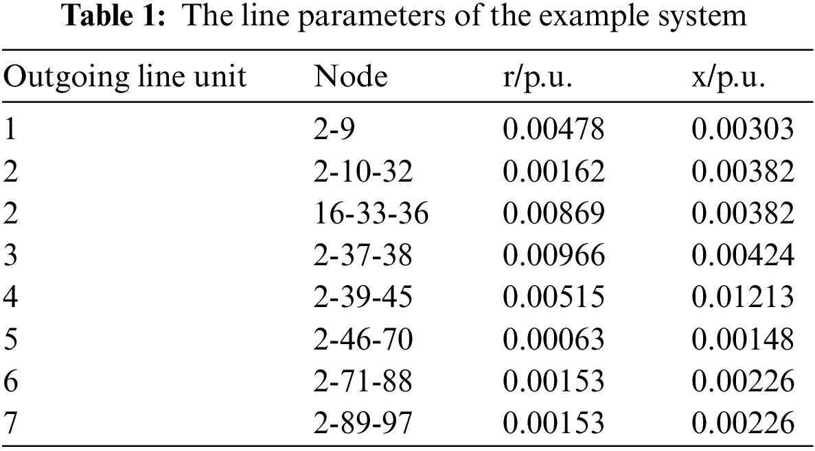
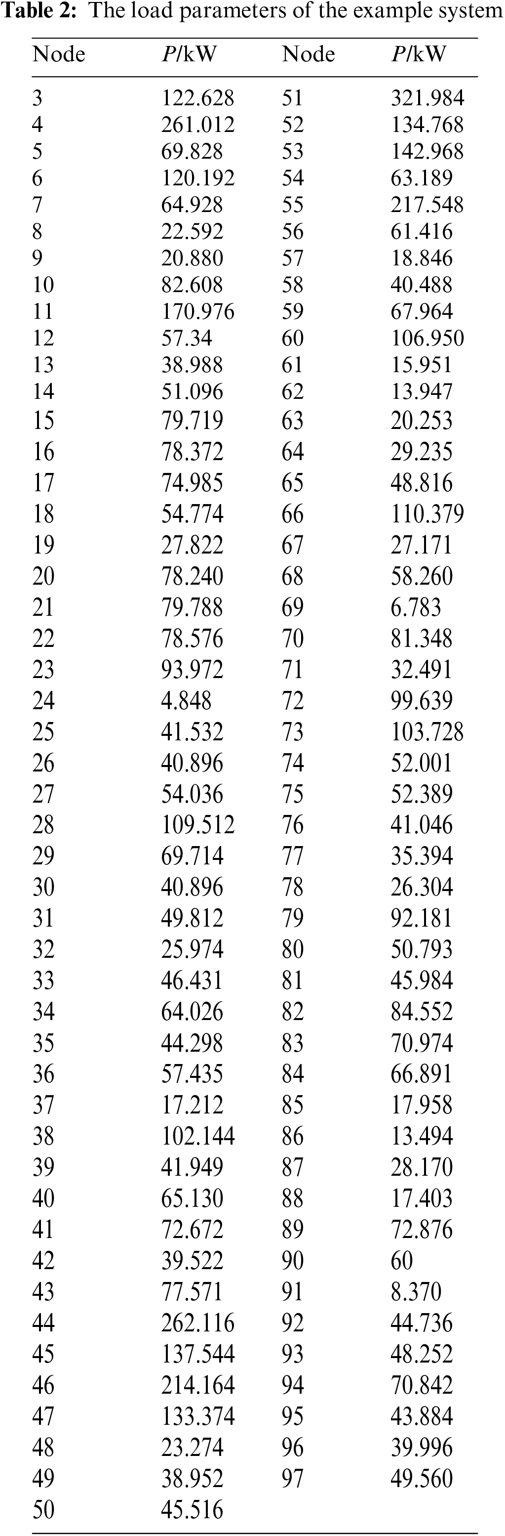
The structure of the example system is shown in Fig. 4. Line 1–2 is a 35/10 kV transformer with rated capacity of 20 MVA. The line parameters and load parameters are shown in Tables 1 and 2. The load is from 12:00 on the maximum load day of the example system, and its power factor is 0.95. Node 1 is a balanced node, node 2 is a PV node, and the other nodes in the system are PQ nodes. Therefore, a total of 95 nodes can be connected to DPV. Only active power injections of DPV are considered when connected to the grid, that is, the power factor of the photovoltaic system is 1.

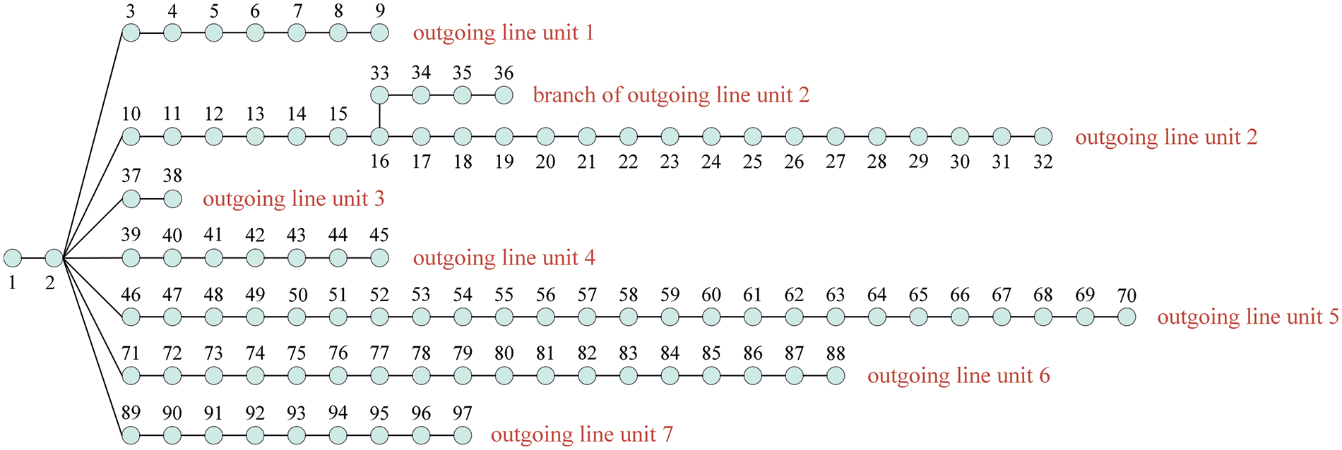
Figure 4: The structure diagram of the example system

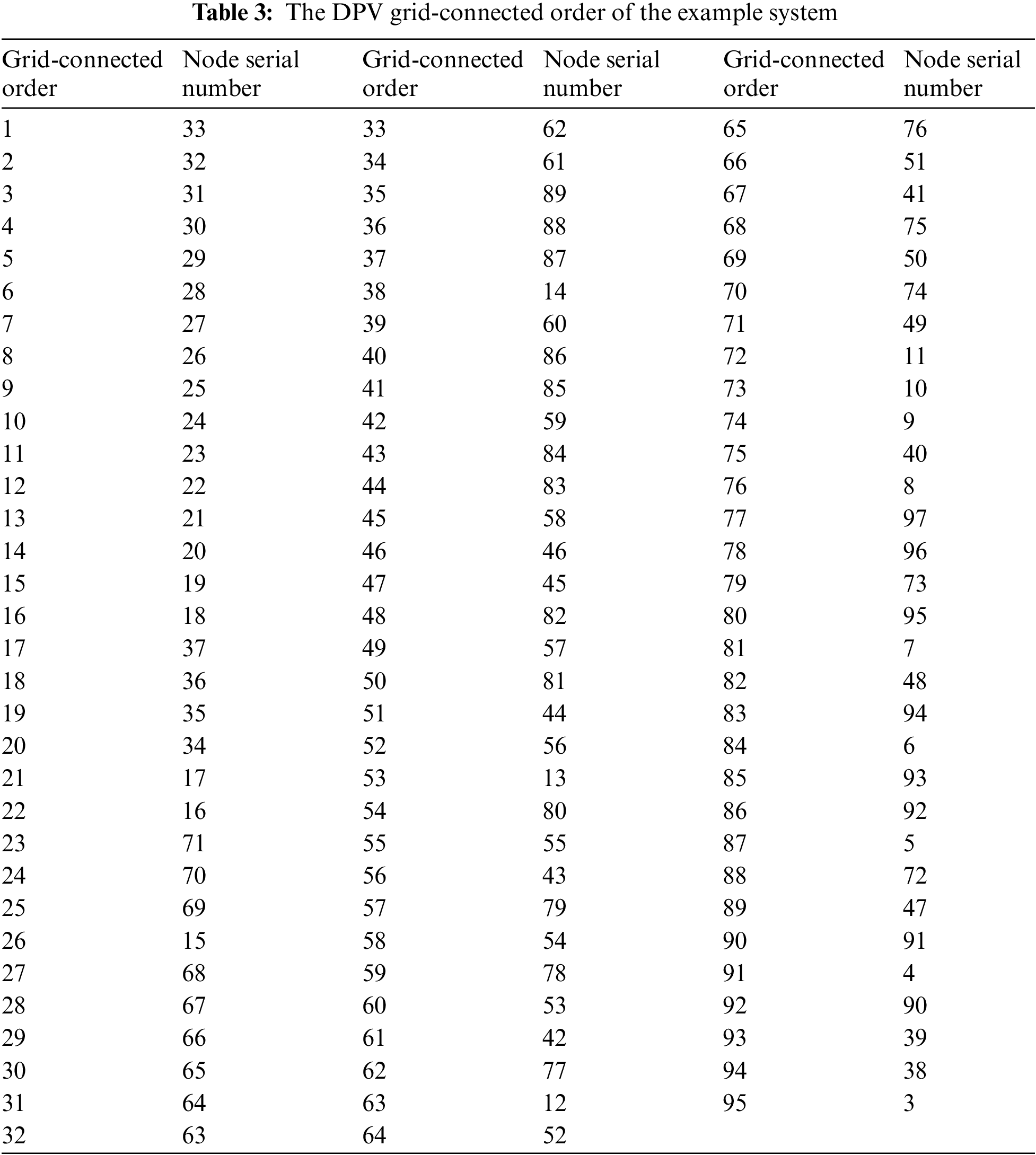
In the process of connecting DPV, as the degree of photovoltaics dispersion increases, the DPV capacity of each node is configured according to the proportion of the active load of the current grid-connected node to the total grid-connected node. The total active load capacity of the example system is 6.61 MW, and the total DPV grid-connected capacity is half of it, that is, 3.30 MW. The DPV grid-connected order is shown in Table 3.

4.2 Results Analysis

4.2.1 Verification of the Reasonability of Grid-Connected Order

In Fig. 5, the previous 94 maximum voltage dispersals of the example system are given after each exploratory grid-connected node is connected to DPV (with the increase of dispersal, the number of exploratory grid-connected nodes decreases), and the maximum voltage increment variation process of the example system is given after DPV are grid-connected in terms of the order as shown in Table 3.

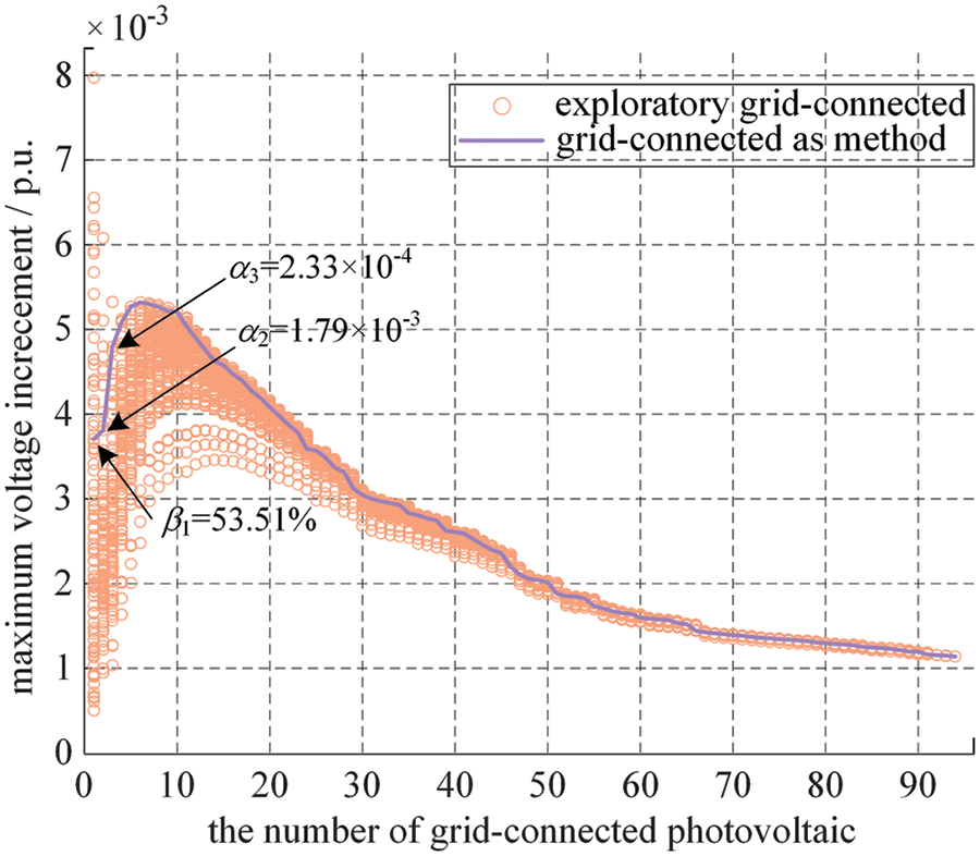
Figure 5: Maximum voltage increment variations with DPV connections in order

It can be seen from Fig. 5 that only under the previous 3 dispersals, β1 is 53.51%; α2 is 1.79 × 10−3 and α3 is 2.33 × 10−4, which are greater than 1.00 × 10−4, failing to effectively track the corresponding actual maximum voltage increment. With the increase of photovoltaics dispersal, the subsequent values α are less than 1.00 × 10−4, therefore, it can be considered that the determined photovoltaics grid-connected order can reflect the orderliness of large-scale DPV grid-connected and analyze voltage impact on the network. So, the DPV orderly grid-connected method is effective in this paper.

To validate that the proposed method can be well applied to radial distribution networks with different structures, a comparative example is added. In the comparative example, based on the original 97-node distribution network structure, the trunk line type part of outgoing unit 2 is only changed, its connection relationship changes to: “... -16-33-34-35-36-17...”, then the structure of the comparative example system is a completely radial topology.

The maximum voltage increment variations process of the comparative example system is shown in Fig. 6.

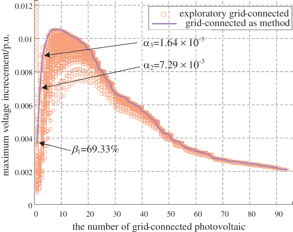
Figure 6: Maximum voltage increment variations in the comparative 97-node system

As shown in Figs. 5 and 6, actual voltage increments of the network are different due to the difference in topology, but maximum voltage increments can be traced when the number of grid-connected photovoltaic is greater than 3 according to the method proposed in this paper, which further demonstrates its effectiveness.

There are a large number of DPV grid-connected schemes in a given distribution network, which can be summarized as follows: 1) Under the premise of a certain DPV grid-connected capacity, there are many combinations of grid-connected locations in the network; 2) Under the premise of a certain grid-connected location, there are many combinations of DPV grid-connected capacity of each node. To reveal the main factors that voltage variations of each node are different in the distribution network and effectively analyze the impact of large-scale DPV connected on the voltage of the radial distribution network, the following cases are designed.

4.2.2 Voltage Impact Analysis under Different Dispersals and the Same DPV Capacity

In this case, the photovoltaics grid-connected capacity of each node is still configured according to the proportion of the active load of the current grid-connected node to the total grid-connected node, and the total DPV grid-connected capacity is 6.61 MW in the example system.

Fig. 7 shows the voltage magnitude distributions of each node (including node 1) under three different DPV grid-connected scenarios, which are the initial voltage magnitude distribution, the voltage magnitude distribution after the maximum PGOD node (node 33) of the initial network is connected to photovoltaics, and the voltage magnitude distribution after 95 joinable nodes are all connected to photovoltaics.

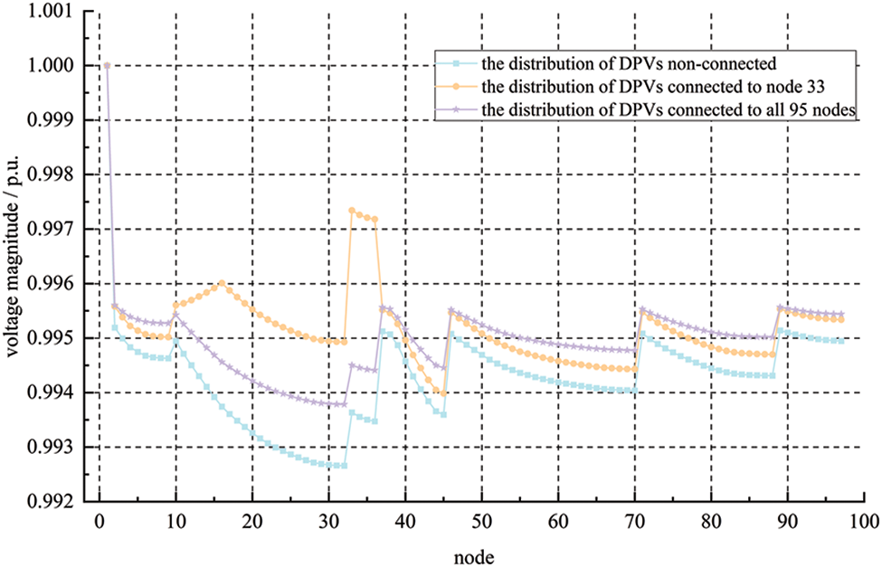
Figure 7: Voltage magnitude distributions under different DPV grid-connected schemes

From Fig. 7, it can be seen that, first, after all photovoltaics are connected to node 33, the voltage magnitude of node 33 rises most obviously. Then, after gradually increasing photovoltaics dispersals, the fluctuation degree of the node voltage magnitude distribution in the network gradually decreases. Finally, until the photovoltaics dispersal is maximized, voltage magnitudes of node 3–9 and node 37–97 increase slightly.

From the two aspects of VMS and AoGCN: 1) Voltage magnitudes of node 3–9 and node 37–97 are more responsive to their injection power changes; 2) When photovoltaics is connected to node 33 alone, node 3–9 and node 37–97 are less affected by it, and their acceptances of node 33 is high, that is, their voltage magnitude increment contributes the most to A33 value; 3) Combined with Fig. 4, it can be seen that compared with the branch of node 33, branches of node 3–9 and node 37–97 belong to different outgoing line units, and the electrical distance from node 33 is far, so they are less affected by the photovoltaics connected to node 33, that is, electrical distance determines the A value. In summary, due to the limitation of the node’s own VMS and electrical distance between nodes, the node voltage magnitude of the example system varies differently.

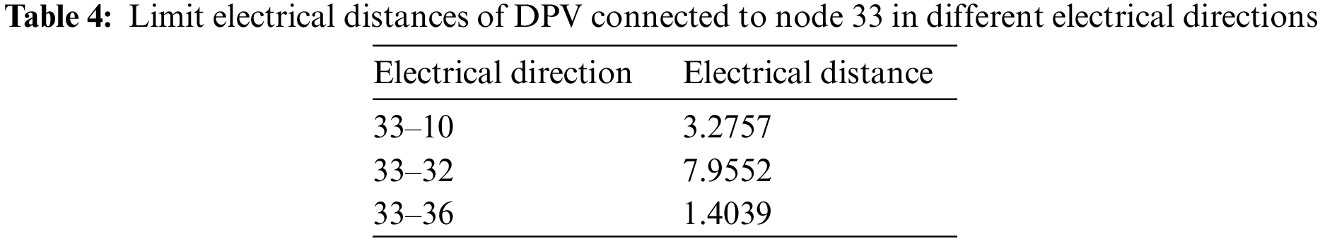
Based on the above analysis, the area where the outgoing line unit 2 is located is called the main action area of node 33 photovoltaics, and the remaining area is called the secondary main action area of node 33 photovoltaics. Fig. 8 shows the division of the photovoltaics action area of node 33 based on VMS and electrical distance. The electrical distance in different directions is characterized by the total reactance of the branch, as shown in Table 4. In Fig. 8, the shadow area is the main action area of photovoltaics connected to node 33, voltage magnitude variations of this area mainly depend on the photovoltaics connected to node 33, and the main action area with an electrical distance less than 1.4039 entirely depends on the electrical distance from node 33. The non-shadow area is the secondary main action area of photovoltaics connected to node 33, voltage magnitudes in this area are more impacted by the photovoltaics connected to the own location. And the attributes of the two area boundaries are the same as the shadow area.

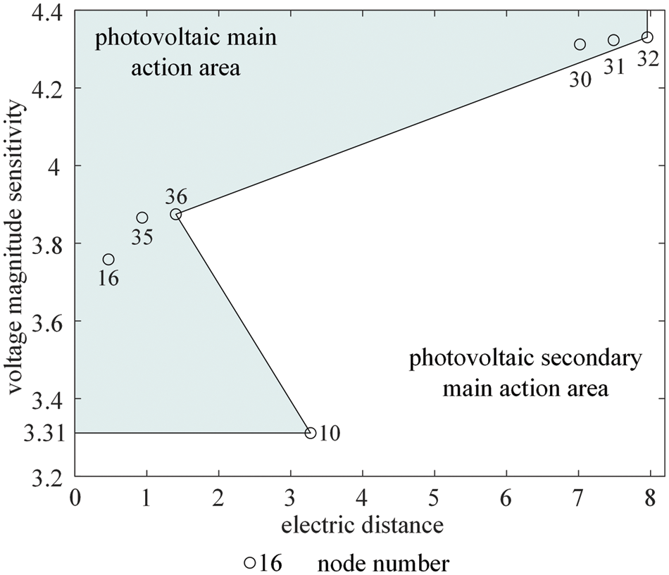
Figure 8: Division of the DPV action area

Further, the distribution of photovoltaics main action areas in the example system is given in Fig. 9, based on its actual spatial distribution map of the outgoing line unit. It can be seen from Fig. 9 that each outgoing line unit of the distribution substation (the total number is 7) is a photovoltaics main action area, and in this area, the voltage magnitudes are mainly impacted by photovoltaics grid-connected. Although the spatial geographical distance between the outgoing line unit 4 and the outgoing line unit 5 is relatively close, they still belong to different photovoltaics main action areas, this is because voltage magnitudes of the other outgoing line unit are less affected and AoGCN is higher when photovoltaics is newly connected to a certain outgoing line unit due to the limitation of electrical distance. On each outgoing line unit, VMS determines different voltage magnitude variations of each node.

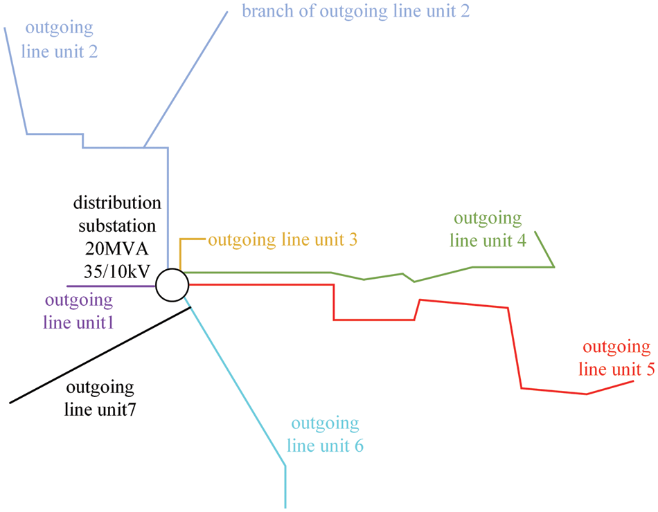
Figure 9: The distribution diagram of photovoltaics main action areas in the example system

Next, we will explore the impact degree of different positions on voltage. In this paper, the dual voltage impact degree of the new grid-connected node and the other node in the network under each state from photovoltaics is comprehensively considered. This impact degree is described by PGOD value. Therefore, the distribution of PGOD under each state is given in Fig. 10, to further explain the impact degree of different photovoltaics grid-connected locations on voltage.

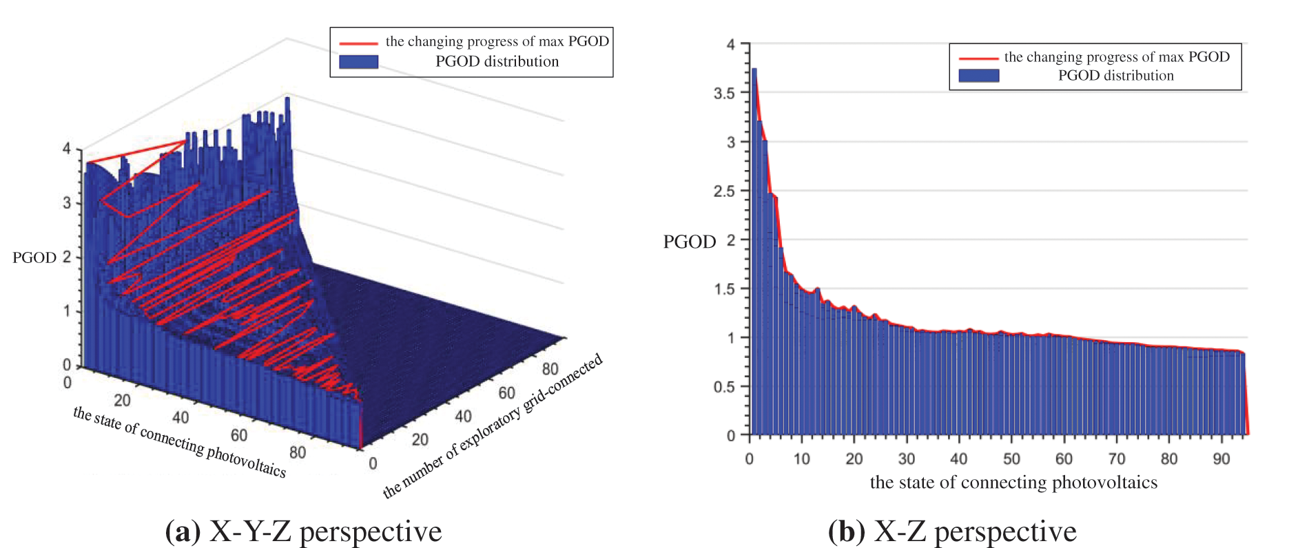
Figure 10: The distribution of PGOD in the grid-connected process

To more intuitively reflect the change process of the PGOD value in Fig. 10a, the X–Z perspective is given in Fig. 10b. It can be seen that PGOD values of each state gradually decrease, with the gradual increase of the photovoltaics location, which means that the increment of voltage magnitude gradually decreases in the network. Therefore, the more photovoltaics locations, the lower the impact degree on node voltage. The impact degree of photovoltaics connected to each node on voltage gradually decreases along the determined descending grid-connected order. It can be seen from Fig. 10b that the impact degree on the voltage of the photovoltaics full connection is 77.72% lower than that of the photovoltaics single connection. The reason for the above simulation results is that the more photovoltaics grid-connected nodes, the more photovoltaics that act together on the increment of voltage magnitude, and the less contribution of each node photovoltaics to the increment of voltage magnitude.

4.2.3 Voltage Impact Analysis under Different DPV Capacity and the Same Dispersals

In this case, scenarios of only node 33 connected to DPV and 95 joinable nodes all connected to DPV are selected for analysis. The DPV capacity variations of the given node are characterized by photovoltaics penetration rate, which ranges from 0% to 100%. The total active load capacity of the example system is 6.61 MW. In this paper, photovoltaics penetration rate Pe is defined as

Pe=PPVPload_PQ×100%(24)

where PPV is the total DPV grid-connected capacity; Pload_PQ is the total active load value of the PQ node.

Firstly, the scenario of only node 33 connected to DPV with different capacity is analyzed. In Fig. 11, the voltage magnitude distribution is given when photovoltaics penetration rates are 0%, 20% (the total grid-connected capacity of DPV is 1.32 MW), and 90% (the total grid-connected capacity of DPV is 5.95 MW).

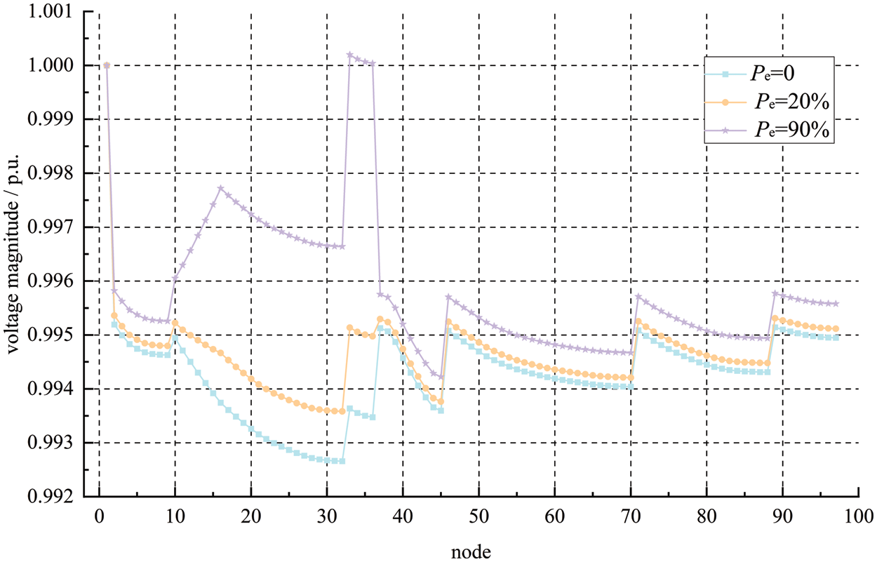
Figure 11: Voltage distributions of different capacity with DPV connected to node 33

It can be seen from Fig. 11 that, as the photovoltaics grid-connected capacity of node 33 increases, all the voltage magnitudes of node 3–97 increase, and the voltage magnitude fluctuates greatly in the example system. Since the electrical distance of the photovoltaics connected to node 33 effect on itself is 0 and the VMS of node 33 is largest, its voltage magnitude rises most obviously. When the total DPV grid-connected capacity exceeds 5.95 MW, the maximum voltage magnitude of the example system will be transferred from the balance node (node 1) to the maximum PGOD node (node 33), and then the voltage magnitudes of the other node will gradually exceed node 1.

The variation of the minimum node voltage magnitude in the above process is shown in Fig. 12. When photovoltaics is not connected, the minimum voltage magnitude of the example system appears at node 32. When the total DPV grid-connected capacity exceeds 1.32 MW, the minimum node voltage magnitude of the example system begins to transfer to other nodes.

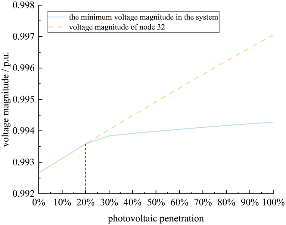
Figure 12: The change of minimum voltage in the system under different capacity with DPV connected to node 33

Secondly, 95 joinable nodes all connected to different DPV capacity scenarios are analyzed. In Fig. 13, the voltage magnitude distribution is given when photovoltaics penetration rates are 0, 50% (the total grid-connected capacity of DPV is 3.30 MW), and 100%.

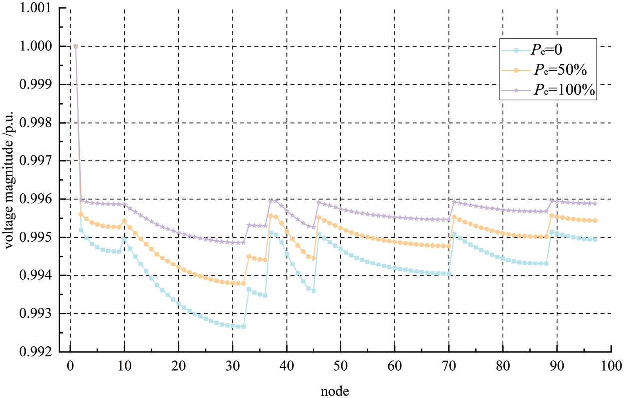
Figure 13: Voltage distributions of different capacity with DPV connected to all nodes

It can be seen from Fig. 13 that, in these scenarios, the voltage magnitude fluctuation range is small in the example system. In this process, the maximum voltage magnitude is always constant at the balance node (node 1), and the minimum voltage magnitude is always constant at node 32.

Next, we discuss the impact degree of photovoltaics capacity on voltage in two scenarios of photovoltaics single-connected and full-connected, as shown in Figs. 14 and 15. Based on the simulation results of Fig. 14, it can be seen that: (1) the node voltage magnitude increases linearly with photovoltaics grid-connected capacity, which is because the active power injected by the photovoltaic system into the distribution network increases; (2) as grid-connected capacity increases, the voltage magnitude of the new grid-connected photovoltaics node increases more than the average voltage magnitude of the other node in the network. With the increase of the photovoltaics grid-connected node, the voltage magnitude of the new grid-connected photovoltaics node gradually decreases, tending to the average voltage magnitude of the other node in the network. It can be seen from Fig. 15 that with the increase of photovoltaics grid-connected nodes, the voltage magnitude increment of the connected photovoltaics node gradually decreases with the increase of grid-connected capacity, which is reduced by 0.50%. Therefore, grid-connected DPV should have a certain dispersal degree.

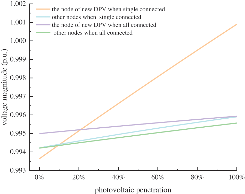
Figure 14: Voltage magnitude variations with photovoltaics capacity increasing

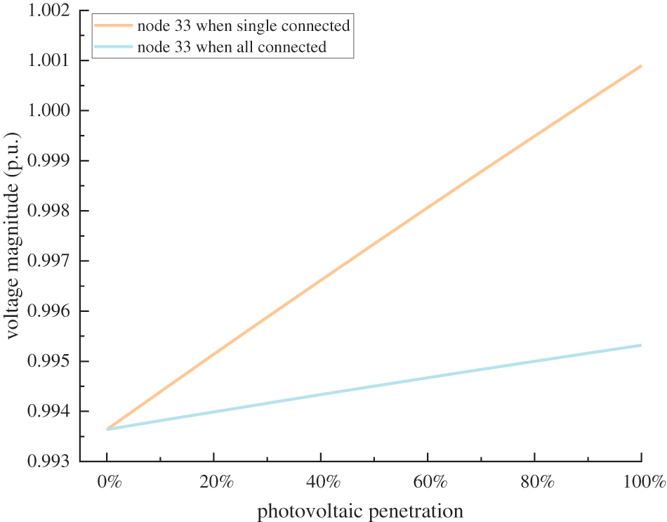
Figure 15: Voltage magnitude variations of node 33 with photovoltaics capacity increasing

In summary, the more photovoltaics grid-connected capacity, the higher its impact on voltage, but with the locations (grid-connected nodes) increase, this impact degree gradually decreases.

5  Conclusion

Under the background of a large-scale DPV connected to county distribution networks, to reflect the impact of photovoltaics connected to different nodes on voltage in an orderly method, and carry out voltage impact analysis at the same time, this paper presents a photovoltaics orderly grid-connected method based on PGOD. The effectiveness of this method is verified by an example simulation. The conclusions are as follows:

1)    In the process of DPV grid-connected according to the order determined by the method in this paper, the actual maximum voltage increment under each dispersal can be effectively tracked, and the impact of photovoltaics connected to different nodes on voltage can be reflected in sequence.

2)    The variation of node voltage magnitude in the radial distribution network is subject to the dual constraints of voltage magnitude sensitivity and electrical distance. Based on this, the single-node grid-connected photovoltaics form a main action area in its outgoing line unit, and other outgoing line units are the secondary main action area.

3)    Under the premise of a certain total capacity of DPV, the voltage magnitude of each node in the photovoltaics main action area decreases with a gradual increase of photovoltaics dispersal. In the photovoltaics secondary main action area, the voltage magnitude of each node will increase in this process due to the connection to itself.

4)    Under the premise of a certain location of DPV, the grid-connected capacity is gradually increased, and the voltage magnitude of each node is increased. When a single node is connected to photovoltaics, the voltage magnitude fluctuates greatly, and when the photovoltaics penetration rate exceeds 20%, the location where the minimum voltage is located transfers to other nodes; when the photovoltaics penetration rate exceeds 90%, the location where the maximum voltage is located is transferred. When all joinable nodes are connected to photovoltaics, the fluctuation of voltage magnitude is small. Within 100% of the photovoltaics penetration rate, the location where the maximum voltage is located will not transfer.

In summary, when planning DPV constructions, it should be noted that grid-connected DPVs should have a certain dispersal degree. The nodes with the lowest rank (smallest impact degree on voltage) should be given priority when making a reasonable decision on DPV connection nodes based on the VMS value of each node and the electrical distance between nodes. Based on the construction idea of this method, an effective method can be established to analyze the impact of DPV connections on line load rate for the distribution network construction. Further, strategies can be designed to determine the comprehensive impact of grid-connected nodes on the network in the field such as photovoltaics configuration research, and then the distribution of distributed power sources is optimized. We will carry out further research based on the above ideas in the future.

Acknowledgement: We would like to thank all the authors for their guidance and help on this article.

Funding Statement: This work is supported by North China Electric Power Research Institute’s Self-Funded Science and Technology Project “Research on Distributed Energy Storage Optimal Configuration and Operation Control Technology for Photovoltaic Promotion in the Entire County” (KJZ2022049).

Author Contributions: Kunqi Gao: writing the original draft; Cuiping Li, Junhui Li and Xingxu Zhu: writing–review & editing, supervision; Can Chen, Xiaoxiao Wang and Yinchi Shao: writing–review & editing, co-supervision. All authors reviewed the results and approved the final version of the manuscript.

Availability of Data and Materials: Data will be made available on request.

Ethics Approval: Not applicable.

Conflicts of Interest: The authors declare that they have no conflicts of interest to report regarding the present study.

References

1. S. C. Zhou, Y. F. Li, C. W. Jiang, Z. Xiong, J. H. Zhang and L. L. Wang, “Enhancing the resilience of the power system to accommodate the construction of the new power system: Key technologies and challenges,” Front. Energy Res., vol. 11, pp. 76, Sep. 2023. doi: 10.3389/fenrg.2023.1256850. [Google Scholar] [CrossRef]

2. B. Yang, Y. L. Li, Y. X. Ren, Y. X. Chen, X. S. Zhang and J. B. Wang, “Assessment on fault diagnosis and state evaluation of new power grid: A review,” Energ. Eng., vol. 120, no. 6, pp. 1287–1293, Apr. 2023. doi: 10.32604/ee.2023.027801. [Google Scholar] [CrossRef]

3. Z. Li, W. B. Wang, S. F. Han, and L. J. Lin, “Voltage adaptability of distributed photovoltaic access to a distribution network considering reactive power support,” (in Chinese), Power Syst. Protect. Control, vol. 50, no. 11, pp. 32–41, Jun. 2022. doi: 10.19783/j.cnki.pspc.211781. [Google Scholar] [CrossRef]

4. T. Y. Yao, Y. Li, X. B. Qiao, Y. Han, S. M. Jiao and Y. J. Cao, “Hosting capacity optimization of distributed photovoltaic in distribution network considering security boundary and coordinate configuration of SOP,” (in Chinese), Elect. Pow. Automat. Equipment, vol. 42, no. 4, pp. 63–70, Apr. 2022. doi: 10.16081/j.epae.202201024. [Google Scholar] [CrossRef]

5. Y. M. Ding, R. X. Cui, Q. M. Dai, H. J. Wang, Y. X. Cheng and W. Jia, “Lower voltage riding through control strategy for rural area distributed photovoltaic power generation system,” in 2023 8th ACPEE, Tianjin, China, 2023, pp. 483–487. [Google Scholar]

6. T. Aziz and N. Ketjoy, “PV penetration limits in low voltage networks and voltage variations,” IEEE Access, vol. 5, pp. 16784–16792, Aug. 2017. doi: 10.1109/ACCESS.2017.2747086. [Google Scholar] [CrossRef]

7. R. G. Suryavanshi and I. Korachagaon, “A review on power quality issues due to high penetration level of solar generated power on the grid,” in Proc. IEEE 2nd Int. Conf. Power Embedded Drive Control, 2019, pp. 464–467. [Google Scholar]

8. B. Y. Tan and L. A. Chen, “Research on the influence of distributed photovoltaic grid connection on voltage fluctuation,” in 2022 Power Syst. Green Energy Conf. (PSGEC), Shanghai, China, 2022, pp. 267–271. [Google Scholar]

9. D. Chathurangi, U. Jayatunga, S. Perera, and A. Agalgaonkar, “Evaluation of maximum solar PV penetration: Deterministic approach for over voltage curtailments,” in Proc. IEEE PES Innov. Smart Grid Technol. (ISGT-Europe), Bucharest, Romania, 2019, pp. 1–5. [Google Scholar]

10. K. Ndirangu, H. D. Tafti, J. E. Fletcher, and G. Konstantinou, “Impact of grid voltage and grid-supporting functions on efficiency of single-phase photovoltaic inverters,” IEEE J. Photovolt., vol. 12, no. 1, pp. 421–428, Jan. 2022. doi: 10.1109/JPHOTOV.2021.3127993. [Google Scholar] [CrossRef]

11. G. Magdy, M. Metwally, A. A. Elbaset, and E. Zaki, “Performance assessment of a real pv system connected to a low-voltage grid,” Energy Eng., vol. 121, no. 1, pp. 13–26, Sep. 2023. doi: 10.32604/ee.2023.043562. [Google Scholar] [CrossRef]

12. Y. Liu, W. P. Qin, L. Wang, X. Q. Han, P. Wang and Y. P. Xiang, “Voltage control strategy of PV grid-connected inverter in low voltage distribution network with reduction amount of light discarded,” (in Chinese), Acta Energiae Solaris Sinica, vol. 41, no. 8, pp. 151–159, Aug. 2020. doi: 10.19912/j.0254-0096.2020.08.021. [Google Scholar] [CrossRef]

13. S. Rahman et al., “Analysis of power grid voltage stability with high penetration of solar PV systems,” IEEE Trans. Ind. Appl., vol. 57, no. 3, pp. 2245–2257, May–Jun. 2021. doi: 10.1109/TIA.2021.3066326. [Google Scholar] [CrossRef]

14. L. F. León, M. Martinez, L. J. Ontiveros, and P. E. Mercado, “Devices and control strategies for voltage regulation under influence of photovoltaic distributed generation. A review,” IEEE Lat. Am. Trans., vol. 20, no. 5, pp. 731–745, May 2022. doi: 10.1109/TLA.2022.9693557. [Google Scholar] [CrossRef]

15. M. R. Jafari, M. Parniani, and M. H. Ravanji, “Decentralized control of OLTC and PV inverters for voltage regulation in radial distribution networks with high PV penetration,” IEEE Trans. Power Deliv., vol. 37, no. 6, pp. 4827–4837, Dec. 2022. doi: 10.1109/TPWRD.2022.3160375. [Google Scholar] [CrossRef]

16. W. B. Zou, S. Han, N. Rong, and S. W. Chen, “Voltage control strategy for a PV inverter based on distributed consensus collaboration,” (in Chinese), Pow. Syst. Protect. Control, vol. 52, no. 1, pp. 166–173, Jan. 2024. doi: 10.19783/j.cnki.pspc.230648. [Google Scholar] [CrossRef]

17. Z. W. Cui, X. W. Li, D. Y. Zhu, X. H. Tan, and Y. G.Tao, “Study on steady-state voltage distribution of medium voltage distribution network considering high proportion distributed photovoltaic access,” in 2022 7th ICPRE, Shanghai, China, 2022, pp. 376–381. [Google Scholar]

18. A. M. M. Nour, A. A. Helal, M. M. El-Saadawi, and A. Y. Hatata, “Voltage violation in four-wire distribution networks integrated with rooftop PV systems,” IET Renew. Power Gener., vol. 14, no. 13, pp. 2395–2405, Oct. 2020. doi: 10.1049/iet-rpg.2020.0174. [Google Scholar] [CrossRef]

19. Y. Y. Shi, L. Ye, Z. Li, P. Lu, X. J. Chu and W. Z. Zhong, “Distributed photovoltaic power stations modeling and analysis of influence on voltage,” in 2022 IEEE/IAS Ind. Commer. Power Syst. Asia (I&CPS Asia), Shanghai, China, 2022, pp. 1314–1319. [Google Scholar]

20. Y. Chen, D. C. Liu, J. Wu, W. Chen, and Y. T. Xu, “Research on influence of distributed photovoltaic generation on voltage fluctuations in distribution network,” (in Chinese), Elect. Measurm. & Instrument., vol. 55, no. 14, pp. 27–32, Jul. 2018. [Google Scholar]

21. F. Jin et al., “Uncertainty analysis of DG hosting capacity in distribution network based on voltage sensitivity,” (in Chinese), Elect. Pow. Automat. Equip., vol. 42, no. 7, pp. 183–189, Jul. 2022. doi: 10.16081/j.epae.202204076. [Google Scholar] [CrossRef]

22. F. Ruiz-Tipán, C. Barrera-Singaña, and A. Valenzuela, “Reactive power compensation using power flow sensitivity analysis and QV curves,” in 2020 IEEE ANDESCON, Quito, Ecuador, 2020, pp. 1–6. [Google Scholar]