Multi-Branch Fault Line Location Method Based on Time Difference Matrix Fitting

1  Introduction

With the gradual increase in urbanization and city scale, the demand for electricity in modern society is also rising. As more loads are connected to the distribution network, distribution lines with multiple branches serve the purpose of providing multiple power supplies to cater to the increasing number of loads [1]. To enhance the stability, security, and efficiency of the power supply service in the grid, it is crucial to promptly and accurately locate the fault point when there is a failure in the multi-branch control line. The fault-traveling wave positioning time window is short, which means it has a fast response speed. It is not affected by factors such as neutral grounding mode, system parameters, and line asymmetry. As a result, it is highly favored by scholars both domestically and internationally [2]. The fault-traveling wave location can be divided into single-ended and double-ended locations. The single-ended location is determined by the time it takes for the traveling wave to travel back and forth once, multiplied by its velocity [3]. Marking the traveling wave head becomes challenging due to the influence of refraction and reflection caused by wave impedance discontinuity [4]. The reliability of single-ended traveling wave positioning theory is greatly reduced in distribution networks with multiple multi-branch lines, making it unsuitable for engineering applications [5]. The double-ended traveling wave location is achieved by measuring the time difference it takes for the original traveling wave to reach both ends of the line [6]. This method is based on a simple principle: knowing the arrival time of the original traveling wave head. It does not involve considering the refraction and reflection of wave impedance discontinuity points [7]. The fault location results are reliable and suitable for multi-branch distribution networks with wave impedance discontinuity [8].

1.1 Related Research Works

The distribution network has a complex topology, with each mainline containing numerous branches. Typically, traveling wave detection devices are installed at the end of the line rather than at the end of each branch. As a result, directly applying the double-ended traveling wave positioning method to multi-branch distribution networks is challenging [9]. The main methods for locating faults in multi-branch systems are the injection method and the traveling wave method. In recent years, scholars have extensively studied the application of traveling waves in multi-branch distribution networks. In reference [10], the largest of the two-end ranges is chosen for direct ranging. However, this means that when there are changes in line length or distribution network topology, it becomes impossible to detect fault branches. As a result, multi-branch fault line ranging fails. A fault location theory for multi-branch transmission lines based on a double-ended traveling wave was proposed, considering the influence of line parameters on distance measurement. This theory builds upon reference [11], which explores the relationship between the length of multi-branch lines and the location of fault points as described in reference [10]. The fault location is solved by combining the fault branch determination and the fault location algorithm. However, this method only considers the preset traveling wave velocity and does not take into account how inaccuracies in wave velocity can affect ranging accuracy. When the line parameters change, errors may occur between the calculated traveling wave velocity based on these parameters and the actual wave velocity. This method can be used to determine faults in multi-branch lines, but it does not guarantee accuracy for fault branches. The literature mentioned above mostly focuses on T-branch lines when discussing traveling wave fault location methods for multi-branch lines. However, these methods do not apply to lines with more than three branches. Despite this limitation, they still hold practical value in real-world applications. In reference [12], the Teager energy operator was proposed to extract the Intrinsic Mode Function (IMF) and calibrate the original traveling wave head of multi-branch lines. A matrix is formed at the arrival time of the original traveling wave to identify the fault branch. This method can be applied to circuits with multiple branches. Reference [13] simplified multi-branch fault lines into single-branch fault lines based on the findings of reference [12]. However, every element in the n-order fault matrix established by reference [13] needs to be corrected, which makes its calculation process more complicated. In reference [14], The current unbalance is defined based on the node where the fault branch is located. The fault location algorithm, as described in reference [14], converts into a unary quadratic solution. Additionally, reference [15] took into account the influence of distributed capacitor current and latent power supply current. However, this method relies on the action of relay protection devices. If a relay protection device has a blind spot in its action, it can lead to misjudgment and impact the accuracy of locating multi-branch faults.

Reference [16] proposed a model that is based on RFI state constraints. This model eliminates the restriction that all sources must have multiple faults on different paths, and it also improves the robustness of piece-based positioning. In reference [17], the machine learning method was used to analyze the depth features of steady and transient signals. Unlike traditional methods that require signal generators, this approach relies on shallow machine learning as a feature research model. However, these models cannot effectively extract fault features, resulting in some loss of important information. The method described in reference [18] is not effective for practical applications due to the small harmonic component, which cannot accurately describe the transient electrical characteristics of the system. In contrast, reference [19] improved positioning efficiency and accuracy by combining the genetic algorithm and particle swarm optimization algorithm using the minimum collision set criterion. References [16–19] all relied on self-modeling for section positioning or improving positioning accuracy. However, these methods face challenges such as difficulty in collecting fault samples, significant discrepancies between simulation and real-world scenarios, and limited practicality.

1.2 Research Contribution

Based on the analysis above, this paper proposes a new method for locating multi-branch faults by fitting the time difference matrix. The complex problem of locating faults in multi-branch lines is simplified by transforming it into a double-ended fault location problem. Additionally, the multi-branch lines are decomposed into mainlines that only consist of simple branches, such as T-branches or three-branches. The fault original traveling wave head in the fault line and non-fault line have different characteristics. To analyze this, we establish the decomposed baseline time difference matrix S and the fault time difference matrix G of the mainline endpoints. We then deeply analyze the time difference variation before and after a fault occurs on both lines. Additionally, we identify any changes in the elements of these matrices before and after a fault occurs. To minimize the impact of wave velocity on line parameters, we determine the wave velocity based on the arrival time of the original fault-traveling wave along the shortest path. This allows us to modify the parameters in matrices S and G. The least square method is used to fit the data of the row vector elements in matrices S and G. This helps determine the best first function match between the two-row vectors, which then determines the fault branch segment. This method is suitable for multi-branch circuits, improving the algorithm’s practicality. The proposed method has been verified for accuracy and reliability through theoretical analysis and simulation.

2  Time Difference Matrix Construction

2.1 Multi-Component Control Grid Line Decomposition

Fig. 1 depicts the network structure topology of a 10 kV distribution network. The length unit for each branch line is a meter, although this detail is not shown in the figure.

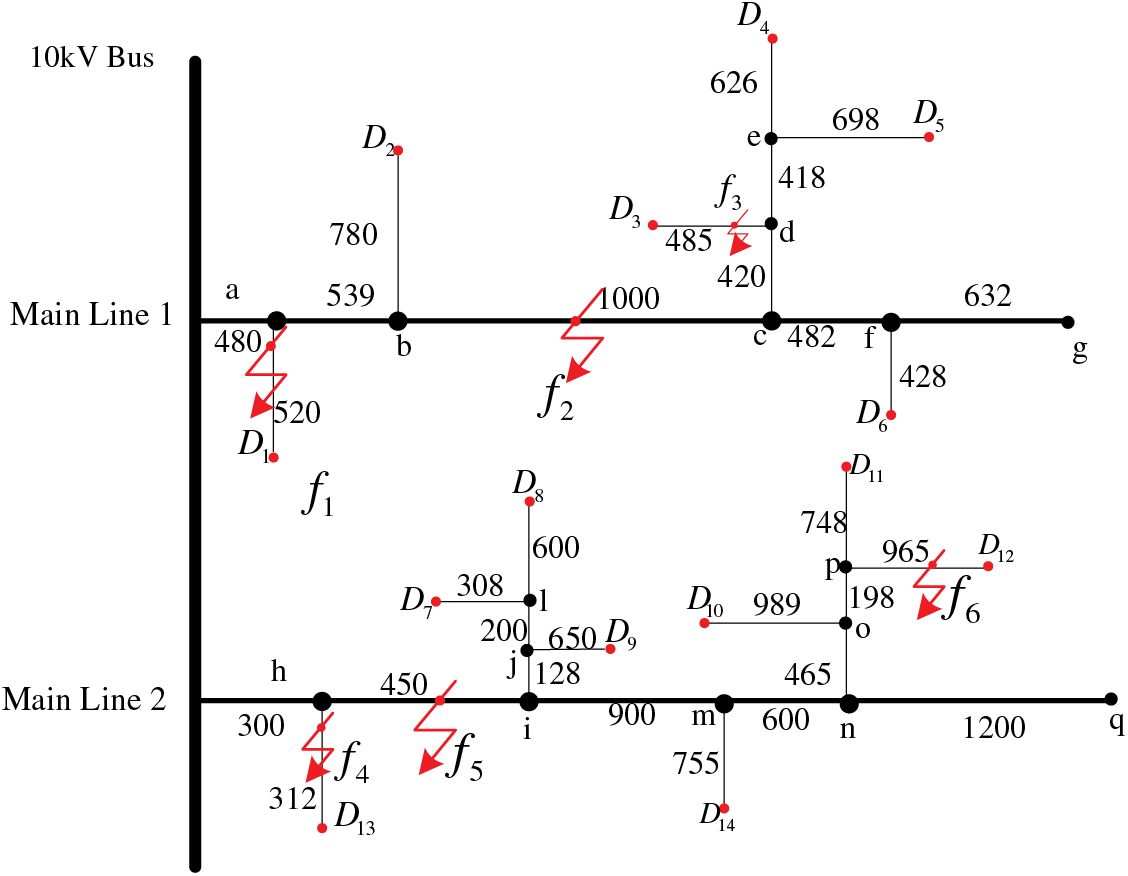
Figure 1: Network structure topology of 10 kV distribution network

In the multi-branch distribution network, there are three main types of line faults. These include mainline faults f2 and f5 (as shown in Fig. 1), single branch faults f1 and f4 (as shown in Fig. 1), and multi-branch faults f3 and f6 (also shown in Fig. 1). The distribution network consists of various branch lines, including T-branch lines and three-branch lines or more [20]. Consequently, accurately locating faults becomes challenging. Based on the difficulty of locating fault branches of multi-branch lines, this paper proposes to decompose multi-branch lines first, to decompose complex lines into only T-branch and three-branch lines, and then build a time difference matrix method on the decomposed lines to locate the fault segments.

In summary, multi-branch lines in Fig. 1 are decomposed, as shown in Figs. 2 and 3 below.

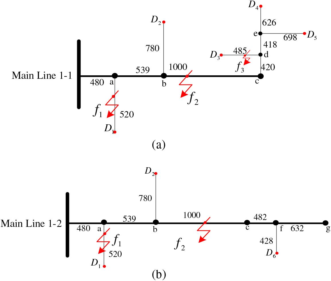
Figure 2: The mainline 1 is broken down into single branch lines

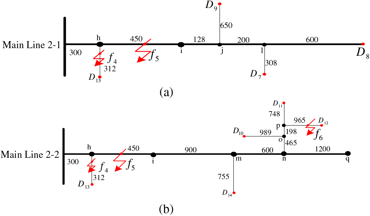
Figure 3: The mainline 2 is broken down into single branch lines

After decomposing the multi-branch line into a simple line (T-branch or three-branch line), the problem of locating faults in complex multi-branch lines is transformed into locating faults in double-ended networks [21]. The main challenge lies in determining the fault segment and accurately pinpointing the fault location using the principle of double-ended traveling wave location.

2.2 Base Time Difference Matrix of Endpoints Is Established

As shown in Fig. 2, when the simulated fault point is set at the head of the mainline 1-1, we use a traveling wave acquisition device to determine the arrival time of the original traveling wave head. The predetermined time for the original traveling wave head to reach the head of the mainline 1-1 as t1−1−1′. The time for the original traveling wave head to reach the end of the mainline 1-1 fault as t1−1−n′, the time for the original fault-traveling wave head to reach the end of other branches as t1−1−2″, t1−1−3″, t1−1−4″,…, t1−1−n−1″, then calculate the difference between the original arrival time of the fault-traveling wave at the end and the arrival time of the other endpoints. When the simulated fault point is set at the end of the mainline 1-1, set the time of the traveling wave head to arrive at the head of the mainline 1-1 as t1−1−1″, the time for the original traveling wave head to reach the end of the fault of mainline 1-1 as t1−1−n″, the time for the original fault-traveling wave head to reach the end of other branches as t1−1−2″, t1−1−3″, t1−1−4″,…, t1−1−n−1″. Calculating the difference between the original arrival time of the fault-traveling wave at the head and the arrival time at other endpoints. Similarly, set the simulated fault point at both ends of mainline 1-2 and use the same method to determine the arrival time of the original traveling wave on mainline 1-2. The difference in arrival time between the original traveling wave head at the beginning and end of mainline 1-2, as well as other endpoints, is calculated. The resulting baseline time difference matrix for the endpoints is shown below:

s1=[t1−1−n′−t1−1−1′t1−1−n′−t1−1−2′…t1−1−n′−t1−1−n−1′00t1−1−1″−t1−1−2″…t1−1−1″−t1−1−n−1″t1−1−1″−t1−1−n″t1−2−n′−t1−2−1′t1−2−n′−t1−2−2′…t1−2−n′−t1−2−n−1′00t1−2−1″−t1−2−2″…t1−2−1″−t1−2−n−1″t1−2−1″−t1−2−n″](1)

Similarly, we can establish the baseline time difference matrix S2 for the endpoints of mainlines 2-1 and 2-2 using the following method:

s2=[t2−1−n′−t2−1−1′t2−1−n′−t2−1−2′…t2−1−n′−t2−1−n−1′00t2−1−1″−t2−1−2″…t2−1−1″−t2−1−n−1″t2−1−1″−t2−1−n″t2−2−n′−t2−2−1′t2−2−n′−t2−2−2′…t2−2−n′−t2−2−n−1′00t2−2−1″−t2−2−2″…t2−2−1″−t2−2−n−1″t2−2−1″−t2−2−n″](2)

2.3 The Establish of the Fault-Traveling Wave Time Difference Matrix

When a genuine fault occurs, we can construct the fault-traveling wave time difference matrix G1. This is done by using traveling wave acquisition devices to record the time when the original fault-traveling wave reaches each endpoint. Suppose the time for the original fault-traveling wave head to reach the head of the mainline 1-1 is tf1−1−1, the time for the original fault-traveling wave to reach the end of the mainline 1-1 is tfn−1−1, the time it takes for the fault-traveling wave to arrive at the end of other branches are tf2−1−1, tf3−1−1, tf4−1−1,…, tfn−1−1−1. Calculating the time difference between the arrival of the original fault-traveling wave at the head of the mainline 1-1 and its arrival at other endpoints. Similarly, set simulated fault points at both the head and end of mainline 1-2, and use the same method to determine the arrival time of the original fault-traveling wave for mainline 1-2. The reach time difference of the original traveling wave head between the head and end of the mainline 1-2 and other endpoints are calculated, respectively, and the fault-traveling wave time difference matrix G1 is acquired as follows:

G1=[tfn−1−1−tf1−1−1tfn−1−1−tf2−1−1…tfn−1−1−tfn−1−1−100tf1−1−1−tf2−1−1…tfn−1−1−tfn−1−1−1tf1−1−1−tfn−1−1tfn−1−2−tf1−1−2tfn−1−2−tf2−1−2…tfn−1−2−tfn−1−1−200tf1−1−2−tf2−1−2…tfn−1−2−tfn−1−1−2tf1−1−2−tfn−1−2](3)

Similarly, the failure time difference matrix G2 of the mainline 2-1 and 2-2 can be established as follows:

G2=[tfn−2−1−tf1−2−1tfn−2−1−tf2−2−1…tfn−2−1−tfn−1−2−100tf1−2−1−tf2−2−1…tfn−2−1−tfn−1−2−1tf1−2−1−tfn−2−1tfn−2−2−tf1−2−2tfn−2−2−tf2−2−2…tfn−2−2−tfn−1−2−200tf1−2−2−tf2−2−2…tfn−2−2−tfn−1−2−2tf1−2−2−tfn−1−2](4)

2.4 Time Difference Matrix Positioning Principle

The transmission characteristics of fault-traveling waves are different between the fault and non-fault lines: As shown in Fig. 1, when the f1 point fails, the original fault-traveling wave will spread throughout the entire distribution network at the speed of light [22]. The location and transmission path of the fault point varies, causing regular changes in the time difference of the traveling wave within the system [23]. The original traveling wave on the non-fault lines originates from the fault line [24]. The transmission path on the non-fault line is not influenced by the location of the fault point [25]. As a result, the time difference of the original traveling wave on the non-fault line remains unchanged compared to before the fault occurred. Therefore, when disregarding detection errors, the elements of row vectors (S1,S2,S3,…,Sn) and (G1,G2,G3,…,Gn) in the reference time difference matrix S are identical to those in the fault time difference matrix G for the non-fault line endpoint. Because the location of the simulated fault point is different from that of the real fault point, the elements of the corresponding row vector of the two matrices are different. When a real fault occurs in the bus bar, the bus bar becomes the traveling wave source for both fault and non-fault lines. Therefore, all elements in matrix S and matrix G for all lines are equal. According to the arrival time of the original traveling wave head, the change rule of elements in matrix S and G can be expressed as Eq. (5).

{Si≠GiLine i is a faulty lineSj=GjLine j is a non-fault line(5)

In Eq. (5), i,j=1,2,3,…,n.

If the elements in the matrix S and G of all lines are the same, it can be judged the bus is faulty.

In a multi-branch distribution network, the mainlines containing multiple branches are decomposed into multiple lines containing only simple branches. A simulated fault point is set at the head and tail of each mainline after decomposition, and the endpoint reference time difference matrix Si and Gi, and the fault time difference matrix of each mainline, are established. The least square method is introduced to find the first-order matching relationship about the corresponding row Sik and Gik of the Si and Gi matrix: Gik=a+bSik,k=1,2,3,…,n. The unequal elements of the corresponding row vectors form the sets A and B. Thus, we can form the complement of the union sets A and B, and the nodes in the complement are used for the multi-branch fault branch location.

3  Research on Fault Location Algorithm of Multi-Branch in the Distribution Network

3.1 Fault Branch Location Algorithm of Multi-Branch Lines

3.1.1 Mainline Fault

According to the above principles, when the fault f2 occurs in Fig. 2a, from the node b to the left of the point of failure, the elements of the corresponding row vector S1k and G1k elements are the same, then take the equal elements of corresponding row vectors S1k and G1k to form the set A={a,b}, from the node c to the right of the point of failure, the elements of the corresponding row vector S1k and G1k are the same, then take the equal elements of corresponding row vectors S1k and G1k in the two matrices to form the set B={c,d,e}, acquire the complement of the union sets A and B according to Eq. (6) below:

H1=∁U(AUB)(6)

In Eq. (6): ∁U as a symbol of the complementary set.

By using Eq. (6), we can determine that if the complement of the union sets A and B is empty, then the fault point lies on the mainline. The relevance degree of elements in sets A and B is measured by distance—the closer the distance, the lower the relevance degree. The fault section is identified by selecting two nodes with the least correlation degree from sets A and B.

3.1.2 Single Branch Fault

A single branch line refers to a branch line that does not have any other branches connected to it. For example, when the fault f1 occurs in Fig. 2a, the original fault-traveling wave spreads from node A to both ends of the mainline. Based on this principle, the corresponding elements of row vectors S1k and G1k for all nodes from A to the left and right are equal. Therefore, there are A={∅} and B={b,c,d,e}, and the complement H={a} of the union of A and B is taken according to Eq. (6). In summary, the fault section is a-D1.

3.1.3 Multiple Branch Fault

When the fault f6 occurs in Fig. 3b, because it occurs on the multi-branch line, there are A={h,i,m} and B={q} after the analysis of the above principle, and thus there is the complement H={n,o,p} of the union of A and B. We can determine that the original fault-traveling wave diffuses from node n to both ends of the mainline. In this case, n-D11 is taken as the new mainline, and at the head n and the tail of D11, re-establish the endpoint reference time difference matrix S and the fault time difference matrix G, The set A={n,o}, B={ϕ}, H={p} can be acquired, so the fault segment is p-D12. In summary, if there are multiple nodes in set H, we need to reset the matrices S and G. We should then repeatedly assess the fault node until only one remains in set H. This process helps us determine the fault segment.

3.2 Fault Point Determination

The original traveling wave head is transmitted along the shortest path, carrying information about the time it takes for the traveling wave from the fault point to reach the detection device [26]. This locating method solely relies on time to identify faults. The difficulty in locating the fault lies in accurately judging the branch of the fault. To obtain the correct algorithm for fault location, this paper decomposes the mainline with multiple branches into several mainlines with only single branches, as shown in Figs. 2 and 3 above.

When a fault point as shown in Fig. 2a occurs, take the f3 fault point as an example, select the two endpoints D4 and D5 that are closest to the endpoint D3. The time of the original fault-traveling wave arrives at the endpoints D3, D4 and D5 is tD3, tD4 and tD5, respectively. The theory of double-ended traveling wave positioning is used for precise fault point location, as shown in Eqs. (7)–(9):

x′=(tD4−tD3)V−Le−f−D4+Le−D32(7)

x″=(tD5−tD3)V−Le−f−D5+Le−D32(8)

x=x′+x″2(9)

In Eq. (7): x′ is by using the endpoint D3 and the D4 fault point is from node e; V is the traveling wave velocity; Le−f−D4 indicates the shortest distance from node e to f to endpoint D4; Le−D3 is the distance between node e and endpoint D3. In Eq. (8): x″ is by using endpoint D3 and D5 fault point is from the partial node e; Le−f−D5 is the shortest distance from node e to f to the endpoint D5. In Eq. (9): x is the average distance from the fault point to the node e.

The velocity of the traveling wave is not solely determined by the speed of light, as it is influenced by line parameters. In this paper, we combine two data points from the fault time difference matrix G that have the minimum time difference for each line. We use these data points to calculate the wave velocity based on the principle of original fault-traveling wave diffuseness along the shortest path. Finally, we average out the sum of wave velocities acquired from each line, as shown in Eqs. (10) and (11):

Vi=(L1min−L2min)/(Δt1−Δt2),i=1,2,3,…,n(10)

V=∑i=1nVin(11)

In the above formula, Vi is the wave velocity calculated by each row, Δt1 and Δt2 are the two data with the smallest time difference corresponding to each row of the matrix G, the L1min and L2min are the shortest transmission distance of fault-traveling wave corresponding to Δt1′ and Δt2, respectively, and V is the traveling wave velocity.

3.3 Segment-Location Algorithm Based on Least Square Data Fitting

Based on the principles mentioned above, the matrix S and G of a non-fault line should be identical under ideal circumstances. However, in practical situations, various measurement errors occur. For instance, factors like interference, lightning strikes, and high-frequency signals can affect the traveling wave acquisition device. As a result, incorrect original traveling wave heads are identified during fault identification. The arrival time of the calibration original traveling wave head shows varying degrees of error. To mitigate this, we introduce the least square method for a one-time fitting to reduce the impact of errors.

The least square method is a mathematical technique used for fitting data. Specifically, the linear least square method determines if the data follows a linear pattern and finds the best function that fits the data by minimizing the sum of squared errors [26]. This method allows for easy estimation of unknown data points and minimizes discrepancies between acquired and actual data.

The linear least square method is used to find a linear relationship between x and its corresponding y. The equation for this method is:

y=a+bx(12)

The undetermined constants a and b in the equation are transformed into linear regression coefficients, which represent the intercept and slope of the line. The goal of the fitting is to determine these regression coefficients based on measured data, to minimize deviation and to make data points as close as possible to the straight line. Deviations can be positive or negative, and their calculation follows this formula:

s=∑i=1nvi2=∑i=1n(yi−a−bxi)2(13)

When S is the smallest in the above equation, the corresponding a represents the fitted curve coefficient. Both a and b must satisfy the following conditions:

{a=y−−bx−→0b=∑i=1n(xi−x−)(yi−y−)∑i=1n(xi−x−)2→1(14)

In Eq. (14): b is a slope deviation; a is a displacement deviation degree; x− is the arithmetic mean value of the data in variable X, and y− is the arithmetic mean value of the data in variable Y.

The first-order fitting relation obtained through the least square method must satisfy the matching relation between the corresponding row vectors and the subfunction (Gik=a+bSik) of the line. If Eq. (14) is satisfied after a one-time fitting, it indicates that the elements in row vectors Sik and Gik of the matrix Si and Gi have undergone a successful linear fitting process. In this case, the node can be considered non-faulty. If it is not functioning properly, it can be considered a faulty node. To minimize the error, we can use least squares to fit each row in the matrix Si and Gi, allow for a more precise determination of the faulty node.

Fig. 4 illustrates the process of locating a fault on a multi-branch route when it occurs.

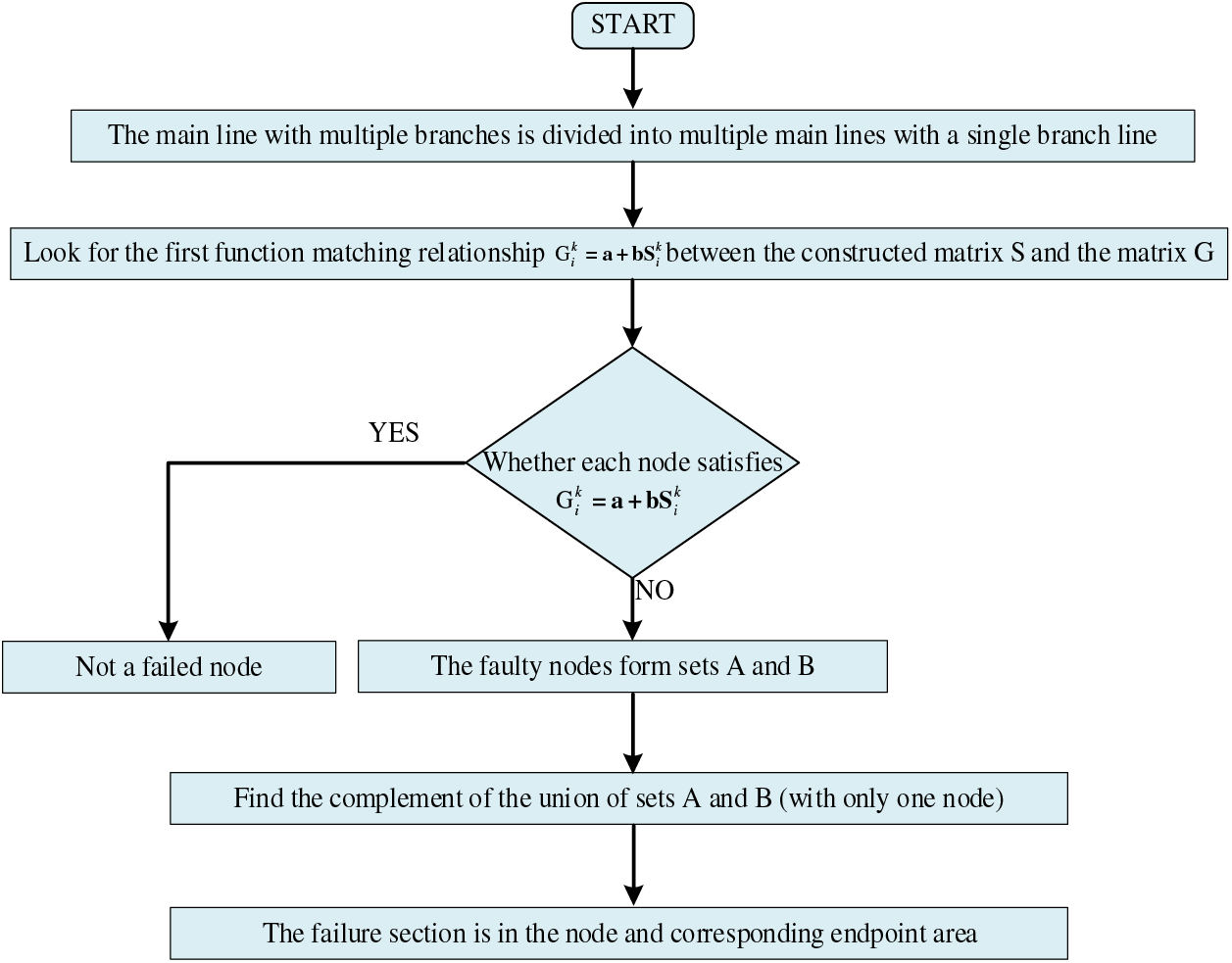
Figure 4: The process of locating a fault on a multi-branch route

4  Simulation Verification

4.1 Verification of Fault-Traveling Wave Location Algorithm

The multi-branch distribution network, depicted in Fig. 1, was constructed using PSCAD. The fault was programmed to occur at f6.

The S2 matrix of mainline 2 is (the unit of matrix elements is μs) as follows:

S2=[himnopq9.845.615.70−0.98−1.49−0.71000.0811.851.661.192.356.2815.5613.5110.278.934.81−0.7800−0.04−0.26−1.615.696.589.24](15)

After a fault occurs, the traveling wave detection device constructs the original time of the fault-traveling wave head using the fault time difference matrix G from mainline 2, as shown in Eq. (16).

G2=[himnopq−2.61−1.90−0.90−2.191.706.3200−1.91−4.52−6.68−10.83−15.92−14.091.253.287.1815.1220.70−18.11004.29−12.298.694.869.477.84](16)

The row vectors S2k and G2k of the matrix S2 and G2 were fitted using least squares. The fitting results can be seen in Figs. 5 and 6 below.

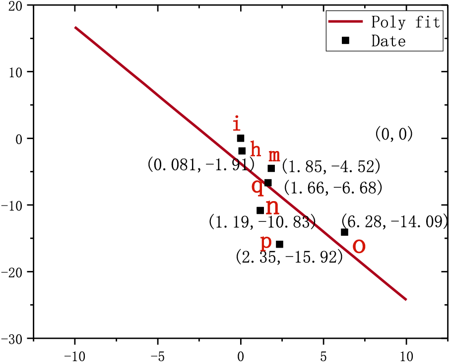
Figure 5: The linear fitting diagram of S21 and G21

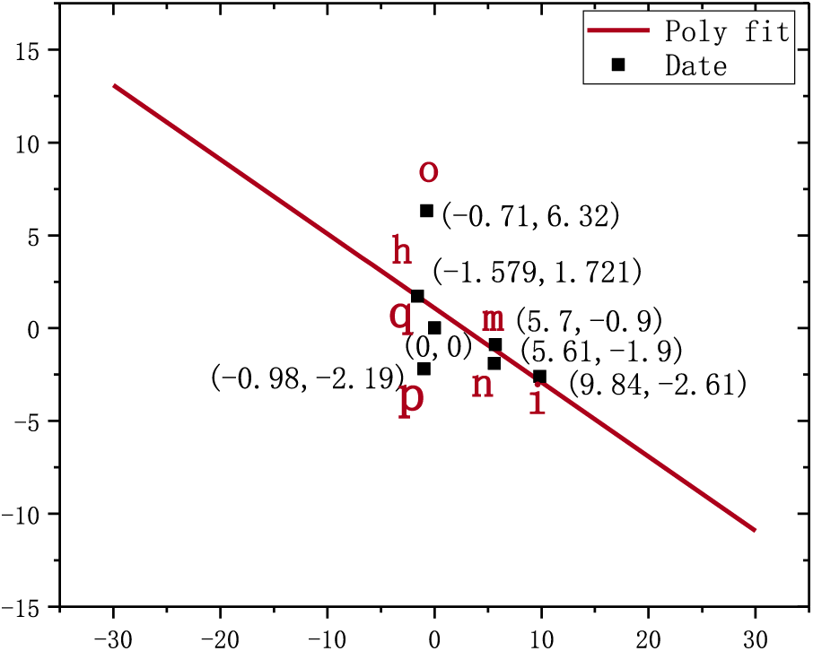
Figure 6: The linear fitting diagram of S22 and G22

As shown in Figs. 5 and 6, when the elements of the corresponding row vectors in the matrix S2 and G2 satisfy the first-order fitting relation, The A={q} and B={h,i,m} can be acquired. The complement set of the union sets A and B can be used to acquire H={n,o,p}. so the fault section is n-D11. Since the fault occurs on a multi-branch line, we set a new simulated fault point at the new head and designated D11 as the new end. Two matrices are established as follows: a new endpoint reference time difference matrix (matrix S′) and a fault-traveling wave time difference matrix (matrix G′).

S′=[nop−1.560.5806.289.840](17)

G′=[nop08.320.360−14.09−18.10](18)

As shown in Figs. 7 and 8, there are the A={n} and B={o}, then we can acquire the complement H={p} of the union of A and B, thus the fault section is p-D12.

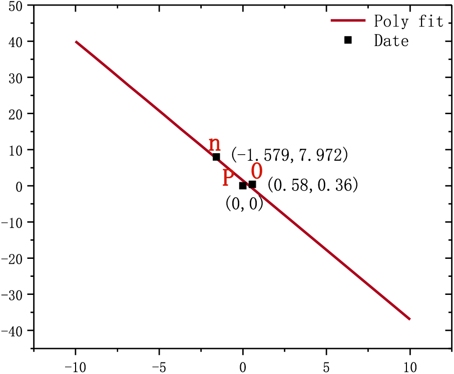
Figure 7: The linear fitting diagram of S′1 and G′1

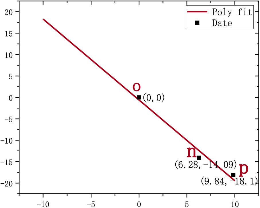
Figure 8: The linear fitting diagram of S′2 and G′2

4.1.1 The Influence of Different Transition Resistors

To analyze the impact of transition resistance on this multi-branch fault location algorithm, we conducted experiments with different ground fault types and fault points. Specifically, we tested fault resistances of 50, 500, and 1000 Ω, respectively. Additionally, we set the original phase of the faults to 90° and introduced white noise with a signal-to-noise ratio of 40 dB as a jamming signal. The results of fault location are shown in Table 1.

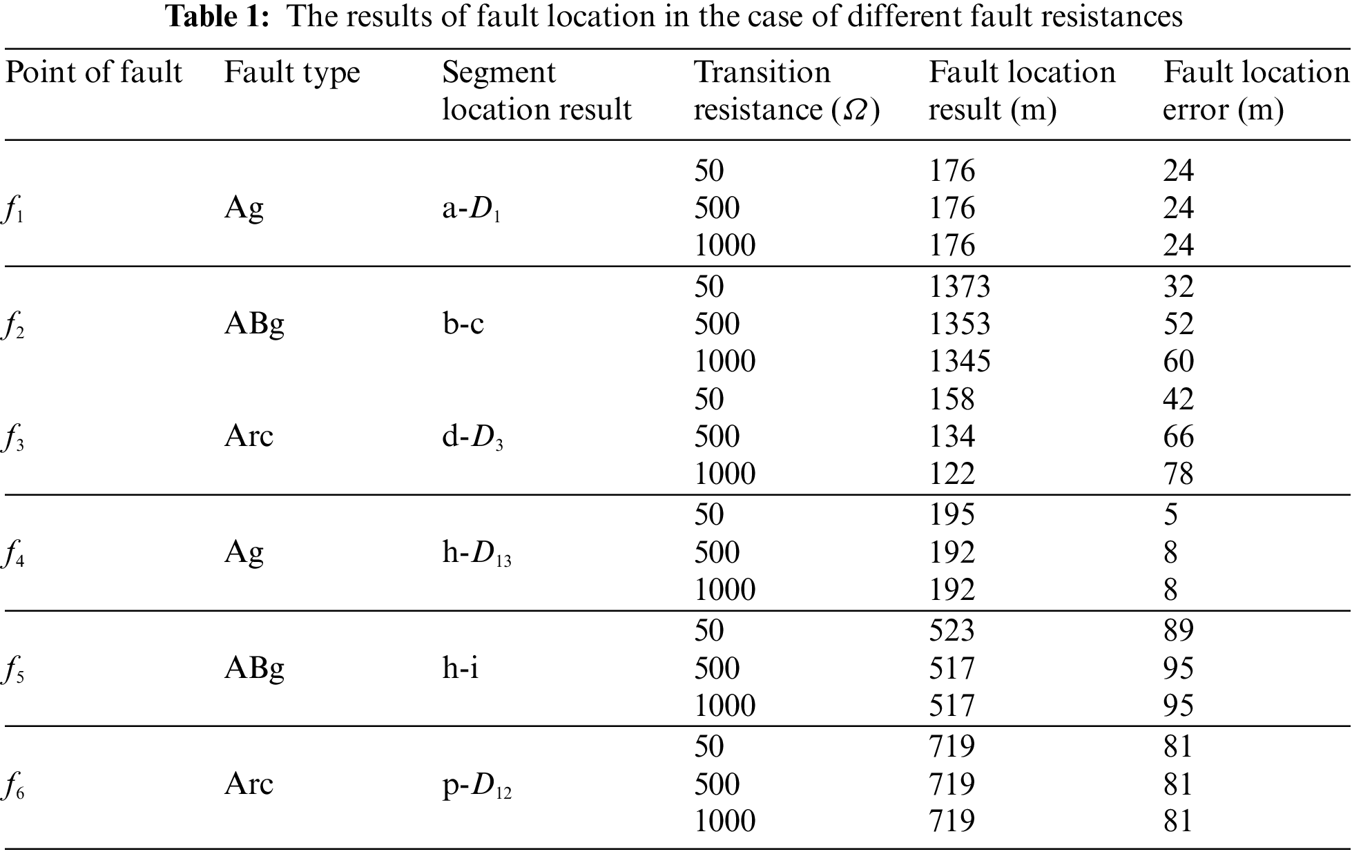
It can be acquired from the results in Table 1 that: The multi-branch fault location method can accurately identify the fault section and locate the fault point even in the presence of white noise interference. However, as the fault resistance increases, there may be a slight increase in the error range. Nonetheless, overall, the influence of fault resistance on this method’s accuracy is minimal.

4.1.2 The Influence of Different Fault Original Phase Angle

To analyze the impact of the original fault phase angle on this multi-branch fault location algorithm, we conducted simulations with different ground fault types and fault points. Specifically, we tested three scenarios: 30°, 60°, and 90° fault phase angles. In each scenario, we set the fault resistance to 50 Ω and introduced a white noise interference signal with a signal-to-noise ratio of 40 dB for accurate simulation. The results of fault location are shown in Table 2.

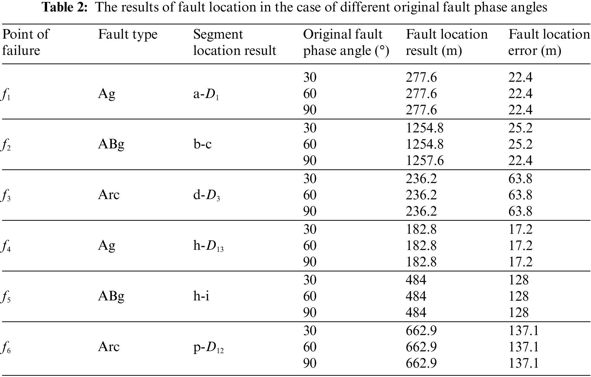
It can be acquired from the results in Table 2 that: The multi-branch fault location method can accurately determine the fault section and locate the fault point even in the presence of white noise interference. Additionally, increasing the fault original phase angle reduces the fault error, while different fault original phase angles have minimal impact on the accuracy of the fault location results.

4.1.3 The Effect of Different Noises

To analyze the influence of white noise on this fault location algorithm, we added white noise signals to the sampled signal. The signal-to-noise ratios used were 40, 50, and 60 dB. For simulation purposes, we set the fault resistance at 50 Ω and the fault original phase angle at 90°. The results of fault location are shown in Table 3.

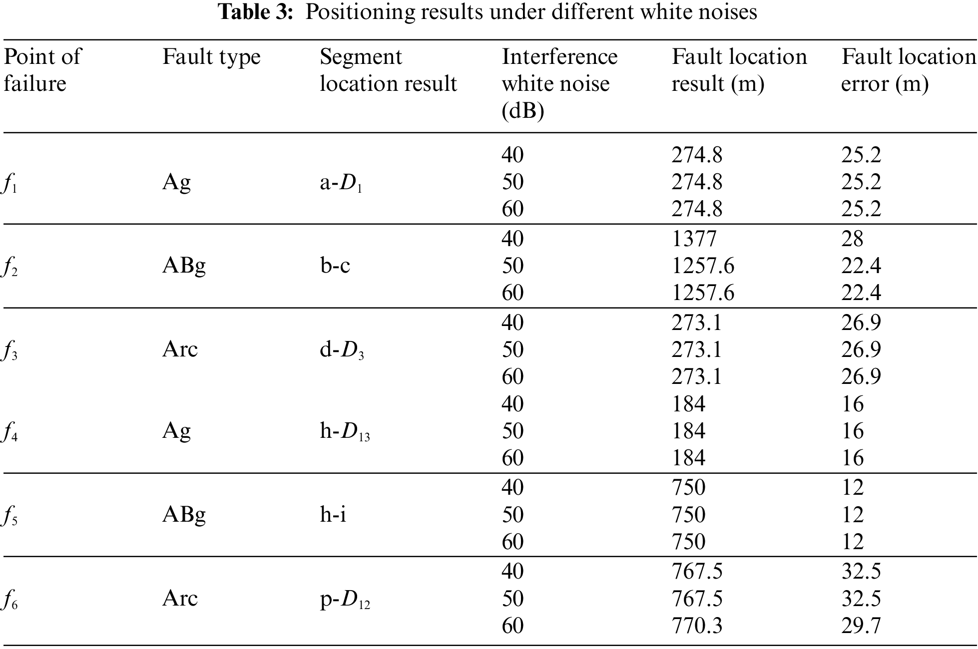
It can be acquired from the results in Table 3 that: This fault location method can accurately identify the faulty branch in the presence of various white noise interference signals, enabling precise fault point localization. As the signal-to-noise ratio increases, the fault location error gradually decreases, and white noise has minimal impact on the accuracy of fault location results.

4.2 Comparison of Different Methods

We analyzed the positioning effects of various methods. Based on the fault locations and types shown in Fig. 1, we used the method proposed in reference [27] to locate the faults. The fault location results obtained from both reference [27] and our method are displayed in Fig. 9, with the x-axis representing the fault points and the y-axis indicating the corresponding fault location results.

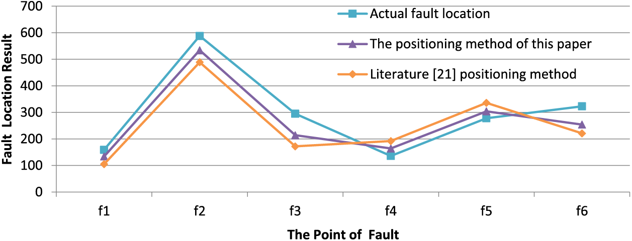
Figure 9: Positioning errors of different methods

Fig. 9 shows that both the method described in the literature and the method proposed in this paper can accurately locate faults in multi-branch distribution networks. However, the method from reference [21] has a maximum fault location error of 182 m and an average error of 86.58 m. In contrast, our proposed method has a maximum error of 150 m and an average error of 57.08 m. Therefore, our method significantly improves fault location accuracy for multi-branch distribution networks compared to existing methods mentioned in the literature.

5  Conclusion

The fault location problem in the multi-branch distribution network can be addressed by decomposing the multi-branch mainline into multiple mainlines with single branches. This transforms the multi-branch fault location problem into a double-ended fault location problem. To determine the fault segment, we establish an endpoint time difference matrix and a fault time difference matrix based on the propagation features of the fault-traveling wave in both fault and non-fault lines. By comparing the change rules of corresponding elements in these matrices, we can identify the faulty section. Additionally, to improve practicality, we introduce a least square fitting model to reduce errors caused by marking the original traveling wave head, lightning strikes, or high-frequency noise. This method enhances engineering applicability and is suitable for addressing faults in multi-division power grid systems. In summary, this paper proposes a logical and orderly location method that observes matrix features before and after a fault to handle faults in multi-branch lines. However, it relies on improvements in traveling wave acquisition equipment performance and clock synchronization device accuracy.

Acknowledgement: The authors acknowledge the support of State Grid Hunan Electric Power Research Institute.

Funding Statement: This work was funded by the project of State Grid Hunan Electric Power Research Institute (No. SGHNDK00PWJS2210033).

Author Contributions: The authors confirm their contribution to the paper as follows: The study conception and design: Hua Leng, Silin He; data collection: Silin He, Jian Qiu; analysis and interpretation of results: Feng Liu, Xinfei Huang; draft manuscript preparation: Xinfei Huang, Jiran Zhu. All authors reviewed the results and approved the final version of the manuscript.

Availability of Data and Materials: Data supporting this study are included within the article.

Conflicts of Interest: The authors declare that they have no conflicts of interest to report regarding the present study.

References

1. Xu, F., Dong, X. Z., Wang, B., Shi, S. X. (2015). Single-ended assembled fault location method and application considering secondary circuit transfer characteristics. Proceedings of the CSEE, 35(20), 5210–5219. [Google Scholar]

2. Deng, F., Zeng, X. J., Ma, S. C. (2017). Research on wide area traveling wave fault location method based on distributed traveling wave detection. Power System Technology, 41(4), 1300–1306. [Google Scholar]

3. Mahamedi, B., Sanaya-Pasand, M., Azizi, S. (2015). Unsynchronised fault location technique for three-terminal lines. IET Generation Transmission & Distribution, 15(9), 2099–2107. [Google Scholar]

4. Nanayakkara, O., Rajapakse, A., Wachal, R. (2012). Location of DC line faults in conventional HVDC systems with segments of cables and overhead lines using terminal measurements. IEEE Transactions on Power Delivery, 27(1), 279–288. [Google Scholar]

5. Korkali, M., Lev-Ari, H., Abur, A. (2011). Traveling-wave-based fault location technique for transmission grids via wide-area synchronized voltage measurements. IEEE Transactions on Power Systems, 27(2), 1003–1011. [Google Scholar]

6. Deng, F., Li, X. R., Zeng, X. J. (2018). Research on single-end traveling wave based protection and fault location method based on waveform uniqueness and feature matching in the time and frequency domain. Proceedings of the CSEE, 38(5), 1475–1487. [Google Scholar]

7. He, L. J., Shi, C. K., Yan, Z. (2017). A fault section location method for small current neutral grounding system based on energy relative entropy of generalized S-transform. Transactions of China Electrotechnical Society, 32(8), 274–280. [Google Scholar]

8. Liang, R., Yang, X. J., Xue, X. (2015). Study of accurate single-phase grounding fault location based on the distributed parameter theory using data of zero sequence components. Transactions of China Electrotechnical Society, 30(12), 472–479. [Google Scholar]

9. Zhang, K., Zhu, Y. L., Zheng, Y. Y., Liu, S. (2019). Multi-branch hybrid line fault location method based on redundancy parameter estimation. Grid Technology, 43(3), 1034–1040. [Google Scholar]

10. Li, C. B., Tan, B., Gao, P. (2013). A fault location method for T-connection lines based on D-type traveling wave theory. Power System Protection and Control, 41(18), 78–82. [Google Scholar]

11. Chen, X., Zhu, Y. L., Zhao, X. S. (2015). Traveling wave fault location for T-shaped transmission line considering a change of line length. Power System Technology, 39(5), 1438–1443. [Google Scholar]

12. Fan, X. Q., Zhu, Y. L. (2013). A novel fault location scheme for multi-terminal transmission lines based on the principle of double-ended traveling waves. Power System Technology, 37(1), 261–269. [Google Scholar]

13. Pang, Q. L., Ye, L., Ma, Z. X., Zheng, Y. (2022). Traveling wave fault location for multi-branch small current grounding system based on VMD-TEO. Science Technology and Engineering, 22(27), 11943–11950. [Google Scholar]

14. Wang, B., Jiang, Q. Y., Gu, W. (2013). A novel fault location method is suitable for transmission lines with multiple branches. Power System Technology, 37(4), 1152–1158. [Google Scholar]

15. Gend, J. Z., Wang, B., Dong, X. Z. (2015). A novel one-terminal single-line-to-ground fault location algorithm in transmission line using post-single-phase-trip data. Transactions of China Electrotechnical Society, 30(16), 184–193. [Google Scholar]

16. Wang, Q., Jin, T., Mohamed, M. A. (2021). A fast and robust fault section location method for power distribution systems considering multisource information. IEEE Systems, 16(2), 1954–1964. https://doi.org/10.1109/JSYST.2021.3057663 [Google Scholar] [CrossRef]

17. Jin, T., Zhuo, F., Mohamed, M. A. (2020). A novel approach based on CEEMDAN to select the faulty feeder in neutral resonant grounded distribution systems. IEEE Transactions on Instrumentation and Measurement, 69(7), 4712–4721. [Google Scholar]

18. Wang, Q., Jin, T., Mohamed, M. A. (2021). A novel linear optimization method for section location of single-phase ground faults in neutral non effectively grounded systems. IEEE Transactions on Instrumentation and Measurement, 70, 1–10. [Google Scholar]

19. Wang, Q., Jin, T., Mohamed, M. A. (2019). An innovative minimum hitting set algorithm for model-based fault diagnosis in power distribution network. IEEE Access, 7, 30683–30692. [Google Scholar]

20. Fu, H., Wang, J. Y. (2021). Weak fault-traveling wave detection method based on SR-VMD. Power System Protection and Control, 49(1), 156–162. [Google Scholar]

21. Elkalashy, N. I., Otaibi, S. A., Elsayed, S. K., Ahmed, Y., Hendawi, E. (2021). Earth fault management for smart grids interconnecting sustainable wind generation. Intelligent Automation & Soft Computing, 28(2), 477–491. https://doi.org/10.32604/iasc.2021.016558 [Google Scholar] [CrossRef]

22. Zeng, H. A., Rezk, H., Al-Dhaifallah, M. (2021). Accurate fault location modeling for parallel transmission lines considering mutual effect. Computers, Materials & Continua, 67(1), 491–518. https://doi.org/10.32604/cmc.2021.014493 [Google Scholar] [CrossRef]

23. Wang, C. B., Yun, Z. H., Zhang, H. X. (2019). Parameter-free fault location algorithm for a multi-terminal overhead transmission line of a distribution network based on μ MPMU. Power System Technology, 43(9), 3202–3209. [Google Scholar]

24. Xi, Y. H., Zhang, X. D., Li, Z. W. (2018). Double-ended traveling-wave fault location based on residual analysis using an adaptive EKF. IET Signal Processing, 12(8), 1000–1008. [Google Scholar]

25. Lopesf, V., Dantas, K. M., Silva, K. M. (2018). Accurate two-terminal transmission line fault location using traveling waves. IEEE Transactions on Power Delivery, 33(2), 873–880. [Google Scholar]

26. Evrebosogluc, Y., Abur, A. (2005). Based on the traveling wave for the fault location. IEEE Transactions on Power Delivery, 20(2), 1115–1121. [Google Scholar]

27. Xie, J., Wang, Y., Jin, G., Wu, M. (2022). T-shaped transmission line fault location based on phase-angle jump checking. Energy Engineering, 119(5), 1797–1809. [Google Scholar]