Wind Turbine Spindle Operating State Recognition and Early Warning Driven by SCADA Data

Nomenclature

1  Introduction

In recent years, the rapid expansion of wind power has assumed an increasingly prominent position in the energy structure industry [1]. As a typical mechatronic product, the reliability of wind turbine is particularly essential during the operation due to its function and structure increasing in complexity with the continuously increasing unit capacity [2,3]. Direct drive wind turbines greatly reduce the operation and maintenance costs of wind turbines by omitting the gearbox, meanwhile, the reliability of the spindle draws numerous scholars’ attention, As a critical component inside wind turbine, the spindle not only carries various loads on the wheel hub, but also transmits torque to the rotor, which has an influential effect on the cumulative reliability of wind turbine. Therefore, the operation state recognition and early warning of the spindle can effectively reduce the operation and maintenance cost and downtime of the wind turbine, which is of vital significance to the stable operation of the wind turbine.

The approaches of wind turbine operational condition monitoring include vibration signal monitoring [4], electrical signal monitoring [5] and SCADA data monitoring [6]. In terms of vibration signal monitoring, reference [7] represented the vibration signal by multi-scale dictionary method to effectively extract the vibration signal for condition monitoring of wind turbine drive train. Reference [8] proposed a fault diagnosis strategy with excellent noise immunity through convolutional neural network combined with random forest. As for electrical signal monitoring, reference [9] developed an electromechanical model of a wind turbine with an integrated drive train fault model based on electrical signals. Reference [10] employed a synchronous resampling algorithm to process the non-stationary current signals for quantitative assessment of the wind turbine health status. While the above researches require the installation of a large number of sensors for signal acquisition, the failure of sensors not only reduces the reliability of the collected data, but also increases the additional operation and maintenance costs. In addition, the electrical signal acquisition of failure data information is usually weak, which generates significant inaccuracies in monitoring results. In recent years, the wind turbine monitoring driven by SCADA data has gradually emerged as a research hotspot in the field of wind turbines [11]. Reference [12] constructed a data-driven deep convolutional neural network modeling framework for condition monitoring and performance prediction of wind turbines. Reference [13] adopted support vector machine to train a fault classifier for early fault detection and classification of bearings. Reference [14] employed LightGBM method to construct wind turbine condition monitoring and fault recognition model by adding condition labels based on SCADA data. Since the above researches require tagging a large amount of historical failure data, which is tedious and time-consuming, and the SCADA system of in-service wind turbines exports few failure data, which is difficult to be promoted and utilized in realistic monitoring of key wind turbine components.

Therefore, this work proposes a research method of wind turbine spindle operation status recognition and early warning driven by SCADA data, which features status identification based entirely on normally operating SCADA data without using any failure data. With the analysis of the SCADA data from a domestic 2.5 MW direct drive wind turbine, the spindle speed is selected as the output parameter for spindle operation status recognition, which focuses on extracting the relevant feature parameters of spindle speed and establishing the prediction model to implement the spindle operation status recognition and failure warning. In this work, Section 2 describes the SCADA data and completes the related data pre-processing work, as well as establishes the spindle speed prediction model. In Section 3, on the basis of interval estimation theory, the operating state index is applied to determine the abnormal state threshold of wind turbine spindle operation, whereby the operating status of wind turbine spindle is identified. In Section 4, this approach is employed in the recognition and early warning analysis of the operating state of a 2.5 MW wind turbine main shaft in a domestic wind farm. Section 5, summarizes the relevant conclusions obtained from this work.

2  SCADA Data Preprocessing

2.1 Data Cleaning

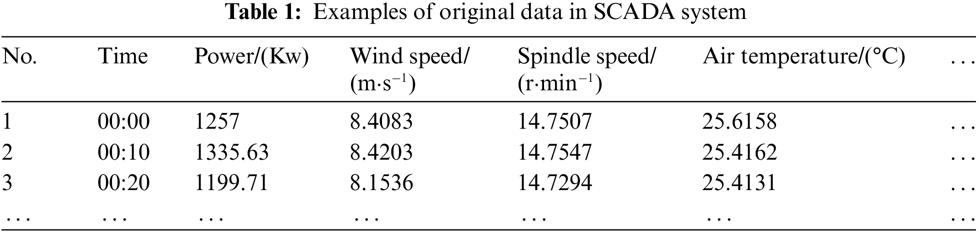
With a domestic wind field F24 wind turbine as the research object, and the total 54607 sets of data from 0:00 on July 01, 2018 to 0:00 on July 01, 2019 selected as the original research data. The SCADA original research data format is shown in Table 1.

In accordance with the wind speed-power characteristic curve and the distribution characteristics of abnormal data, QM-DBSCAN method is utilized to exclude the abnormal data induced by extreme weather, component failure, wind curtailment. QM-DBSCAN is a methodology for identifying and cleaning wind speed-power data. It combines the quartile method (QM) and the density-based spatial clustering of applications with noise (DBSCAN) to carry out the differentiated cleaning of abnormal data according to the category and characteristics of wind speed-power data clusters. The cleaning effect is shown in Fig. 1.

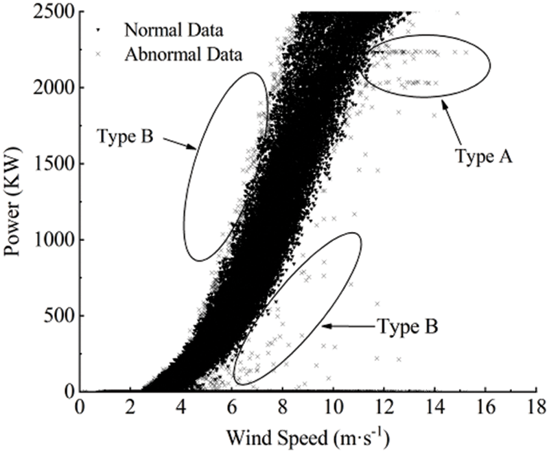
Figure 1: The wind speed-power scatter after data cleaning by the QM-DBSCAN method

As shown in Fig. 1, “●” indicates normal data and “×” represents abnormal data, where the abnormal data of type A is caused by wind abandonment and power limitation, which is manifested as one or more clusters of data parallel to the horizontal axis in the middle of the wind speed-power curve. The anomalous data of type B is generated by extreme weather and unit component failure, showing irregularly scattered points around the wind speed-power curve. By excluding 12,306 sets of abnormal data by this method, the remaining normal data total 42,301 sets.

2.2 Data Normalization

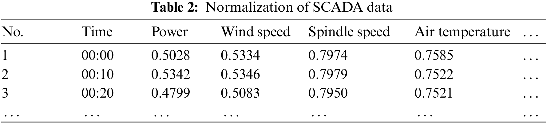
SCADA system captures operating data for 10 min, which mainly comprises monitoring parameters of wind speed, output power and spindle speed, and these parameters have different dimensions and dimensional units. For eliminating the influence of dimensions between parameters, it is necessary to normalize the monitoring data after cleaning. The formula is as follows:

x∗=(xi−x¯)/(1n∑i=1n(xi−x¯)2)(1)

In Eq. (1), xi denotes the i-th data in SCADA data, x¯ is the average of SCADA data, and x∗ indicates the normalized data. The normalized data pattern is listed in Table 2.

2.3 Extraction of Features

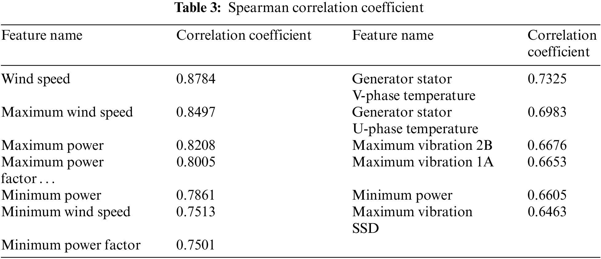
Aiming at the characteristics of large volume, high dimensions and strong redundancy of the data collected by wind turbine SCADA system, the feature extraction of the normalized SCADA data is carried out to eliminate irrelevant parameters, proposing a feature selection approach combining Spearman correlation coefficient and Principal Component Analysis (PCA). The spindle speed indicates the operating state of the spindle, hence the spindle speed is adopted as the output parameter to extract the operating parameters related to the spindle speed, where the Spearman correlation coefficient is as follows:

r=∑i=1n(xi−x¯)(yi−y¯)∑i=1n(xi−x¯)2∑i=1n(yi−y¯)2(2)

In Eq. (2), xi denotes the i-th operating parameters data in SCADA data, and x¯ is the average value of the operating parameters in SCADA data. yi denotes the data of the i-th spindle speed in SCADA data, while x¯ is the spindle average in SCADA data.

Since the operating parameters have a varying influence on the spindle speed, the correlation coefficient between the output parameter spindle speed and the remaining 49 monitoring parameters are calculated by using the method of Spearman correlation coefficient, and the monitoring parameters with correlation coefficients above 0.6 with spindle speed are selected as the initial characteristic parameters, the ranking results are summarized in Table 3.

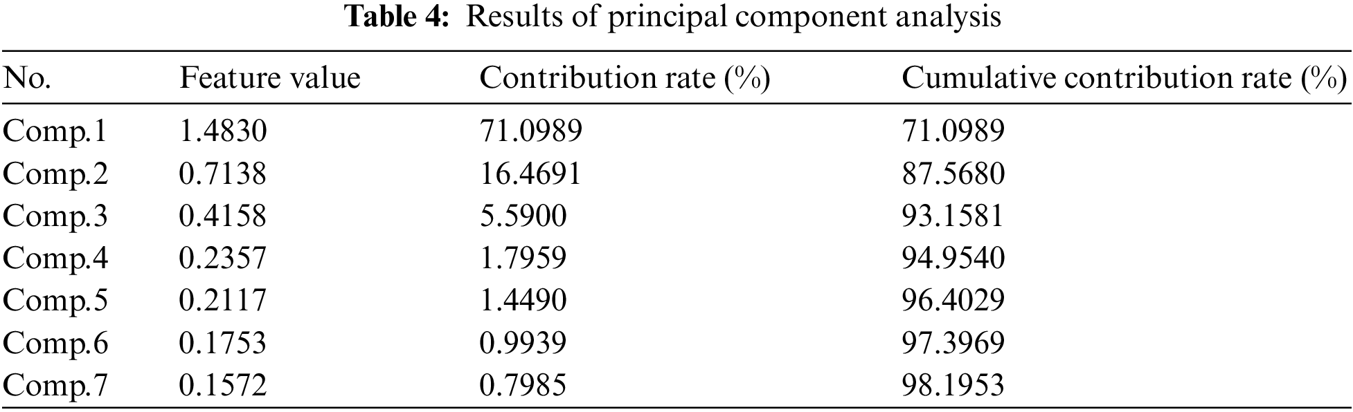
PCA is available within the feature extraction to retrieve further new variables that reflect the original information of all variables and to eliminate redundant information among monitoring data to enhance the prediction accuracy of the model. The feature value, contribution rate and cumulative contribution rate corresponding to each principal component as shown in Table 4, where the feature value refers to the variance of the principal component, and the contribution rate represents the percentage of the original information preserved after the dimension reduction of the primary variable, while the larger of the contribution rate indicates that more original variable information is preserved, whereas the cumulative contribution rate is the sum of the cumulative contribution rate. With the inclusion of 7 principal components, the cumulative contribution rate reached more than 98%, which indicates that the new variables covered over 98% of the information of the original variables, thus transforming the original 13 variables into linearly uncorrelated 7 new variables as the final input of the prediction model.

3  Construction of Prediction Model

3.1 Single Prediction Model

Extreme Learning Machine (ELM) is a novel single-hidden-layer feed-forward neural network learning algorithm [15], which can accomplish the classification and regression of multiple complex tasks by setting fewer grid parameters in training process ELM network consists of input layer, hidden layer and output layer. Its network topology is shown in Fig. 2.

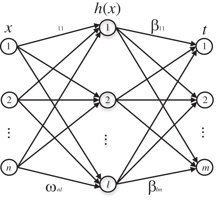
Figure 2: Topology of ELM network

The output function of the hidden layer is defined as follows:

fl(x)=∑i=1lβihi(x)=h(x)β(3)

where x is the input to the neural network, β=[β1,…,βl]T is the output weight between the hidden layer of l nodes and m≥1 output nodes, and h(x)=[h1(x),⋯,hl(x)] is denoted as the feature mapping or activation function, which serves to map the data in the input layer from the original space to the ELM feature space.

hi(x)=G(ai,bi,x)(4)

where ai and bi are the parameters of the feature mapping.

Support Vector Machine (SVM) is a machine learning method with supervision features that solve classification and regression problems [16], In this work, Support Vector Machine Regression (SVR) is employed to construct a loss function between the sample labels and the model prediction values to minimize the loss function and determine the wind turbine spindle speed prediction model.

The SVR learning objective is to find the optimal hyperplane closest to all points at a given interval, y=wTx+b, and its objective function and constraints are

minw,b,ξ,ξ∗12wTw+C∑i=1lξi+C∑i=1lξi∗s.t.   wTϕ(xi)+b−yi≤ε+ξiyi−wTϕ(xi)−b≤ε+ξiξiξi∗≥0,i=1,2,⋯,l}(5)

where w and b are the weight coefficients and bias coefficients for learning the optimal hyperplane, respectively, C is the penalty factor, ξi and ξi∗ are the introduced slack variables, and ε is the given interval.

Elman neural network is a recurrent neural network with local memory units and local feedback connections, which has more capability to deal with dynamically changing data [17], wherein the undertake layer is a specific hidden layer, which receives feedback signals from the hidden layer and then passes forward to the hidden layer through the output of neurons in this layer, completing the local feedback connection and equipping the network with a memory so that the system has the ability to make predictions on time series data, the structure of Elman neural network is shown in Fig. 3.

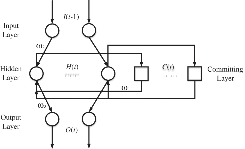
Figure 3: Structure of Elman neural network

At time t the outputs H(t), C(t), and O(t) of the hidden, takeover, and output layers, as follows:

H(t)=f[ω1C(t)+ω2I(t−1)](6)

C(t)=H(t−1)(7)

O(t)=g[ω3H(t)](8)

in which I(t−1) represents the input of the input layer at time t−1 ω1, ω2 and ω3 are weights of the take-up layer, input layer and hidden layer, respectively, whereas f(⋅) and g(⋅) indicate the transfer functions of the neurons in the hidden layer and output layer.

3.2 Combined Prediction Models

Combined prediction models can effectively minimize the effectiveness of the random factors of the singular prediction models, comprehensive the singular prediction models to further improving the accuracy of prediction, Assuming that a prediction problem has n single prediction models, suppose A indicates the predicted value of the combination model consisting of j single prediction models at the i-th point (where, i = 1, 2,…, n; j = 1, 2, …, m), the entropy value method [18] is implemented to construct the combination prediction model, as follows:

(1) Solving the relative error eij between the predicted and monitored values of the j-th prediction model.

eij=|(yi−y^ij)/yi|(9)

(2) Determining the weight of the relative error pij between the predicted and monitored values of the j-th predictive model.

pij=eij/∑j=1meij(10)

(3) Calculating the entropy value of the relative error gj between the predicted and monitored values of the j-th prediction model.

gj=−1ln⁡n∑i=1npijln⁡pij(11)

(4) Solving for the weights of each single prediction model wj.

wj=gj/∑j=1mgj(12)

3.3 Selection of Prediction Model Parameters

A total of 42301 sets of normal SCADA data with seven characteristic parameters obtained after data preprocessing as the input parameters of each prediction model carried out the construction work of wind turbine spindle speed prediction models, by loading elmNNRcpp, E1071, RSNNS through R language platform to construct ELM, SVR, and Elman prediction models. The specific step-by-step flow of each model establishment as shown in Fig. 4.

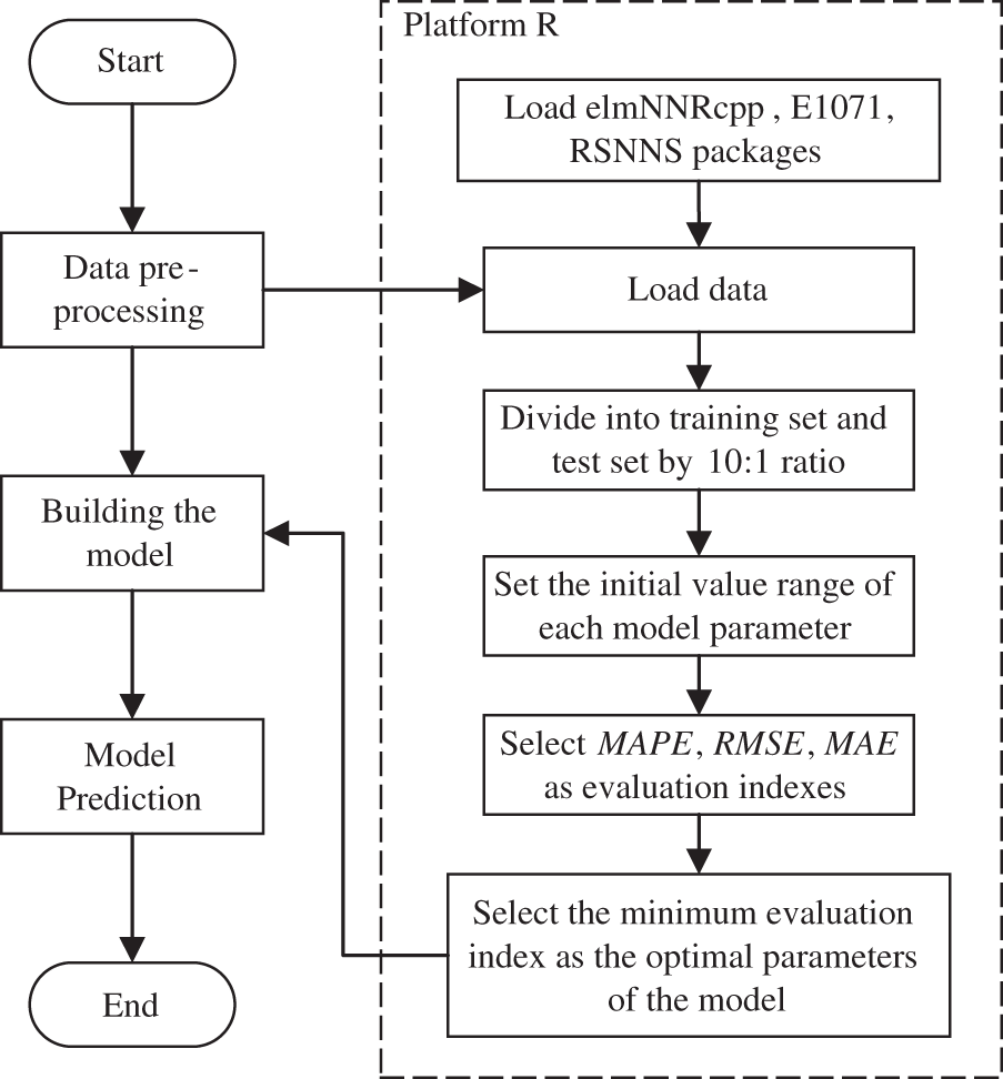
Figure 4: Process of prediction model construction

The optimal parameters of each model trained by the training set data are shown in Table 5.

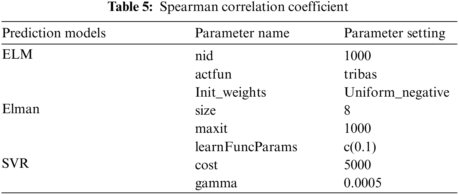
After determining the optimal parameters of each model, the ELM, SVR, and Elman prediction model weights in the combined model are calculated by Eqs. (9)–(12) with 0.4322, 0.1782, and 0.3895, respectively.

3.4 The Evaluation Index of the Prediction Model

With the mean absolute percentage error (MAPE), root mean square error (RMSE), mean absolute error (MAE) and coefficient of determination (R2) as evaluation indicators, the prediction models were evaluated quantitatively to select the highest accuracy prediction model with the following formulae:

MAPE=1n∑i=1n|yi−y^iyi|(13)

RMSE=1n∑i=1n(yi−y^i)2(14)

MAE=1n∑i=1n|yi−y^i|(15)

R2=1−∑i=1n(yi−y^i)2/∑i=1n(yi−y¯)2(16)

In Eqs. (13)–(16), yi is the actual value, y^i is the predicted value, y¯ is the average value, and n is the number of data sets, where MAPE, RMSE and MAE indicate the deviation and volatility of the predictive and monitoring values, while the smaller the value, the higher the prediction accuracy of the prediction model, and R2 indicates the reliability of the spindle speed variation with the value of [0,1]. The closer the R2 is to 1, then it indicates that the better interpretation of the input variables on the spindle speed, and the higher accuracy of the model prediction. Since R2 has an exact range of values, it is calculated by Eq. (16) that the R2 of ELM, SVR, Elman and combined prediction models are 0.9957, 0.9934, 0.9965 and 0.9972, respectively. With R2 of each prediction model exceeding 0.99, which indicates that over 99% of the spindle speed can be determined by the seven characteristic parameters, the prediction accuracy of all four models has high accuracy and favorable reliability.

4  The Principle of Recognition of Spindle Operation Status

4.1 Operating State Index

Due to the strong randomness of wind speed, temperature and other environmental factors during the operation of wind turbines, for avoiding the false alarms caused by larger instantaneous error, the sliding window model is adopted to process the data, the window width is set to N, and the root mean square of the change in the predicted value of the spindle speed relative to the monitored value and the monitored value is considered as the operating state index [19], and the calculation formula is as follows:

C(N)=∑i=1N(yi−y^i)2∑i=1N(yi)2(17)

where yi and y^i respectively indicate the actual monitored and predicted values of the spindle speed. The operation state index can quantify the deviation degree of the wind turbine spindle from the normal operation state. Operation state index is smaller to indicate that the spindle operation is closer to the normal operation status, and vice versa, the more deviated from the normal operation status.

4.2 Early Warning Threshold

It is known that the operation state index C(N) is constantly greater than or equal to 0, On the basis of the theory of interval estimation in statistics, if P{0≤C(N)≤Cth}=1−α is satisfied, [0, Cth] is regarded as a confidence interval with confidence for the operation state index C(N),Thus, the confidence upper limit Cth is expressed as

Cth=C¯+σntα(n−1)+3σ(18)

where C¯ is the mean value of the state index C(N) during normal operation of the wind turbine spindle, σ indicates the standard deviation of the statistical calculation of the operating state index, n represents the total number of samples of the state index during operation of the wind turbine spindle, while α serves as the set small probability value.

In accordance with the small probability principle, with 1−α as the confidence level, the operation status indicator has a very small probability of being greater than the confidence upper limit, hence when C(N) > Cth, the wind turbine spindle operation status is evaluated to be abnormal, and the confidence upper limit is regarded as the threshold value here. After establishing the spindle speed prediction model by the normal SCADA data, according to the principle of spindle operation status identification, the sliding window width N is set to 10 and the increment q is 1. The spindle operation status index is calculated by Eq. (17) and taken as 0.05 on the basis of the small probability principle, and then the warning threshold is calculated according to Eq. (18). In this work, an early warning is granted when the operation state index exceeds the threshold Cth for three times in a row or more.

5  Case Analysis

This work is implemented to recognize the spindle speed status of a domestic wind farm 2.5 MW wind turbine with a cut-in wind speed of 3 m/s, a rated wind speed of 10.7 m/s, a cut-out wind speed of 25 m/s, and a rated power of 2500 KW using one year of SCADA historical monitoring data of the wind turbine.

5.1 Determination of the Optimal Prediction Model

By establishing an effective spindle speed normal behavior data-driven model to obtain the residuals that reflect the spindle operation status, the spindle speed ELM, SVR, Elman and Combined normal behavior models are respectively established with R language software in conjunction with the normal data obtained after pre-processing, and the optimal spindle speed model is determined by evaluating indexes MAPE, RMSE, MAE and R2 as follows:

(1) Dividing the 42301 sets of normal data by 10:1 to obtain the training set, test set.

(2) Establishing the spindle speed prediction model with R language, determining the initial parameter range of each model, through MAPE, RMSE, MAE to opt for the optimal parameters of each model, the prediction effect of each single model is shown in Fig. 5.

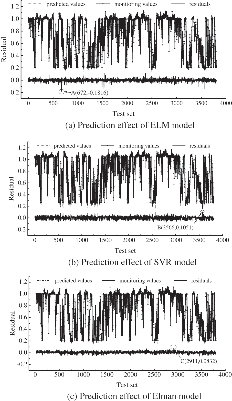
Figure 5: Prediction effect of single model

As shown in Fig. 5, each single model’s spindle speed monitoring value basically overlaps with the predicted value, with the predicted value minus the actual monitoring value as the residual value, where the residual maximum of ELM model in Fig. 5a is −0.1816, that is, A (672, −0.1816), the residual maximum of SVR model in Fig. 5b is 0.1051, namely B (3566, 0.1051), the residual maximum of Elman model in Fig. 5c is 0.0832, which is C (2911, 0.0832), and the residual maximum of each single model The mean values of residuals are −0.0002, 0.0021, and 0.0062, correspondingly.

(3) The entropy value methodology was employed to determine the weights of the single prediction models in the combined prediction model, and the predictive efficiency of the combined model as shown in Fig. 6.

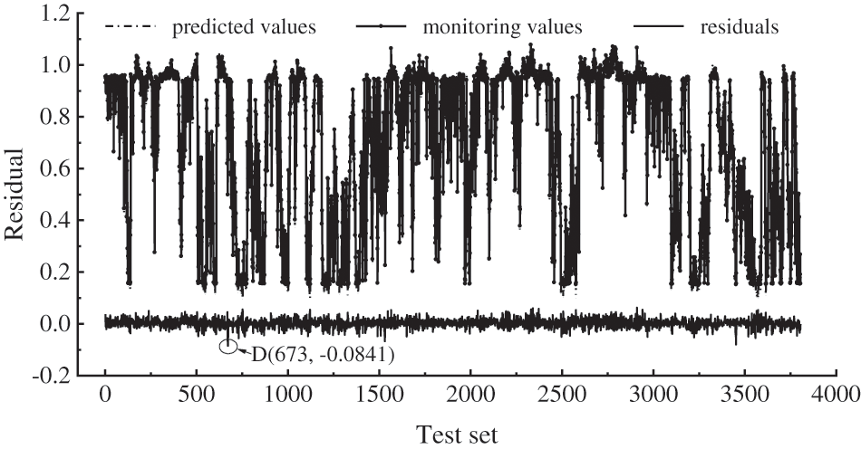
Figure 6: Prediction effect of combined model

As can be seen from Fig. 6, the residual value of the combination model has a maximum of −0.0841 at point D, namely D (673, −0.0841), with a mean residual value of 0.0027, in which the maximum value of the residual of the combined model is 0.0974 and 0.0765 respectively less than the maximum value of the residual of the ELM and SVR single models, while compared with the Elman single model increased by 0.0009. In addition, as the mean value of residuals increased by 0.0025 and 0.0006 when compared with ELM and SVR model, whereas the mean value of residuals decreased by 0.0035 compared with Elman model, hence the optimal model is not evaluated by the maximum value of residuals and the mean value of residuals, and the prediction accuracy of each model needs to be further verified.

(4) Adopting the evaluation indexes MAPE, RMSE, MAE and R2 to evaluate the models, with the comparison of the evaluation indexes of each model shown in Table 6.

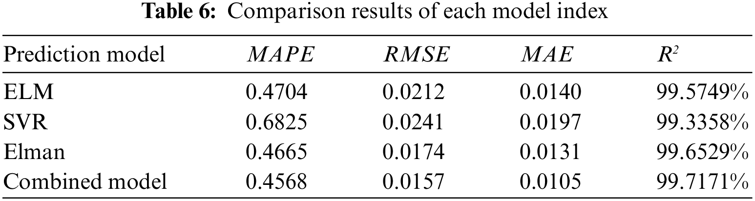
As shown in Table 6, the combined model is optimum compared with the single model of ELM, SVR and Elman. Where MAPE is reduced by 0.0136, 0.2257, and 0.0097, depending on each single model. RMSE is respectively decreased by 0.0055, 0.0084 and 0.0017 compared with the single model. MAE is separately reduced with the single model by 0.0035, 0.0092 and 0.0026. R2 improved by 0.1422%, 0.3813% and 0.0642%, compared with the singular model.

(5) The combination model is determined as the optimal prediction model.

5.2 Identification of Spindle Running State

Set the sliding window width N as 10, increment q as 1 to calculate C(N), and then take α as 0.05, according to the small probability principle, the confidence level is 99.95%, based on Eq. (13) to calculate Cth as 0.5660. The SCADA monitoring data of the unit for 10 days before the occurrence of fault is selected as the abnormal condition test data, and the SCADA monitoring data of the unit for 10 days of normal operation is selected as the normal condition test data. After normalizing the test data into the combined model for prediction, when C(N) is continuously above the threshold value of 0.5660 for three or more times, it is judged as an abnormal state. The identification results of the spindle speed operation state index during the spindle operation of the unit are shown in Fig. 7.

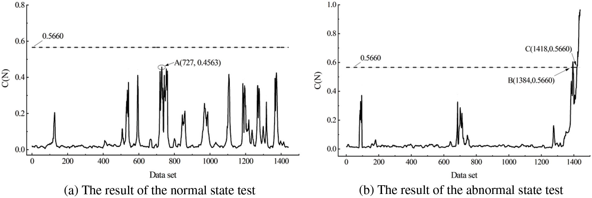
Figure 7: The result of spindle speed operation state index identification

As shown in Fig. 7a, the spindle speed operation status index of this set is 0.4563 at the maximum value within the normal state test data set, and the whole are below the threshold value of 0.5660, so that the spindle confined in the normal operation state. In Fig. 7b, the results obtained from the abnormal state test data set containing the spindle fault data of the wind turbine are illustrated. The spindle speed operation state index of the wind turbine continuously breaks the threshold value and emits an early warning at the 1384th data point of the data set, and later breaks the threshold value and continues to be higher than the threshold value at the 1418th data point, in which the spindle of the wind turbine fails and is consistent with the actual fault data, It indicates that the failure alert time of the monitoring method in this work is 5.7 h earlier than the actual failure occurrence time, which can achieve the purpose of identifying and alerting the abnormal state of wind turbine spindle operation.

6  Conclusions

In order to address the difficulty of collecting fault data from in-service wind turbine SCADA system, this work proposed a research approach for wind turbine spindle operation status driven entirely by SCADA normal data. At first, the QM-DBSCAN process is employed to clean the SCADA raw data and extract the feature parameters with the spindle speed as the output parameter. The next, ELM, SVR, Elman and combined prediction models were constructed based on the R language platform, and the combined prediction model was obtained as optimal with evaluation indexes MAPE, RMSE, MAE and R2, whereby MAPE was reduced by 0.0136, 0.2257 and 0.0097 compared with each single model. RMSE was reduced by 0.0055, 0.0084 and 0.0017, correspondingly. MAE decreased respectively by 0.0035, 0.0092 and 0.0026. R2 increased separately by 0.1422%, 0.3813% and 0.0642% from the single model. At the last, the spindle operation status early warning threshold is computed and verified with actual SCADA data based on the assumption of small probability events. Such system can detect potential failures and alert in advance, which has implications for wind turbine spindle running condition recognition and maintenance.

Funding Statement: This work was supported by the National Natural Science Foundation of China (No. 51965034).

Conflicts of Interest: The authors declare that they have no conflicts of interest to report regarding the present study.

References

    1. Zhao, H. S., Liu, H. H. (2018). Condition analysis of wind turbine main bearing based on deep belief network with improved performance. Electric Power Automation Equipment, 38(2), 44–49. [Google Scholar]

    2. Li, G., Qi, Y., Li, Y. Q., Zhang, J. F., Zhang, L. H. (2021). Research progress on fault diagnosis and state prediction of wind turbine. Automation of Electric Power Systems, 45(4), 180–191. [Google Scholar]

    3. Hossain, M. L., Abu-Siada, A., Muyeen, S. M. (2018). Methods for advanced wind turbine condition monitoring and early diagnosis: A literature review. Energies, 11(5), 1–14. DOI 10.3390/en11051309. [Google Scholar] [CrossRef]

    4. Feng, Z. P., Zhou, Y. K., Zuo, M. J., Chu, F. L., Chen, X. W. (2017). Atomic decomposition and sparse representation for complex signal analysis in machinery fault diagnosis: A review with examples. Measurement, 103(1), 106–132. DOI 10.1016/j.measurement.2017.02.031. [Google Scholar] [CrossRef]

    5. Malik, H., Almutairi, A. (2021). Modified Fuzzy-Q-Learning (MFQL)-based mechanical fault diagnosis for direct-drive wind turbines using electrical signals. IEEE Access, 9(1), 52569–52579. DOI 10.1109/ACCESS.2021.3070483. [Google Scholar] [CrossRef]

    6. Elasha, F., Shanbr, S., Li, X. C., Mba, D. (2019). Prognosis of a wind turbine gearbox bearing using supervised machine learning. Sensors, 19(14), 3092–3109. DOI 10.3390/s19143092. [Google Scholar] [CrossRef]

    7. Guo, Y., Zhao, Z., Sun, R., Chen, X. (2021). Data-driven multiscale sparse representation for bearing fault diagnosis in wind turbine. Wind Energy, 22(4), 587–604. DOI 10.1002/we.2309. [Google Scholar] [CrossRef]

    8. Yang, S. J., Yang, P. K., Yu, H., Bai, J., Feng, W. W. et al. (2022). A 2DCNN-RF model for offshore wind turbine high-speed bearing-fault diagnosis under noisy environment. Energies, 15(9), 3340. DOI 10.3390/en15093340. [Google Scholar] [CrossRef]

    9. Shahriar, M. R., Borghesani, P., Ledwich, G., Tan, A. (2018). Performance analysis of electrical signature analysis-based diagnostics using an electromechanical model of wind turbine. Renewable Energy, 116(B), 15–41. DOI 10.1016/j.renene.2017.04.006. [Google Scholar] [CrossRef]

  10. Jin, X. H., Peng, Y. Y., Cheng, F. Z., Qiao, W., Qu, L. Y. (2016). Quantitative evaluation of wind turbine faults under variable operational conditions. IEEE Transactions on Industry Applications, 52(3), 2061–2069. DOI 10.1109/TIA.2016.2519412. [Google Scholar] [CrossRef]

  11. Liu, X. C., Du, J. A., Ye, Z. S. (2021). A condition monitoring and fault isolation system for wind turbine based on SCADA data. IEEE Transactions on Industrial Informatics, 18(2), 986–995. DOI 10.1109/TII.2021.3075239. [Google Scholar] [CrossRef]

  12. Jia, X. J., Han, Y., Li, Y. J., Sang, Y. C., Zhang, G. L. (2021). Condition monitoring and performance forecasting of wind turbines based on denoising autoencoder and novel convolutional neural networks. Energy Reports, 23(7), 6354–6365. [Google Scholar]

  13. Senanayaka, J., Kandukuri, S. T., Khang, H. V. (2017). Early detection and classification of bearing faults using support vector machine algorithm. IEEE Workshop on Electrical Machines Design, Control and Diagnosis, Nottingham. [Google Scholar]

  14. Hu, L. Y., Jiang, W. B., Li, Y. T. (2021). Fault diagnosis for wind turbine based on LightGBM. Acta Energiae Solaris Sinica, 42(11), 225–259. [Google Scholar]

  15. Adnan, R. M., Mostafa, R. R., Kisi, O., Yaseen, Z. M., Shahid, S. et al. (2021). Improving streamflow prediction using a new hybrid ELM model combined with hybrid particle swarm optimization and grey wolf optimization. Knowledge-Based Systems, 230(27), 1–19. DOI 10.1016/j.knosys.2021.107379. [Google Scholar] [CrossRef]

  16. Xiao, C., Liu, Z. J., Zhang, T. L., Zhang, L. (2019). On fault prediction for wind turbine pitch system using radar chart and support vector machine approach. Energies, 12(14), 1–18. DOI 10.3390/en12142693. [Google Scholar] [CrossRef]

  17. Ma, X. Y., Zhang, X. H. (2022). A short-term prediction model to forecast power of photovoltaic based on MFA-Elman. Energy Reports, 8(4), 495–507. DOI 10.1016/j.egyr.2022.01.213. [Google Scholar] [CrossRef]

  18. Waseem, M., Ajmal, M., Kim, T. W. (2015). Development of a new composite drought index for multivariate drought assessment. Journal of Hydrology, 527(1), 30–37. DOI 10.1016/j.jhydrol.2015.04.044. [Google Scholar] [CrossRef]

  19. Zhang, F., Liu, D. S., Dai, J. C. (2019). An operating condition recognition method of wind turbine based on SCADA parameter relations. Journal of Mechanical Engineering, 55(4), 1–9. DOI 10.3901/JME.2019.04.001. [Google Scholar] [CrossRef]