Improving Performance of Recurrent Neural Networks Using Simulated Annealing for Vertical Wind Speed Estimation

Nomenclature

1  Introduction

Wind power plants have been used globally as a renewable energy source for household and industrial energy demand. Total deployed wind power capacity, worldwide in 2020 cumulatively, reached 743 GW [1], and more wind power plants are being planned to be installed to meet the demand and to combat the greenhouse gases (GHG) emissions, globally. However, wind power plant installation requires accurate and precise data on the availability and changes in wind speed (WS) of any site since WS may vary rapidly and increase with height as shown in Fig. 1 where WS at180 m is higher than that at 140 to 20 m. Therefore, more energy can be harvested if the hub height of the turbine is high. Today’s modern wind turbines have a rotor diameter of 120 m or more with a hub height of 100 m or more where the investment and installation costs are in proportion with the dimension. This indicates that an accurate estimation of the wind profile is needed at the turbine hub height for accurate estimation of the energy that can be generated from the turbine to be installed and prevents failure to achieve return of investment due to inaccurate wind profile investigation.

Figure 1: Measured wind speeds at 20, 60, 100, 140, and 180 m

The increase in WS with height is due to less human activities and lower surface roughness at higher heights. In addition, atmospheric conditions at a higher height have less friction and are more stable which may account for higher WS at higher heights [2]. However, in most countries, WS is measured at lower heights from 10 to 40 m. Therefore, for accurate estimation of wind power potential in an area for turbine positions above 40 m, WS must be estimated for higher turbine hub heights using physical, statistical, or machine learning intelligence techniques.

Several approaches have been used to estimate WS at higher positions based on measurements at lower heights as indicated by increasing WS average and its percentage increment in Fig. 2. Under stable atmospheric conditions, logarithmic approaches and power-law techniques for WS estimation have shown good accuracy [3]. Parametric approaches require fields survey to obtain meteorological coefficients as reported by Banuelos-Ruedas et al. [4] that used Hellman’s law, 1/7th power law, and a logarithmic approach to estimate WS at a given altitude. In addition to parametric methods, artificial intelligence (AI) approaches have been widely used for the temporal prediction of WS [5,6] due to its practicality. For example, Islam et al. [7] proposed a hybrid artificial neural network for WS estimation up to 100 m using measurements at the height of 10–40 m. Türkan et al. [8] compared seven different AI techniques for vertical WS estimation at a height up to 30 m using a WS measured at a height of 10 m. Emeksiz [9] developed multigene genetic programming for the temporal estimation of WS at different altitudes. Mohandes et al. [10] employed the Restricted Boltzmann Machine (RBM) technique to pre-train the neural network to estimate WS up to 120 m height using WS measurements at lower altitudes. Ti et al. [11] proposed artificial neural networks (ANN) based wake model to predict power produced by a wind farm. Wake modelling was also combined with the bilateral convolutional neural networks for dynamic wind farm power prediction [12]. Yang et al [13] developed double layer machine learning framework using ANN and Bayesian machine learning for wind farm power prediction. It can be noticed that the modern and advanced AI approaches have been widely investigated for temporal WS estimation, but limited number of works are used for vertical WS estimation tasks using WS measured at lower heights. Therefore, the literature above has shown the necessity for the investigation of a hybrid AI method for WS estimation above 120 m.

Figure 2: Wind speed average and its corresponding percentage increment

The contributions and novelties of this study are as follows:

1.    The paper introduces two steps performance enhancement of recurrent neural networks using gradient based and simulated annealing methods to estimate WS at a higher turbine position using the measured value at lower heights.

2.    This paper presents the comparison of the proposed method with the standard RNN, Multilayer Perceptron (MLP), Support Vector Machine (SVM), and state of the art methods like convolutional neural networks (CNN) and long short-term memory methods.

3.    A real dataset from Dhahran, Kingdom of Saudi Arabia is used to evaluate the accuracy of the proposed method.

4.    All methods are evaluated using error metrics such as mean squared error (MSE), mean absolute percentage error (MAPE), mean bias error (MBE), and coefficient of determination (R2).

The remainder of this paper is structured as methodology, experimental results, and conclusion.

2  Methodology

2.1 Proposed Method and Its Mathematical Models

In this paper, we propose a hybrid method, namely recurrent neural networks with simulated annealing (RNN-SA) for vertical WS extrapolation. The RNN uses the Elman model where the hidden unit output is connected back to itself using an adjustable recurrent weight (w)in addition to feeding the output layer with weights (V), as shown in Fig. 3. Although the architecture is simple, this model is capable of performing a variety of prediction tasks [14,15]. The data is pre-processed in two stages. First, the data from the input (U) and recurrent connections are provided to the hidden units as inputs. Next, the output from the hidden units is sent to both the output layer and through the recurrent connections back to the hidden units. Mathematically, the output of the kth hidden unit hk(n) given the nth input vector is given by:

Figure 3: RNN with Elman model for WS extrapolation

hk(n)=σ(Ukx(n)+Wkhk(n−1)+bk)(1)

where b is the bias vector. The input x represents the actual and estimated WS from the lower heights. The output layer provides the WS value at one step higher. The output y(n) of the nth sample is given by:

y(n)=σ(Vh(n)+by)(2)

This study uses the tangent-hyperbolic activation function defined by:

σ(z)=ez−e−zez+e−z(3)

In this study, the numerical experiment is carried out by dividing the data into three parts, i.e., 70%, 10%, and 20% for training, validation, and testing, respectively. The RNN-SA is trained using the Broyden-Fletcher-Goldfarb-Shanno (BFGS) algorithm [16]. Since the model uses a medium number of units and layers, the BFGS algorithm is the most suitable for unconstrained optimization [17]. The BFGS algorithm is utilized to obtain the RNN model with minimum mean squared error (MSE):

E=MSE=∑n=1N(yn−y^n)2N(4)

It can be noticed that the MSE is a continuously differentiable function that represents the difference between the predicted outputs (y^) and the actual values (y). The BFGS algorithm uses an iterative update to obtain the weights that minimize the cost function e(w)=E from Eq. (4). The weight update is specified by:

wk+1=wk+μkdk(5)

where μk and dk denote the step size and direction at iteration k. The direction update is given by:

{dk=−Bk−1∇e(wk)Bk+1=Bk−BkskskTBkSkTBksk+ykykTykTsk,B0=Isk=wk+1−wk,yk=∇e(wk+1)−∇e(wk)(6)

where Bk is an approximation of the Hessian matrix that represent the second derivative of the cost function. The results of the validation data showed that the RNN method with L=20 hidden units and number of iterations, K=20, exhibited the best performance. The model is further optimized using simulated annealing (SA), which is an optimization method that accepts not only better solution candidates but also includes not so good ones with a certain likelihood to enable the optimization to explore a new area for new candidates [18]. In the sense of the RNN, the SA is utilized further to optimize the trained RNN with respect to a non-differentiable cost function, namely, the mean absolute error (MAE):

MAE=1N∑n=1N|yn−y^n|×100%(7)

Given the cost function above, the solution candidate acceptance is given by:

p=11+eΔEmax(T)(8)

where ΔE is the difference between new and old cost functions and T is the temperature governed by the following relation:

T=T0×0.95k(9)

where the initial temperature T0 is set to 100 and k is the iteration number. The proposed RNN-SA utilizes two-stage optimizations. First, the BFGS method trains the RNN to minimize the MSE. The first cost function uses a smooth quadratic function that allows gradient-based optimization to obtain the best solution. Second, the SA optimizes the trained RNN weights to achieve the minimum MAE. Since the MAE uses a non-smooth absolute function, the SA offers an optimal solution for a complex recurrent model. The proposed two steps optimization approach to improve the performance metrics with different methods namely, the MSE with continuous derivative and the non-smooth MAE. The traditional RNN is typically trained using gradient based method with differentiable cost function. Whereas, the proposed RNN, in addition to the gradient based method, is further optimized using SA to enhance the performance. Both RNNs use the same architecture with recurrent units as shown in Fig. 4. In the implementation, the maximum number of iterations of the SA method is K=10.

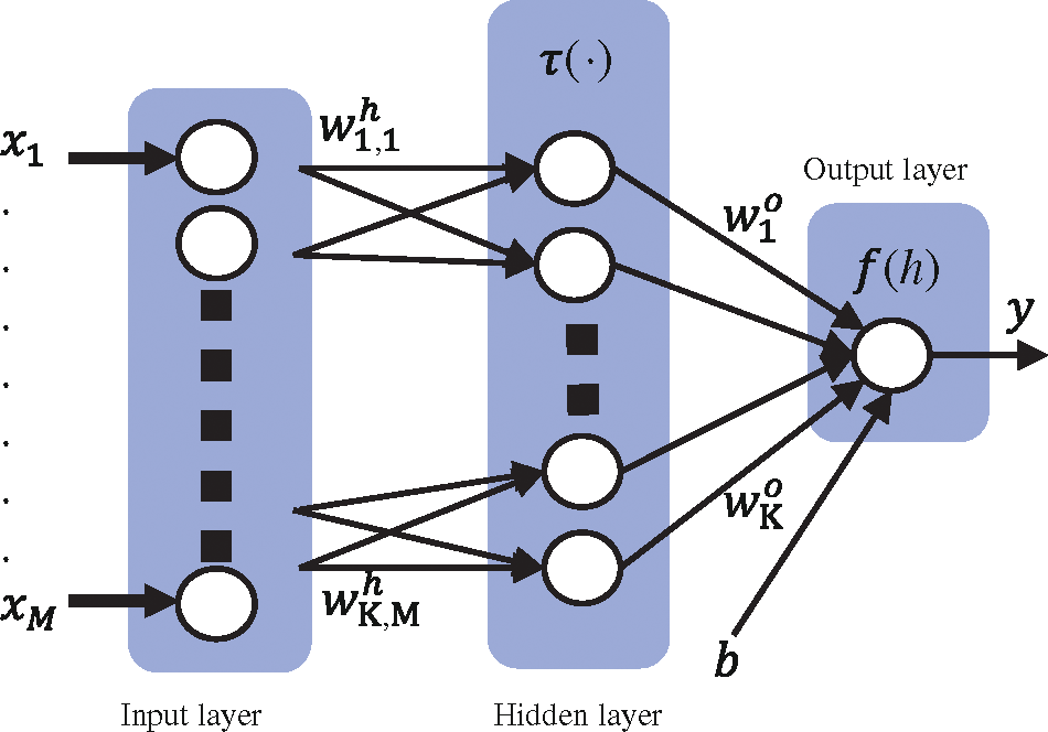
Figure 4: Multi-layer perceptron model

2.2 Multilayer Perceptron

In this study, the multilayer perceptron (MLP) is used as a benchmark for the comparison of the performance of RNN-SA. MLP has a much simpler structure than RNN [19], as shown in Fig. 4. In contrast to RNN, MLP uses a feed-forward structure that sequentially processes the data from the input layer to the output layer. Mathematically, the output of the kth hidden unit hk(n) given the nth input vector is obtained by:

hk(n)=τ(Whx(n)+bk)(10)

where Vk is the input weight matrix. Given the hidden unit values, the output of the MLP is defined by:

y(n)=Woh(n)+b(11)

This study utilizes gradient descent with momentum and adaptive learning rate (μ) backpropagation to train the MLP. This method is able to train any model with differentiable activation and cost function, which is suitable in this case where the activation and cost function uses differentiable tangent hyperbolic and MSE, respectively. Each weight is adjusted according to gradient descent defined by:

wk=wk−1+∂wk(12)

where the weight update (∂wn) is calculated by:

∂wk=m∂wk−1+mμ(∂ek)∂wk(13)

where m=0.9 and μ=0.01 denote the momentum coefficient and learning rate, respectively [20]. The cost function is evaluated at each epoch. If the cost function decreases toward the cost target, then the learning rate is increased by the factor Δμ(+)=1.05. If the cost function improves by more than the factor ΔMSEmax=1.04, the weight update that increased the cost function is canceled, and the learning rate is updated by the factor Δμ(−)=0.7. The experiments use H=20 hidden units. Training halts when the maximum number of iterations (K=1200) is exceeded.

2.3 Support Vector Machine

The last benchmarking method used in this paper is the support vector machine (SVM) for regression [21]. Theoretically, SVM is represented by a mapping function {(xi,yi)}i=1N, with input vectors xi∈RM and output targets yi∈R. The SVM attempts to create the relationship between xi and expected results f(xi) as follows:

y=f(xi)=(ω⋅xi)+b(14)

where ω∈RM and b are the weight vectors and threshold, respectively. From this model, the target of SVM is to obtain the weights that minimize the following error function:

E(ω)=1N∑i=1N|yi−f(xi)|ϵ+λ|ω|2(15)

where λ is a constant and the robust error function |z|ϵ is defined as follows:

|z|ϵ={0,if|z|<ϵ|z|,otherwise.(16)

The SVM model is trained using sequential minimal optimization (SMO), where the number of inputs determines the dimension of ω. Since the model has four input elements (10, 20, 30, and 40 m), the model for estimating WS at 50 m uses M=4.

2.4 State of the Art Methods

Recently, state of the art methods like deep learning have been used for many tasks including wind speed prediction. For instance, convolutional neural networks (CNN) is used for WS prediction in a wind farm in Hebei Province, China with high accuracy [22]. In addition to that, long short-term memory (LSTM) network is used for WS prediction on a wind farm in Inner Mongolia [23]. These two methods are also used as benchmarking methods in this paper.

2.5 Error Measures

This study employs four error measures based on the difference between the measured values (y), the estimated outputs (y^), and the average of the measured values (y¯), including MSE, mean bias error (MBE), mean absolute percent error (MAPE), and the coefficient of determination (R2). These error measures are calculated using the following equations:

MBE=∑n=1N(y^n−yn)N(17)

MAPE=1N∑n=1N|yn−y^nyn|×100%(18)

R2=(1−∑n=1N(yn−y¯)2∑n=1N(yn−y^n)2)×100%(19)

3  Numerical Experimental Results

This section provides the description of the experimental setup and the results. The estimation starts by training each model using WS values at heights 10, 20, 30, and 40 m, as inputs and actual WS at the height of 50 m as the target. Next, the actual WS at 10–40 m and the estimated WS at a height 50 m are used to train new model with five inputs to estimate the WS at 60 m height. This process, which uses the actual and estimated WS values at lower heights to predict the WS values at one level higher is further repeated until the estimation of the WS at a height of 180 m using the actual WS at 10–40 m, and the estimated WS at 50–170 m is obtained.

3.1 Wind Speed Dataset

Due to lack of resources in some countries, WS is typically measured up to a height of 40 m and its extrapolation to higher levels require sophisticated methods. Therefore, the WS at the higher heights is obtained using models, given the WS measured at lower heights. As shown in Fig. 1, the WS increases with height but in a random fashion [24,25]. This paper uses WS data acquired in Dhahran, Saudi Arabia during 20 June 2015 to 29 February 2016 using a LiDAR wind measurement device at 10, 20, 30, …, 180 m heights. The WS is scanned every three second and averages at each 10 min are saved and used. The data is divided into training, validation, and testing at 70%, 10%, and 20%, respectively. The LiDAR based measured WS is used as the reference for the actual WS.

3.2 Results

Table 1 shows the performance of the RNN-SA under validation data for WS estimation at 50–180 m heights based on measured WS at 10–40 m heights. The model with the best performance is further used for testing. Table 2 summarizes the testing data experimental results of the RNN-SA, standard RNN, MLP, SVM, CNN, and LSTM techniques in terms of MSE. It is obvious that MSE values for RNN-SA increases progressively from 0.027 to 2.089 while that for MLP from 0.049 to 2.367, corresponding to 50 to 180 m heights. Similarly, for the SVM method, the MSE values varied from 0.032 at 50 to 2.632 at 180 m. In all the numerical experiments, that RNN-SA method resulted in lowest values of MSE at all heights. The developed method is able to achieve better MSE than the standard RNN for all heights. It also can be noticed that the RNN-SA outperformed other methods based on the obtained MSE values. Table 3 reports the MBE of all methods and heights. MBE may not quantify the performance or accuracy of the estimation methods; however, it indicates whether the method is over or under predictive [26]. Positive MBE represents over prediction where the estimated values are larger than the actual one. Whereas, negative MBE indicates under-prediction where the estimated values are less than the actual. The experimental results show that all methods have negative values for all the heights. This indicate that the predicted values are less than the measured WS or the model underestimated the WS at all heights.

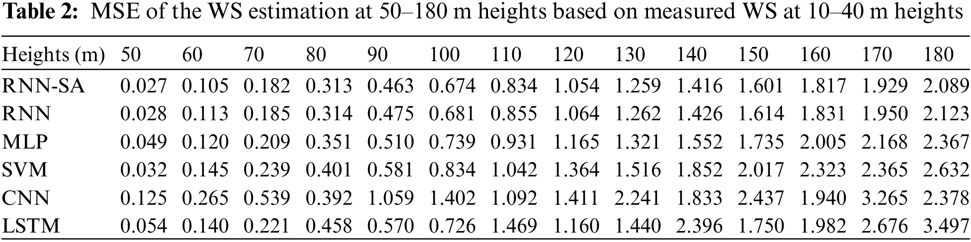
Fig. 5 compares the MAPE values for all the methods and show almost the same pattern as in case of MSE (Table 1). The MAPE value of RNN-SA, standard RNN, MLP, and SVM increased from 2.2% to 11.2%, 2.3% to 11.3%, 2.9% to 11.7%, and 2.4% to 12.2% for 50 to 180 m of heights, respectively. The proposed method achieves the least MAPE over all methods for all the heights. RNN methods proved to be the next best estimator of WS at all heights while MLP the third best option. Fig. 6 visualizes the R2 values for all heights and methods. The figure shows that the estimated values deviate more and more from the actual values as height increases. It may be accounted to the fact that actual WS values at 10–40 m only are being used for the estimation at higher heights. So, the estimated WS near the 40 m height has higher accuracy, and as the height increases, the correlation between the estimated and the actual WS decreases. The RNN-SA outperforms the other methods and achieved the highest R2 values for all heights.

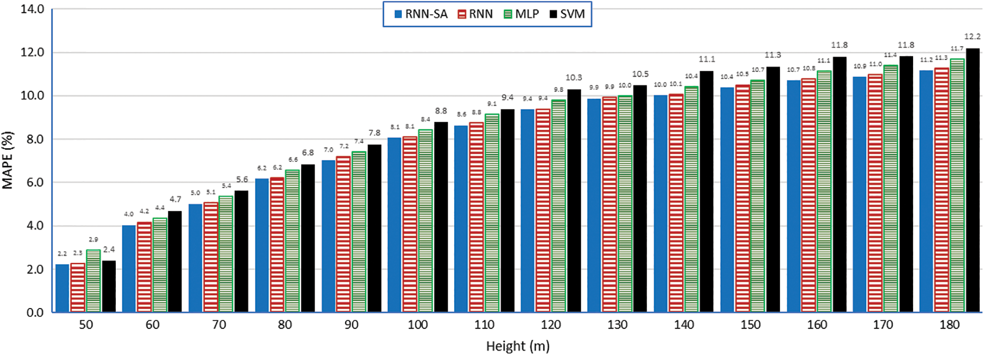
Figure 5: MAPE of different methods and all heights

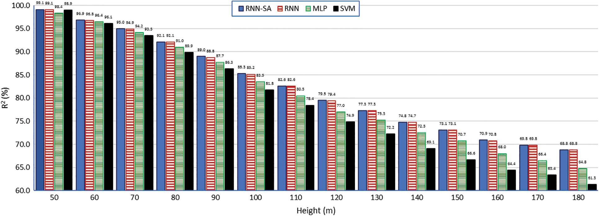
Figure 6: R2 of different methods and all heights

The scatter plots between the estimated RNN-SA with actual WS values at 60, 100, 140, and180 m are shown in Figs. 7a–7d, respectively. It is observed that the scatter plots start to diverge as height increases. This is confirmed by the temporal variation of actual and extrapolated WS values at 60, 100, 140, and 180 m heights, shown in Figs. 8a–8d, respectively. It is noticed that the estimated WS values follow the temporal trend of actual values at all heights, as depicted in Fig. 8. The figure also shows the coefficient of determination values for all methods. However, the trends of estimated WS at 180 (Fig. 8d) m are away from the actual values compared to the trends at 60 m (Fig. 8a), 100 m (Fig. 8b), and 140 m (Fig. 8c). The maximum number of estimated WS values for training contribute to these deviations.

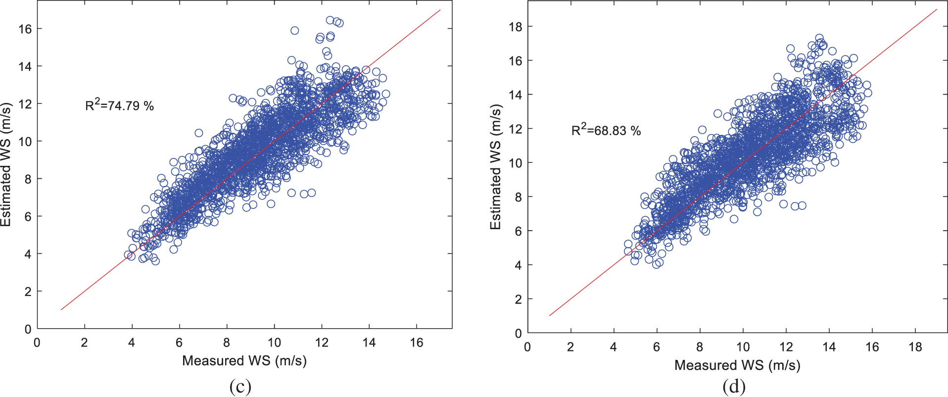
Figure 7: Scatter plots actual and estimated WS using the proposed method at 60, 100, 140, and 180 m

Figure 8: Wind profile of measured and estimated WS at (a) 60, (b) 100, (c) 140, and (d) 180 m

The estimated WS profiles along with the actual ones up to 180 m, are compared in Fig. 9. Each line in Figs. 9a–9e represents an individual WS value at a particular time sample. It is evident from the figure that the estimated WSs at lower heights are very close to the actual values. In contrast, the estimated WS higher heights tend to deviate from the actual. Fig. 9f represents the average of WS for all time samples. The average estimated WS for all methods confirm the observation in Table 2, where the average of estimated WS is less than the actual one.

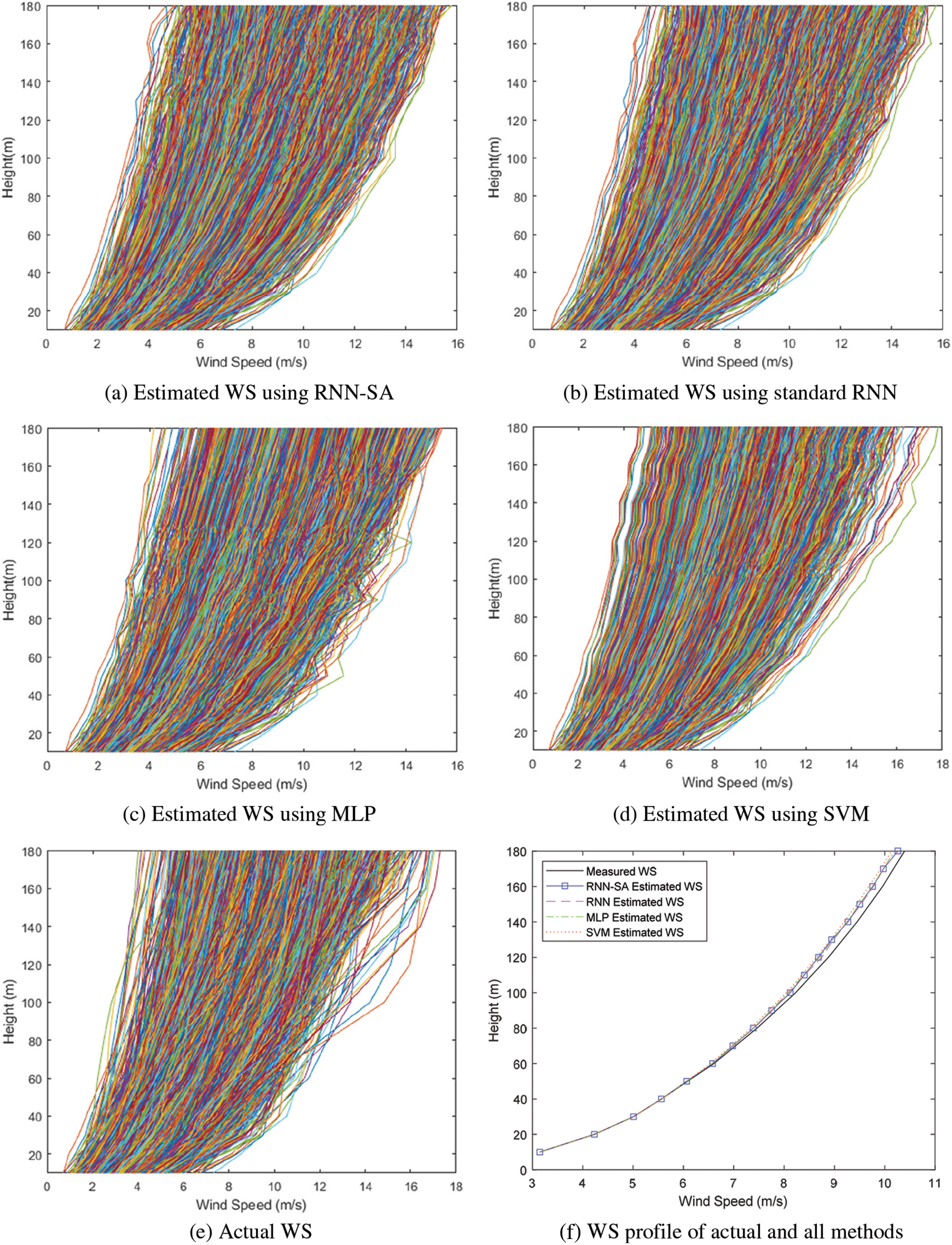
Figure 9: Wind profile of actual and estimated for all heights

Finally, the training duration statistics is shown in Fig. 10. It can be noticed that the proposed training method takes a bit more extra training time as indicated by higher training duration. Maximum training duration of the proposed and traditional RNN approaches are 47.77 and 36.94 s, respectively. Despite the relative high difference of the maximum duration (10.8 s), the average training duration of the proposed and traditional RNN methods are 32.39 and 31.62 s, respectively. In other words, the additional step consumes a relatively small-time duration since the average training time difference is only 0.77 s. The extra training duration is compensated by the performance improvement, as shown by the data in Tables 2 and 3.

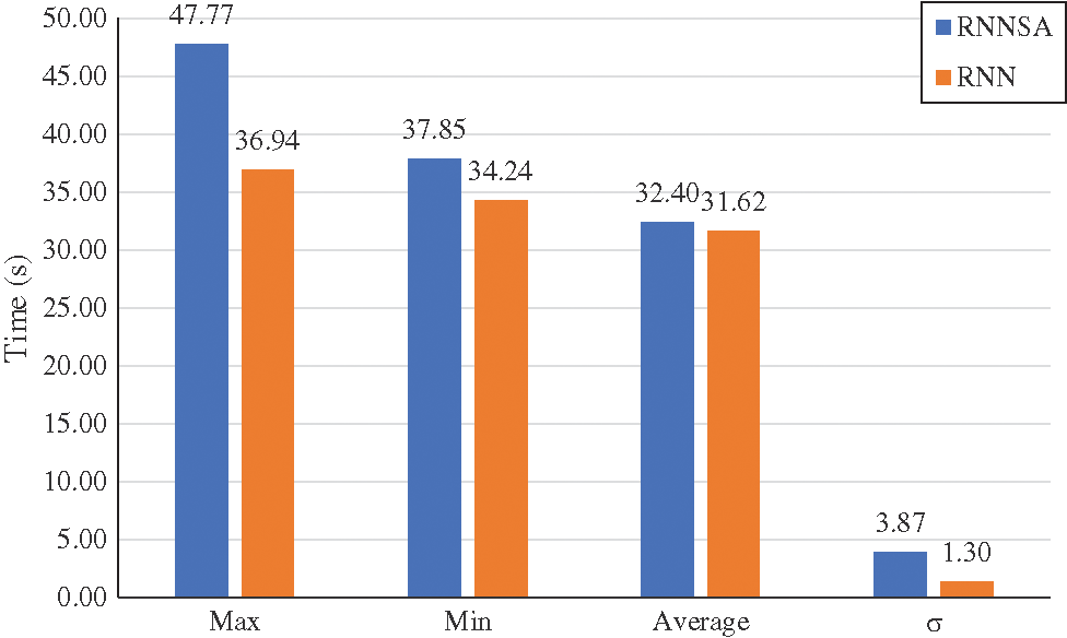
Figure 10: Training duration

4  Conclusions

This paper introduced a novel optimization method for the RNN using simulated annealing for accurate vertical WS extrapolation tasks. Each model is trained using the actual WS at lower heights (10–40 m) to estimate the WS up to 180 m. The novel method outperformed the standard RNN as well as other methods and state of the art models for all error measures on a real WS dataset. The novel method achieved the highest coefficient of determination (R2) values of 96.88%, 82.25%, 74.79%, and 68.83% between the estimated and the actual WS values at 60, 100, 140, and 180 m, respectively. Similarly, the other error matric measures MAPE and MSE showed the lowest values of error between the measured and estimated wind speeds at all the heights. The proposed novel method is recommended for wind speed extrapolation to higher heights using the available measurements at lower heights.

Funding Statement: This research was funded by KFUPM under Grant No. DF191024.

Availability of Data and Materials: The program is written using Matlab and is available at (https://github.com/hilalnuha/RNNverticalWS).

Conflicts of Interest: The authors declare that they have no conflicts of interest to report regarding the present study.

References

1. GWEC (2020). Global Wind Report 2021—Annual Market Update (Gwec-2021). https://gwec.net/global-wind-report-2021/. [Google Scholar]
2. Högström, U., Smedman, A. S., Bergström, H. (2006). Calculation of wind speed variation with height over the sea. Wind Engineering, 30(4), 269–286. DOI 10.1260/030952406779295480. [Google Scholar] [CrossRef]
3. Newman, J. F., Klein, P. M. (2014). The impacts of atmospheric stability on the accuracy of wind speed extrapolation methods. Resources, 3(1), 81–105. DOI 10.3390/resources3010081. [Google Scholar] [CrossRef]
4. Banuelos-Ruedas, F., Angeles-Camacho, C., Rios-Marcuello, S. (2011). Methodologies used in the extrapolation of wind speed data at different heights and its impact on the wind energy resource assessment in a region. In: Wind farm—technical regulations, potential estimation and siting assessment, pp. 97–114. http://www.intechopen.com/. [Google Scholar]
5. Gupta, D., Kumar, V., Ayus, I., Vasudevan, M., Natarajan, N. (2021). Short-term prediction of wind power density using convolutional RNN-SA network. FME Transactions, 49(3), 653– 663. DOI 10.5937/fme2103653G. [Google Scholar] [CrossRef]
6. Mohandes, M., Rehman, S., Nuha, H., Islam, M. S., Schulze, F. H. (2021). Accuracy of wind speed predictability with heights using long short-term memory. FME Transactions, 49(4), 908–918. DOI 10.5937/fme2104908M 2021. [Google Scholar] [CrossRef]
7. Islam, M. S., Mohandes, M., Rehman, S. (2017). Vertical extrapolation of wind speed using artificial neural network hybrid system. Neural Computing Applications, 28(8), 2351–2361. DOI 10.1007/s00521-016-2373-x. [Google Scholar] [CrossRef]
8. Türkan, Y. S., Aydoğmuş, H. Y., Erdal, H. (2016). The prediction of the wind speed at different heights by machine learning methods. An International Journal of Optimization and Control: Theories & Applications, 6(2), 179–187. DOI 10.11121/Ijocta.01.2016.00315. [Google Scholar] [CrossRef]
9. Emeksiz, C. (2022). Multi-gen genetic programming based improved innovative model for extrapolation of wind data at high altitudes, case study: Turkey. Computers and Electrical Engineering, 100(1), 107966. DOI 10.1016/j.compeleceng.2022.107966. [Google Scholar] [CrossRef]
10. Mohandes, M. A., Rehman, S. (2018). Wind speed extrapolation using machine learning methods and LiDAR measurements. IEEE Access, 6, 77634–77642. DOI 10.1109/ACCESS.2018.2883677. [Google Scholar] [CrossRef]
11. Zilong, Ti, Deng, X. W., Zhang, M. (2021). Artificial neural networks based wake model for power prediction of wind farm. Renewable Energy, 172, 618–631. DOI 10.1016/j.renene.2021.03.030. [Google Scholar] [CrossRef]
12. Li, R., Zhang, J., Zhao, X. (2022). Dynamic wind farm wake modeling based on a bilateral convolutional neural network and high-fidelity les data. Energy, 258(8), 124845. DOI 10.1016/j.energy.2022.124845. [Google Scholar] [CrossRef]
13. Yang, S., Deng, X., Ti, Z., Yan, B., Yang, Q. (2022). Cooperative yaw control of wind farm using a double-layer machine learning framework. Renewable Energy, 193(5), 519–537. DOI 10.1016/j.renene.2022.04.104. [Google Scholar] [CrossRef]
14. Mohandes, M., Rehman, S., Nuha, H., Islam, M. S., Schulze, F. H. (2021). Accuracy of wind speed predictability with heights using recurrent neural networks. FME Transactions, 49(4), 908–918. DOI 10.5937/fme2104908M. [Google Scholar] [CrossRef]
15. Cao, Q., Ewing, B. T., Thompson, M. A. (2012). Forecasting wind speed with recurrent neural networks. European Journal of Operational Research, 221(1), 148–154. DOI 10.1016/j.ejor.2012.02.042. [Google Scholar] [CrossRef]
16. Fletcher, R. (2000). Practical methods of optimization. Second Edition. The Atrium, Southern Gate, Chichester, West Sussex PO 19 8SQ, England: John Wiley & Sons, Ltd. DOI 10.1002/9781118723203. [Google Scholar] [CrossRef]
17. Lv, J., Deng, S., Wan, Z. (2020). An efficient single-parameter scaling memoryless Broyden-Fletcher-Goldfarb-Shanno algorithm for solving large scale unconstrained optimization problems. IEEE Access, 8, 85664–85674. DOI 10.1109/ACCESS.2020.2992340. [Google Scholar] [CrossRef]
18. Da, Y., Xiurun, G. (2005). An improved PSO-based ANN with simulated annealing technique. Neurocomputing, 63, 527–533. DOI 10.1016/j.neucom.2004.07.002. [Google Scholar] [CrossRef]
19. MATHWORKS (2022). Gradient descent with momentum and adaptive learning rate backpropagation. https://www.mathworks.com/help/deeplearning/ref/traingdx.html. [Google Scholar]
20. Yu, C. C., Liu, B. D. (2002). A backpropagation algorithm with adaptive learning rate and momentum coefficient. Proceedings of the 2002 International Joint Conference on Neural Networks. IJCNN’02 (Cat. No. 02CH37290), vol. 2, pp. 1218–1223. IEEE. [Google Scholar]
21. Wang, X., Wen, J., Zhang, Y., Wang, Y. (2014). Real estate price forecasting based on SVM optimized by PSO. Optik, 125(3), 1439–1443. DOI 10.1016/j.ijleo.2013.09.017. [Google Scholar] [CrossRef]
22. Zhu, X., Liu, R., Chen, Y., Gao, X., Wang, Y. et al. (2021). Wind speed behaviors feather analysis and its utilization on wind speed prediction using 3D-CNN. Energy, 236(5), 121523. DOI 10.1016/j.energy.2021.121523. [Google Scholar] [CrossRef]
23. Hu, Y. L., Chen, L. (2018). A nonlinear hybrid wind speed forecasting model using LSTM network, hysteretic ELM and differential evolution algorithm. Energy Conversion and Management, 173(2), 123–142. DOI 10.1016/j.enconman.2018.07.070. [Google Scholar] [CrossRef]
24. Rehman, S., Al-Hadhrami, L. M., Alam, M. M., Meyer, J. P. (2013). Empirical correlation between hub height and local logarithmic law for different sizes of wind turbines. Sustainable Energy Technologies and Assessments, 4(3), 45–51. DOI 10.1016/j.seta.2013.09.003. [Google Scholar] [CrossRef]
25. Haby, J. (2022). Wind speed increasing with heights. https://www.theweatherprediction.com/habyhints3/749/. [Google Scholar]
26. Shrestha, R., Di, L. P., Eugene, G. Y., Kang, L., Shao, Y. Z. et al. (2017). Regression model to estimate flood impact on corn yield using MODIS NDVI and USDA cropland data layer. Journal of Integrative Agriculture, 16(2), 398–407. DOI 10.1016/S2095-3119(16)61502-2. [Google Scholar] [CrossRef]
Cite This Article
Copyright © 2023 The Author(s). Published by Tech Science Press.
This work is licensed under a Creative Commons Attribution 4.0 International License , which permits unrestricted use, distribution, and reproduction in any medium, provided the original work is properly cited.
Downloads
Citation Tools