Application of Hankel Dynamic Mode Decomposition for Wide Area Monitoring of Subsynchronous Resonance

Nomenclature

1  Introduction

The fast growth and application of doubly-fed induction generators (DFIGs) in series compensated systems have significantly increased the occurrence of subsynchronous resonance (SSR) [1]. Recent SSR events in south Texas of USA [2] and North China [3,4] indicated that the oscillation could be system-wide which involves complex interactions among grid components. It is thus of great importance to provide a wide area monitoring of SSR parameters, including the magnitude, frequency and damping. The data are crucial for replicating SSR events, identifying the sources of SSR [5] and supporting the design of countermeasures, e.g., feedback-linearized sliding mode controller [6], energy-shaping L2-gain controller [7], damping controller [8].

To date, two types of data have been considered for SSR parameter identification (SSRPI). One is the waveform data provided by the fault recorder. This type of data contains the complete information of the oscillation and thus can be easily utilized for SSRPI through various signal-processing algorithms, such as Prony [9] and the recursive least square (RLS) method [10]. Additionally, model decomposition-based techniques, such as the Hilbert-Huang transform [11] and variational mode decomposition (VMD) [12], can perform parameter identification decomposition after the time signals are decomposed into multifrequency mode components. Unfortunately, the fault recorder is locally stored, and whether it records the SSR data depends on the triggering mechanism. This deficiency imposes great challenges for wide area monitoring or system-wide analysis [13].

Another option is to take advantage of the synchrophasors provided by the wide area monitoring system (WAMS). Currently, phasor measurement units (PMUs) have been widely deployed in transmission networks [14], making the WAMS a promising platform for SSR monitoring. The main challenge here is that the synchrophasor only captures the fundamental phasors. As a result, the SSR components will appear as the spectral leakage components. Studies have been conducted to address this issue. The work in [15] demonstrated that it is possible to identify the SSR frequency from synchrophasors. Recently, some modal parameter extraction methods, e.g., classic Prony analysis, estimation of signal parameters via the rotational invariance technique (ESPRIT) and the matrix pencil method [16], have been developed to extract the SSO parameters. In addition, the recent study in [17] further proposed a DFT-based correction method to recover the SSR amplitude from spectral leakage components. An interpolated DFT (InpDFT)-based method was also proposed in [13] to achieve better identification accuracy through the consideration of damping parameters.

However, the DFT-based methods rely on a long data window to obtain better accuracy for estimating the SSR parameters and assume that these parameters are constant within the window. In practice, the SSR parameters are usually time-varying due to the stochastic nature of wind resources and the volatile operation conditions of the grid [3]. When a short window is used in DFT-based methods for analyzing nonstationary signals, the spectrum of the SSR component in the synchrophasors will be significantly affected by spectral leakage from the fundamental frequency phasors. In this way, large estimation errors are unavoidable.

Within this context, this paper proposes a signal analysis technique based on dynamic mode decomposition (DMD). DMD seeks a linear dynamic operator to best approximate the underlying dynamics of the system. Its performance has been found to be satisfactory in a wide variety of applications, including fluid communities [18], biomedical fields [19] and power system areas. As an example, the work in [20] successfully applied DMD for spatiotemporal PMU data to monitor low-frequency oscillations.

In this paper, we implemented the key parameter estimation of SSR by using the DMD method from the eigenvalues of Hankel matrices after the behavior of the synchrophasors under SSR is analyzed. The contributions of this paper include the following: (1) temporal synchrophasors with less data (less than 1 s) are used to construct two Hankel matrices, and the computational efficiency is improved. Note that only a single channel of measurement is required here. (2) The DMD method is performed on two Hankel matrices to estimate the parameters of SSR, and the number of dominant modes is automatically determined rather than predetermined; thus, the dynamic performance of SSR is captured well. (3) The proposed method is performed on simulation and field data, demonstrating the effectiveness of the proposed method.

The remainder of the paper is organized as follows. Section 2 analyzes the behavior of synchrophasors under SSR and defines the DMD problem to be solved. The Hankel-DMD method is explained in Section 3 for the identification of SSR components. Section 4 verifies the effectiveness of the proposed method by using simulation data and field data under dynamic and noisy conditions. A comparative study is also conducted to show the superiority of the proposed method.

2  Synchrophasor Model under SSR

This paper focuses on the SSR caused by the interaction between DFIGs and series-compensated systems. For such cases, all wind farms and the network are engaged in one SSR mode [3,4,21]. As a result, the current waveform data in the time domain under SSR can be expressed as

x(t)=A1cos⁡(2πf1t+ϕ1)+Aseαstcos⁡(2πfst+ϕs)(1)

where αs is the damping factor of SSR and (A1,f1,ϕ1) and (As,fs,ϕs) are amplitudes, frequencies and initial phases of the fundamental and SSR components, respectively. With a fixed sampling frequency fp, the signal x(t) in (1) is sampled as x(n), expressed as

x(n)=A1cos⁡(2πf1fpn+ϕ1)+Aseαsfpncos⁡(2πfsfpn+ϕs)(2)

Commonly, synchrophasors are obtained by applying a discrete Fourier transform (DFT) on x(n) within a rectangle window. The length of the window is Np=fp/f0, and f0 is the nominal frequency, i.e., 50 or 60 Hz. Based on the Euler equation and series summation, the DFT spectra at the pth sliding time window can be derived as

X(p,k)=X1+(p,k)+X1−(p,k)+Xs+(p,k)+Xs−(p,k)p=1,2,…,k=0,1,…,Np−1(3)

where (X1+(p,k),X1−(p,k)) and (Xs+(p,k),Xs−(p,k)) are the positive and negative spectra of the fundamental and SSR components, respectively, and k is the spectral bin number.

Let fp1=f1/fp=L1/Np, αps=αs/fp=α^ps/Np and fps=fs/fp=Ls/Np, where L1 and Ls are the normalized f1 and fs expressed in spectral bins, respectively, and α^ps is the normalized damping ratio α^s. We compute X1±(p,k) and Xs±(p,k) as

{X1+(p,k)=A1C1(L1−k)ej(2πpfp1+ϕ1)X1−(p,k)=A1C1∗(L1+k)e−j(2πpfp1+ϕ1)Xs+(p,k)=ASCs(Ls−k)ej(2πpfps−jrαps+ϕs)Xs−(p,k)=AsCs∗(Ls+k)e−j(2πpfps+jrαps+ϕs)(4)

with

{C1(s)=12Np×1−ej2πs1−e(j2πs/Np),Cs(s)=12Np×1−e(α^ps+j2πs)1−e(α^ps+j2πs)/Np,(5)

where (.)∗ is the conjugate transpose operator, C1 represents the spectral leakage on the synchrophasors, considering that there is a frequency deviation between f1 and f0, and Cs represents the spectral leakage factor of the SSR component on the synchrophasors. Since we can only obtain AsC1 from the measured synchrophasor data, Cs is the key parameter for estimating As.

At the pth data window, the synchrophasor Xp(p) in the PMUs is obtained as the 2nd spectral.

bin (i.e., k=1) of the spectrum X in (3), expressed as

Xp(p)=X1+(p,1)+X1−(p,1)+Xs+(p,1)+Xs−(p,1)(6)

Assuming that f1, fs and αs do not change significantly in a short time window, we regard C1(L1−1) and C1∗(L1+1) in (4) as constants at a certain f1 and regard Cs(Ls−1) and Cs∗(Ls+1) as constants at a certain αs and fs.

Generally, a series of Xp provided by the PMUs are transmitted to the main station with a certain reporting frequency fr(=1/Tr, where Tr is the reporting interval time), typically 50 or 100 Hz for 50 Hz systems. Then, the reported synchrophasor Xc is obtained by resampling Xp with the interval fpr=fr/fp as Xc(m)=[Xp(0),…,Xp(mfpr−1)],(m=0,1,…). Accordingly, Xc should be expressed by replacing the variable p in (6) with mfpr, as shown in (7):

Xc(m)=A1C1(L1−1)ej(ωr1m+ϕ1)+A1C1∗(L1+1)e−j(ωr1∗m+ϕ1)+AsCs(Ls−1)ej(ωrsm+ϕs)+AsCs∗(Ls+1)e−j(ωrs∗m+ϕs)(7)

with

ωr1=2πf1Tr,ωrs=2πfsTr−jαsTr(8)

where ωr1 and ωrs are the normalized radial frequencies of the fundamental and SSR components related to Tr, respectively.

By defining

{a1=A1C1(L1−1)ejϕ1,a2=A1C1∗(L1+1)e−jϕ1a3=AsCs(Ls−1)ejϕs,a4=AsCs(Ls+1)e−jϕs(9)

and

{λ1=ejωr1,λ2=λ1∗λ3=ejωrs,λ4=λ3∗(10)

we rewrite (7) as

Xc(m)=a1λ1m+a2λ2m+a3λ3m+a4λ4m,(11)

which denotes that Xc under SSR is a linear combination of four distinct modes, i.e., (λ1,λ2) from the fundamental component and (λ3,λ4) from the SSR component. Generally, there are q frequency components in (11), and we generalize (11) as

Xc(m)=a1λ1m+…+arλrm(12)

where r=2q. When SSR does not occur, r=2, while when SSR occurs, r=4, as shown in (11).

Eq. (12) indicates that the synchrophasors under SSR are a linear combination of four phasors rotating at different frequencies. The index λi thus can be approached by the Hankel-DMD method using a series of synchrophasors. Once λi is known, the frequency fs and damping of the SSR can be calculated according to (8) and (10). Finally, As is determined by (5). The details are given in the next section.

3  Synchrophasor Model under SSR

This section first presents a Hankel-DMD method in which two Hankel matrices are constructed to satisfy the requirement of applying DMD. Then, the equations to calculate the frequency, damping and amplitude of the SSR are analytically derived.

3.1 Hankel-Dynamic Mode Decomposition

One premise to perform DMD is that the rank of the measurement matrix needs to be no less than the number of the dominant modes [22,23]. In the case that the measurement matrix is a series of temporal synchrophasors, its rank would be one, which is insufficient for SSRPI [22]. To address this issue, the concept of Hankel matrices is used here. For the Nth measured synchrophasor Xc(N), its N time-shifting historic data (Xc(0),…,Xc(N−1)) are collected to construct two Hankel matrices H1 and H2 as follows:

H1=[Xc(0)Xc(1)…Xc(N−L−1)Xc(1)Xc(2)…Xc(N−L)…………Xc(L−1)Xc(L)…Xc(N−1)](13)

and

H2=[Xc(1)Xc(2)…Xc(N−L)Xc(2)Xc(3)…Xc(N−L+1)…………Xc(L)Xc(L+1)…Xc(N)](14)

where H1,H2∈CL×(N−L) with min(L,N−L)>r, and L is generally set smaller than N−L.

Actually, H1, stacked from overlapping elements between adjacent rows or adjacent columns with high coherence, has the property of a low-dimensional structure, as shown by the singular value (i.e., σi i = 1,2,…,r) curve of noise-free H1 in Fig. 1a, where the singular values are obtained by using singular value decomposition (SVD) on noise-free H1. The number of nonzero singular values depends on the number of dominant modes in H1 (or Xc). Note that Fig. 1a represents the noise-free condition. In practice, the noises in Xc would perturb small singular values in H1 and H2. In other words, the number of nonzero singular values could be more than that of the dominant mode in Xc, as shown in Fig. 1b. It is definite that H2 has the same property as H1.

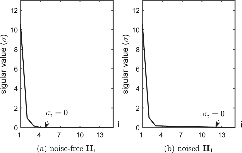
Figure 1: Singular value of H1 under the SSO component by using SVD. (a) Noise-free H1 and (b) noised H1

With the derivation in the Appendix, the relationship of H2 and H1 is determined as

H2=AH1(15)

where A∈CL×L is an unknown map from H1 to H2, given by

A=QΛQ†(16)

where ()† is the pseudo inverse of the matrix, and Q∈CL×r is given by

Q=[a1a2⋯ara1λ1a2λ2⋯arλra1λ12a2λ22⋯arλr2⋯⋯⋯⋯a1λ1L−1a2λ2L−1…arλrL−1]

and Λ∈Cr×r is given by

Λ=diag(λj),j=1,…,r(17)

where diag(.) constructs a diagonal matrix of λj in (11). Eqs. (16) and (17) imply that the frequency and damping of the SSR can be identified from the eigenvalues λj of the unknown map A. Since Hankel matrices H1 and H2 span the dominant modes of Xc, the unknown map A can be approached by computationally efficient DMD.

To reduce the impact of noise, reduced SVD is performed to seek the low-dimensional representation of H1. The SVD of H1 is given as

H1=UΣV*(18)

where U∈CL×L and V∈C(N−L)×L are the left and right singular vectors satisfying UU∗=I and VV∗=I, ∑∈CL×L is a diagonal matrix, i.e., Σ=diag(Σ1,…Σi,…ΣL), and Σi is the singular value of H1.

By retaining the first r columns of U and V, the reduced SVD gives a low-dimensional approximation of H1 as follows:

H1≈UrΣrVr∗(19)

where Ur=U(:,1:r), Σr=Σ(1:r,1:r), and Vr=V(:,1:r) in MATLAB notation. As shown in Fig. 1, in the noise-free case, Σr+1=…=ΣL=0 holds, whereas in the noisy case, Σr+1>…>ΣL>0 is caused by noise. Eq. (19) thus reduces the influence of noise.

The matrix Ur, as the proper orthogonal modes of H1, can project A into reduced dimensional space. Then, the reduced order model A¯∈Cr×r of A is given as

A¯≈Ur*AUr(20)

Since H2=AH1, A¯ can be determined by solving the optimization problem in (20):

minA¯‖H2−UrA¯ΣrVr*‖F(21)

where ‖⋅‖F is the Frobenius norm, and the least-square solution of (21) is given as

A=Ur∗H2VrΣr−1(22)

where (⋅)−1 is the inverse of the matrix. Note that the eigenvalues for A and A¯ are identical [20]; thus, an eigenvalue analysis of this matrix A¯ generates the eigenvalues and dynamic modes of the system.

3.2 Calculation of SSR Parameters

The modal parameters are obtained from the eigenvalues of A¯ by using eigenvalue decomposition as follows:

A¯=WΛW−1,(23)

where W∈Cr×r is the matrix of eigenvectors, and Λ is constructed by the eigenvalues λi, given in (17). Based on the relation between λi and (fi,αi) in (8) and (10), fi and αi can be determined as

fi=Imag(log⁡(λi))/(2π∗Tr)αi=Re(log⁡(λi))/Tri=1,2,…,r,(24)

where Imag(⋅) and Re(⋅) represent the imaginary and real parts of a complex number, respectively. In this paper, we consider that the frequency range of the SSR phasor is different from that of the fundamental phasor. Moreover, according to (10), a pair of conjugated frequencies come from fs. Based on the two rules, fs and λs of SSR can be determined.

Once λi is estimated, the amplitudes of SSR can be obtained by first solving αi in (12). Rewriting (12) in the matrix form gives

X¯c=Ea¯,(25)

with

a¯=[a1,a2,…,ar]T,X¯c=[Xc(0),Xc(1),…,Xc(N)]T,E=[11…1ejλ1ejλ2…ejλr…………ejλ1(N)ejλ2(N)…ejλr(N))](26)

where (⋅)T is the matrix transpose, and a¯ is solved in the least-square sense as follows:

a¯=(E∗E)−1E∗X¯c(27)

where (⋅)−1 is the inverse of the matrix.

Finally, the amplitude As of the SSR component is calculated according to (10):

As=|αs|/Cs(28)

where |⋅| is the absolute value, αs(1≤s≤r) corresponds to that of fs, and Cs is calculated by (5) with the obtained fs and αs.

3.3 Choice of Parameters

The proposed Hankel-DMD method provides a good dynamic performance, as it uses a very short data window for SSRPI. Under noise-free conditions, the proposed method can perform well as long as the dimensions of the constructed H1 and H2 satisfy min(L,N−L)≥r (r=4 in our problem). In practice, a longer data window is desired to reduce the impact of noise, but it also degrades the dynamic performance of DMD. Through sensitive studies using both simulation and field data, this paper suggests using N=50 or N=100 synchrophasors Xc, i.e., a 0.5 or 1 s data window for a 50 Hz system, and L is set to be L=N/3.

Another parameter that affects the performance of DMD is the selection of the number of dominant modes, i.e., r. Theoretically, r should be set as 2 when SSR does not occur and 4 after SSR occurs. The cumulative percentage sj of σi is used here to automatically determine the value of r, as shown in (29).

sj=∑i=1jσi∑i=1Jσi(29)

where J=min(L,N−L) and 1≤j≤J. Then, r is determined by a predefined threshold Th, given as

r=⌈j/2⌉×2,whensj≥Th,(30)

where ⌈⋅⌉ is the round up operator. Due to the impact of measurement noises, σi is not equal to zero when i>r. However, their eigenvalues are much smaller than those of the fundamental and SSR components. This indicates that j in (30) would be 1 or 2 when SSR does not occur and 3 or 4 after SSR occurs. Thus, (30) eliminates the impact of measurement noise and guarantees r to be 2 or 4 depending on the occurrence of SSR.

3.4 The Procedure of SSR Parameter Estimation

The whole procedure of the Hankel-DMD method to identify three key parameters of the SSR component, i.e., fs, αs and As, from the reported synchrophasors Xc can be summarized as follows:

•   Construct two Hankel matrices H1 and H2 by using (Xc(0),…,Xc(N−1),Xc(N)) according to (13) and (14);

•   Perform SVD of H1, i.e., H1=UΣV*, and determine r according to (30);

•   Calculate A¯ with Ur=U(:,1:r), Σr=Σ(1:r,1:r), and Vr=V(:,1:r) according to (22);

•   Perform eigen-decomposition of A¯ to obtain Λ=diag(λj);

•   Identify fs and αs according to (24);

•   Identify As according to (27) and (28).

4  Performance Tests

This section evaluates the performance of the proposed method using both simulations and field data. Comparative studies with the InpDFT method [13] and classical Prony method are also presented.

4.1 Synthetic Data

A synthetic SSR current data was constructed as (31), where an off-nominal frequency f1=49.7 Hz is considered

x(t)=1.0×cos⁡(2πf1t+π/2)+xs(t)(31)

The parameters of the SSR components, i.e., fs, αs and As, are set as

{xs(t)=0t∈[0,2)xs(t)=0.2×e0.08tcos⁡(2π×35.2t+π/6)t∈[2,4)xs(t)=0.35×e−0.1tcos⁡(2π×34.5t+π/3)t∈[4,10](32)

Fig. 2a shows the waveform of i(t) with a sampling rate of 10 kHz. It can be seen that SSR starts at t=2s and its modal parameters change at t=4s. The DFT algorithm was first performed on x(t) with Np=200 (i.e., one cycle) to obtain synchrophasors Xp, and then the reported synchrophasors Xc were generated by resampling Xp with reporting frequency fr=100 Hz. Fig. 2b shows the magnitude of Xc.

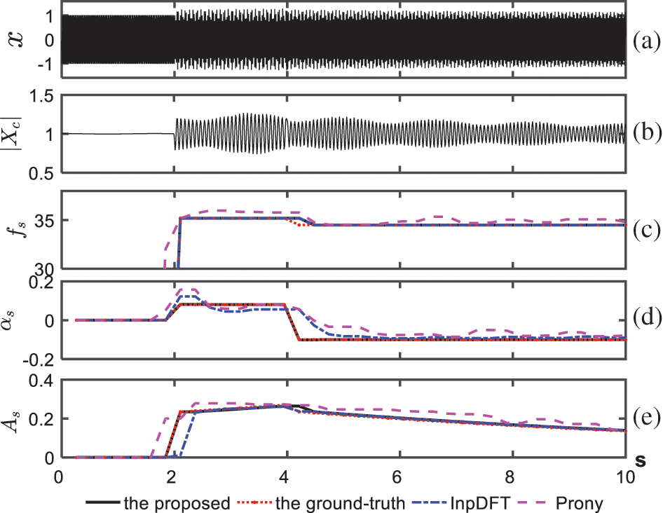
Figure 2: Synthetic SSR data and estimated results by using the proposed method and two other comparative methods for noise-free synthetic data, where each computational window applies N=50 synchrophasor data. (a) Instantaneous current x(t) (b) reported synchrophasor data |Xc|, (c) estimated fs, (d) estimated αs, and (e) estimated As

The proposed method applies a sliding window to identify the parameters of SSR, and each window contains N=50 synchrophasor data (i.e., 0.5 s data). The window is shifted N=2 each time, so N=2 synchrophasor data overlap between two successive windows. For the synchrophasors in Fig. 2b, the estimated fs, αs and As are shown as black curves in Figs. 2c–2e, while the true values are depicted as red dot curves. To compare the proposed method with the InpDFT method and Prony method, the same sliding window scheme and window data with N=50 were used in the three methods. Figs. 2c–2e also show the results obtained from the InpDFT and Prony methods, depicted as blue dot curves and magenta dot curves, respectively. As seen from the figure, the curves of the proposed method match better with the true values than those of the two comparative methods.

In another test, Gaussian noise was also added to the signal. According to our field data and those reported in the literature [24], the noises in practical PMU data are generally around a signal-to-noise ratio SNR = 45 dB. Thus, the paper considers noise with SNR = 40 dB. The results obtained from the proposed and two comparative methods are shown in Figs. 3b–3d. Since Prony is sensitive to noise, the results of Prony become worse, showing a large deviation from the ground truth under noisy conditions. The proposed method also coincides better with the true values than the InpDFT and Prony methods. Comparatively, the estimation of fs is more accurate than that of αs and As.

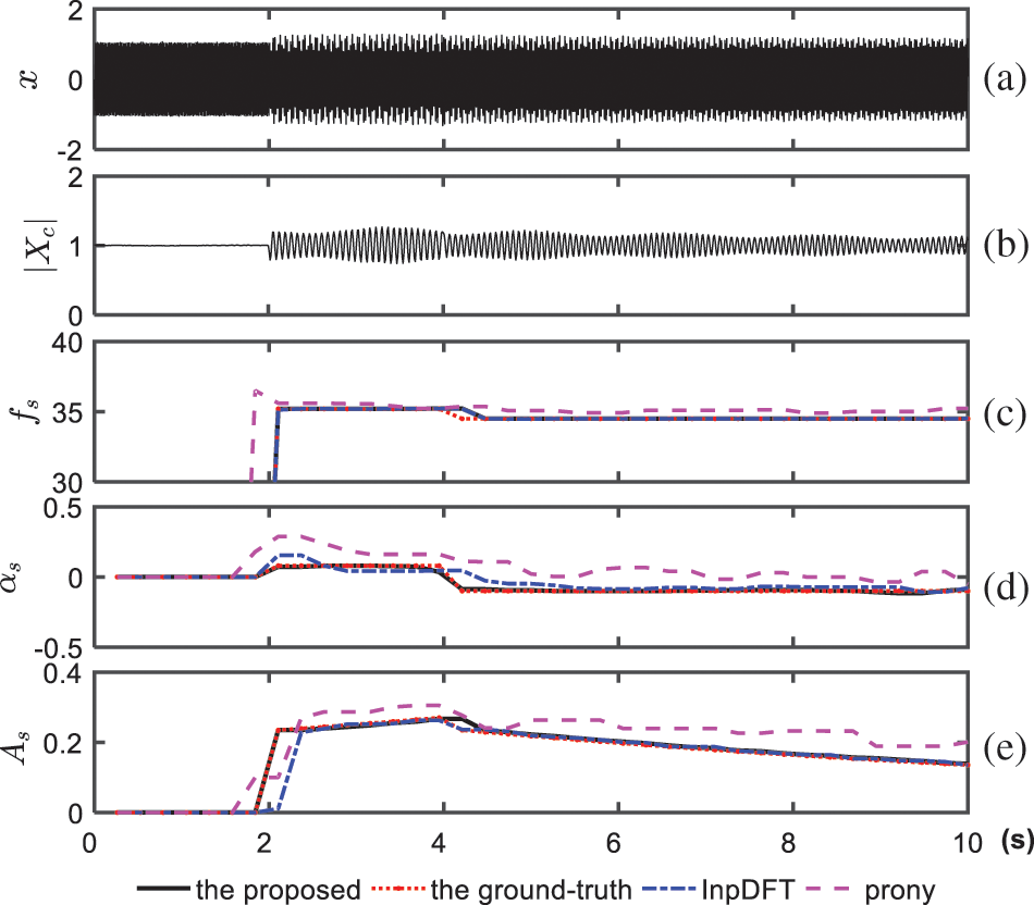
Figure 3: Synthetic SSR data and estimated results by using the proposed method and two other comparative methods for 40 dB noised synthetic data, where each computational window applies N=50 synchrophasor data. (a) Instantaneous current x(t) (b) reported synchrophasor data |Xc|, (c) estimated fs, (d) estimated αs, and (e) estimated As

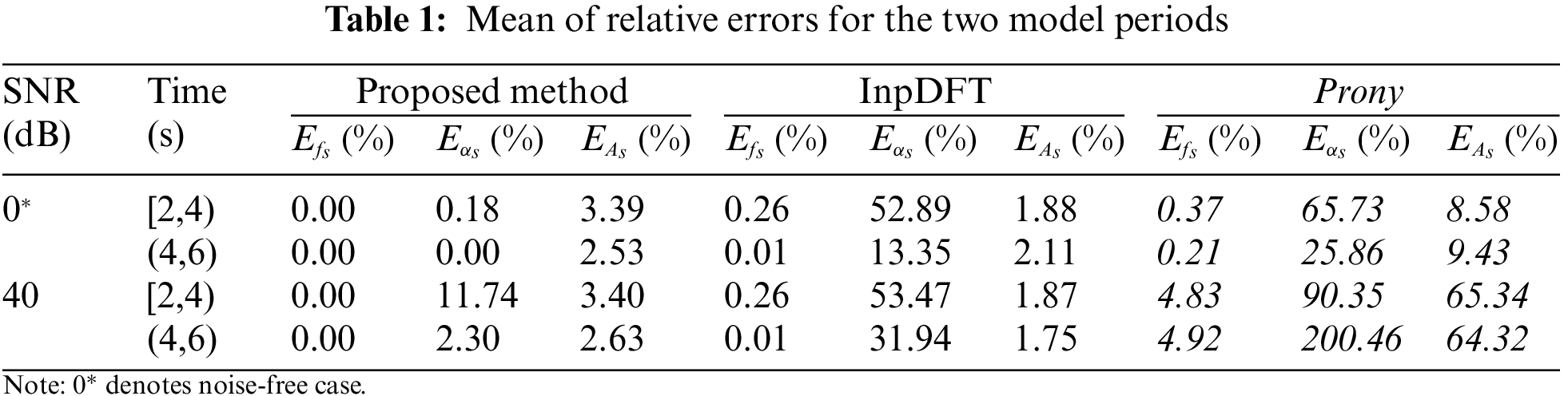
Furthermore, the mean errors of the three methods are displayed in Table 1 for two model periods, i.e., [2,4) s and (4,6] s, as shown in Fig. 2a. The mean errors Eb of each window were calculated as

Eb=mean(|b(t)−b~(t)|b(t)×100%)b:fs,αs,Ast∈[2,4)or(4,6](33)

where mean(⋅) is the mean operator and b(t) and b~(t) are the true and estimated parameter values at time t, respectively. In both noise-free and noisy conditions, the proposed method achieves a higher accuracy for fs and αs. It is clear that the estimation of αs from InpDFT is unacceptable. The reason is that [13] relies on DFT; thus, a longer window is required to overcome the spectral leakage issue due to the off-nominal f1. In the case that spectral leakage does not occur, InpDFT can achieve acceptable estimation of the three parameters by using short window data.

4.2 Simulated SSR

The proposed method was further tested by simulated SSR data. For this purpose, a series-compensated wind farm system was modeled in MATLAB/Simulink software, as shown in Fig. 4a. A sixth-order model of the induction machine is used, with a two-mass drive train model to represent the generator shaft. Figs. 4b and 4c show the control strategies of the grid-side converter (GSC) and the rotor-side converter (RSC), respectively. Table 2 provides the key system parameters, and further details of the simulation model can be found in [25].

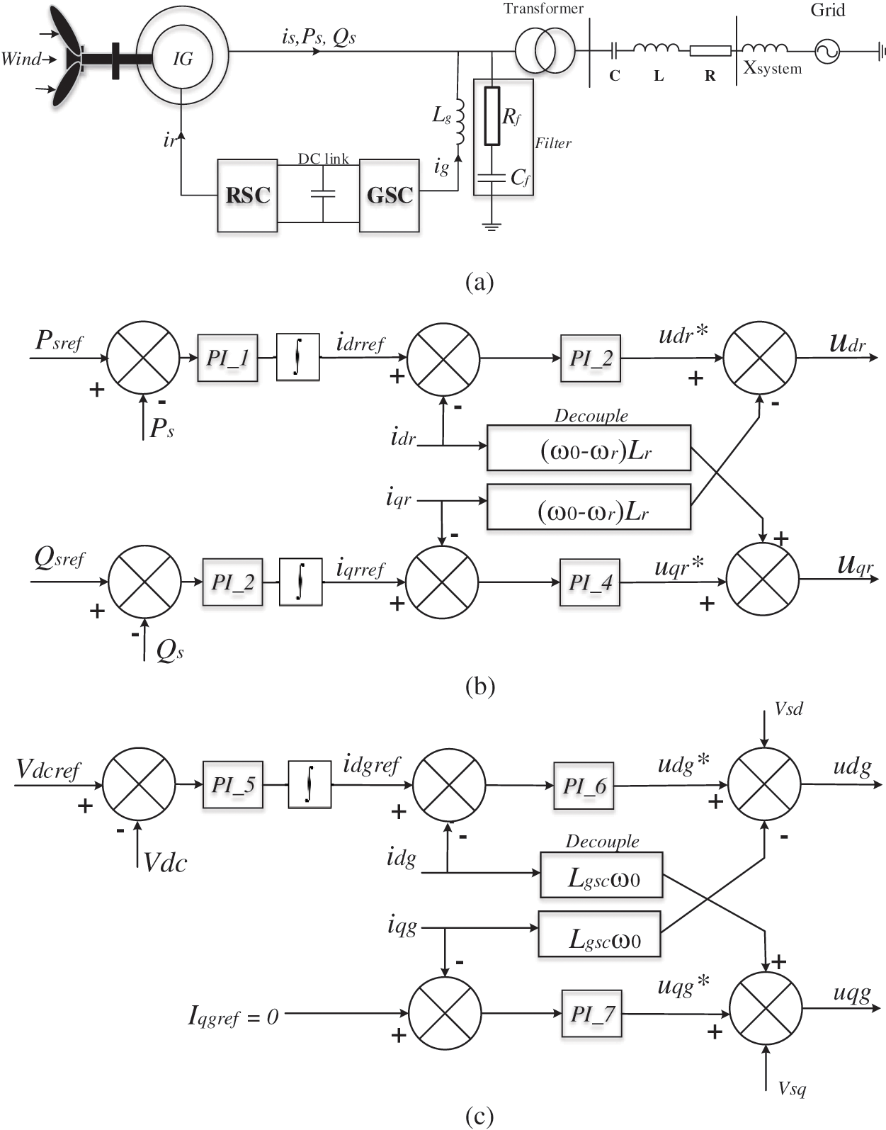
Figure 4: Simulated series-compensated DFIG-based wind farm. (a) System structure, (b) control block diagram of the RSC, and (c) control block diagram of the GSC

An SSR event is initiated at t=1 s when the series compensation level of the line is increased from 0.2 to 0.3. The wind speed is initially set as 8 m/s and gradually changes to 9 m/s. The waveform of the phase A current flowing through the line and the magnitude of the corresponding synchrophasors Xc are shown in Figs. 5a and 5b, respectively. Due to the change in wind speed, the SSR mode changes, which can be clearly observed from Fig. 5a.

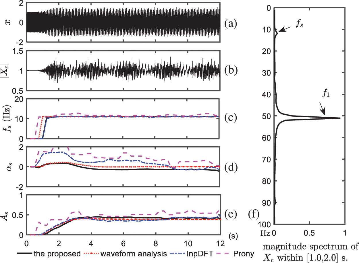
Figure 5: Simulated SSR data and results from the four methods. (a) Instantaneous current x(t) (b) reported synchrophasor data |Xc|, (c) estimated fs, (d) estimated αs, and (e) estimated As, and (f) the magnitude spectrum of Xc within [1,1.5] s

After the proposed method was performed on each window with N=50 synchrophasors, the estimated SSR parameters are shown as black lines in Figs. 5c–5e. Meanwhile, the results obtained from the InpDFT and Prony methods are also shown in Figs. 5c–5e. To evaluate the accuracy of the three methods, Figs. 5c–5e show the reference values obtained from the waveform-based analysis. For the waveform-based analysis, the frequency and amplitude were directly calculated from DFT with a long-length window, while the damping was computed by the amplitude difference of two successive data windows. From Figs. 5d and 5e, it can be seen that the damping and amplitude trends obtained from the proposed method are in good agreement with the waveform-based analysis. However, the Prony method provides an unsatisfactory estimation of damping and amplitude, and the InpDFT method exhibits a poor estimation of damping due to the spectral leakage of f1 shown in Fig. 5f.

4.3 Field Data

This subsection investigates the performance of the proposed method using practical SSR incidents that occurred in North China. Two sets of field data at different periods are used. Figs. 6a and 7a show the waveform data provided by the fault recorder with a sampling rate of 1000 Hz, while the magnitude of the corresponding synchrophasors is shown in Figs. 6b and 7b. It can be seen that the SSR mode varies over time. The possible reasons could be the tripping of wind generators and the change in the wind speed.

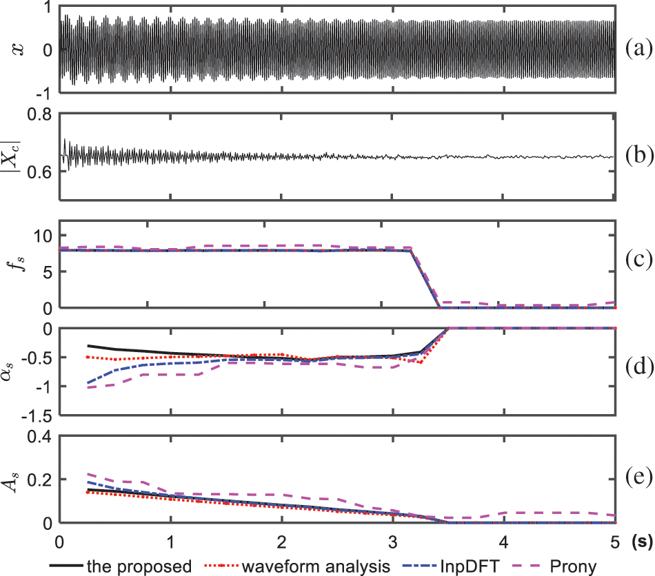
Figure 6: First set of field SSR data and estimated results from the four methods. (a) Instantaneous current x(t) (b) reported synchrophasor data |Xc|, (c) estimated fs, (d) estimated αs, and (e) estimated As

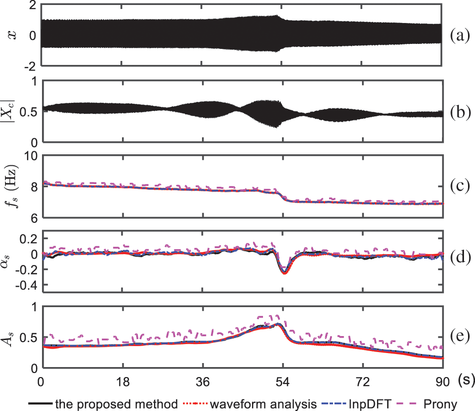
Figure 7: Second set of Field SSR data and estimated results from the four methods. (a) Instantaneous current x(t) (b) reported synchrophasor data |Xc|, (c) estimated fs, (d) estimated αs, and (e) estimated As

The estimation results of the first case are shown in Figs. 6c–6e. Similarly, the InpDFT and Prony methods are considered for comparison, and waveform-based analysis is used as a reference. According to the results, the estimation of the proposed method matches well with the reference value, while the damping results estimated by the two comparative methods deviate from those of the proposed method and waveform analysis.

The estimation results of the second case are shown in Figs. 7c–7e. Different from the first case, the off-nominal condition in the second period is not severe. As a result, the curves of the estimated parameters from the proposed and InpDFT methods match well, whereas the Prony method still cannot achieve satisfactory estimation and cannot effectively capture the variation in the damping and amplitude. The estimated fs varies between 7 and 8 Hz in Fig. 7c, which coincides with the results in [3], and the damping curves in Fig. 7d clearly show the rising and falling variation, which is consistent with the variation in the waveform amplitude. The two sets of experimental results demonstrate that the proposed method can capture the dynamic variation of the three parameters of the SSR component regardless of the spectral leakage effect.

5  Conclusion

This paper presented a Hankel-DMD-based method to identify SSR parameters using synchrophasor data. Through rigorous analytical derivation, it is revealed that SSRPI can be formulated as a DMD problem. By taking advantage of the Hankel matrix, which increases the modes of the subspace, the SSR parameters can be identified using a single channel of synchrophasor data within one second. Its performance has been verified using both simulation and field data. Comparative studies also demonstrate its superiority when compared with state-of-the-art algorithms. Therefore, it is expected that the proposed method can serve as an effective tool for wide area monitoring of SSR parameters.

Funding Statement: This work was supported by the China Key Technology Research on Risk Perception of Sub-Synchronous Oscillation of Grid with Large-Scale New Energy Access SGTYHT/21-JS-223.

Conflicts of Interest: The authors declare that they have no conflicts of interest to report regarding the present study.

Appendix A. Proof of the linear combination

Let H1(i) be the ith column of H1 in (13), given as

H1(i)=[Xc(i),Xc(i+1),…,Xc(i+L−1)]T(i=0,1,…,L−1)(34)

From (12), we obtain

H1(i)=QD(i)(35)

with

Q=[a1a2⋯ara1λ1a2λ2⋯arλra1λ12a2λ22⋯arλr2⋯⋯⋯⋯a1λ1L−1a2λ2L−1⋯arλrL−1]

and

D(i)=[λ1i,…,λri]T(36)

From (35), we can solve D(i) as follows:

D(i)=Q†H1(i)(37)

where Q† is the pseudo inverse of Q.

Let H2(i) be the ith column of H2 in (14), given as

H2(i)=[Xc(i+1),Xc(i+2),…,Xc(i+L)]T(i=0,1,…,L−1)(38)

Similar to (35), H2(i) is given by

H2(i)=QD(i+1)(39)

where i=0,1,…,L−1. Then, we have

D(i+1)=ΛD(i)(40)

with

Λ=diag(λj)(j=1,…,r)(41)

by using (36).

Thus, considering (37) and (40), we can rewrite (39) as

H2(i)=AH1(i)(42)

where a linear map A connects the ith column data of H1 and H2, given by

A=QΛQ†(43)

Finally, by extending the relation of the vector in (42) to the matrix, the connection of H2 and H1 is constructed as

H2=AH1(44)

where A is a linear map from H1 to H2.

References

1. Suriyaarachchi, D. H. R., Annakkage, U. D., Karawita, C., Jacobson, D. A. A. (2013). Procedure to study sub-synchronous interactions in wind integrated power systems. IEEE Transactions on Power Systems, 28(1), 377–384. DOI 10.1109/TPWRS.2012.2204283. [Google Scholar] [CrossRef]
2. Lawrence, C., Gross Jr, P. (2010). Sub-synchronous grid conditions: New event, new problem, and new solutions. Proceedings of the Western Protective Relay Conference, vol. 37, pp. 1–19. Spokane. [Google Scholar]
3. Xie, X., Xu, Z., Liu, H., Hui, L., Li, Y. et al. (2017). Characteristic analysis of subsynchronous resonance in practical wind farms connected to series-compensated transmissions. IEEE Transactions on Energy Conversion, 32(3), 1117–1126. DOI 10.1109/TEC.2017.2676024. [Google Scholar] [CrossRef]
4. Liang, W., Xie, X., Jiang, Q., Hui, L., Liu, H. (2015). Investigation of SSR in practical DFIG-based wind farms connected to a series-compensated power system. IEEE Transactions on Power Systems, 30(5), 2772–2779. DOI 10.1109/TPWRS.2014.2365197. [Google Scholar] [CrossRef]
5. Xie, X., Zhan, Y., Shair, J., Ka, Z., Chang, X. (2019). Identifying the source of subsynchronous control interaction via wide-area monitoring of sub/super-synchronous power flows. IEEE Transactions on Power Delivery, 35(5), 2177–2185. DOI 10.1109/TPWRD.2019.2963336. [Google Scholar] [CrossRef]
6. Li, P., Xiong, L., Wu, F., Ma, M., Wang, J. (2019). Sliding mode controller based on feedback linearization for damping of sub-synchronous control interaction in DFIG-based wind power plants. International Journal of Electrical Power & Energy Systems, 107(3), 239–250. DOI 10.1016/j.ijepes.2018.11.020. [Google Scholar] [CrossRef]
7. Li, P., Xiong, L., Wu, F., Ma, M., Huang, S. et al. (2022). Energy-shaping L2-gain controller for PMSG wind turbine to mitigate subsynchronous interaction. International Journal of Electrical Power & Energy Systems, 135(3), 107571. DOI 10.1016/j.ijepes.2021.107571. [Google Scholar] [CrossRef]
8. Alawasa, K. M., Mohamed, Y. A. I. (2015). A simple approach to damp SSR in series-compensated systems via reshaping the output admittance of a nearby VSC-based system. IEEE Transactions on Industrial Electronics, 62(5), 2673–2682. DOI 10.1109/TIE.2014.2363622. [Google Scholar] [CrossRef]
9. Netto, M., Mili, L. (2017). A robust prony method for power system electromechanical modes identification. Proceedings of the IEEE PES General Meeting, 18, 167–173. DOI 10.1109/PESGM.2017.8274323. [Google Scholar] [CrossRef]
10. Ning, Z., Trudnowski, D. J., Pierre, J. W., Mittelstadt, W. A. (2008). Electromechanical mode online estimation using regularized robust RLS methods. IEEE Transactions on Power Systems, 23(4), 1670–1680. DOI 10.1109/TPWRS.2008.2002173. [Google Scholar] [CrossRef]
11. Laila, D. S., Messina, A. R., Pal, B. C. (2009). A refined Hilbert-Huang transform with applications to inter-area oscillation monitoring. IEEE Transactions on Power Systems, 24(2), 610–620. DOI 10.1109/TPWRS.2009.2016478. [Google Scholar] [CrossRef]
12. Arrieta Paternina M. R., Tripathy R. K., Zamora-Mendez A., Dotta D. (2019). Identification of electromechanical oscillatory modes based on variational mode decomposition. Electric Power Systems Research, 167(3), 71–85. DOI 10.1016/j.epsr.2018.10.014. [Google Scholar] [CrossRef]
13. Yang, X., Zhang, J., Xie, X., Xiao, X., Wang, Y. (2020). Interpolated DFT-based identification of sub-synchronous oscillation parameters using synchrophasor data. IEEE Transaction on Smart Grid, 11(3), 2662–2675. DOI 10.1109/TSG.2019.2959811. [Google Scholar] [CrossRef]
14. Ree, J. D. L., Centeno, V., Thorp, J. S., Phadke, A. G. (2010). Synchronized phasor measurement applications in power systems. IEEE Transactions on Smart Grid, 1(1), 20–27. DOI 10.1109/TSG.2010.2044815. [Google Scholar] [CrossRef]
15. Vanfretti, L., Baudette, M., Al-Khatib, I., Almas, M. S., Gjerde, J. O. (2013). Testing and validation of a fast real-time oscillation detection PMU-based application for wind-farm monitoring. Proceedings of the First International Black Sea Conference on Communications & Networking, pp. 216–221. Batumi. [Google Scholar]
16. Wang, Y., Jiang, X., Xie, X., Yang, X., Xiao, X. (2021). Identifying sources of subsynchronous resonance using wide-area phasor measurements. IEEE Transactions on Power Delivery, 36(5), 3242–3254. DOI 10.1109/TPWRD.2020.3037289. [Google Scholar] [CrossRef]
17. Zhang, F., Cheng, L., Gao, W., Huang, R. (2019). Synchrophasors-based identification for subsynchronous oscillations in power systems. IEEE Transactions on Smart Grid, 10(2), 2224–2233. DOI 10.1109/TSG.2018.2792005. [Google Scholar] [CrossRef]
18. Schmid, P. J., Sesterhenn, J. (2008). Dynamic mode decomposition of numerical and experimental data. Journal of Fluid Mechanics, 656, 5–28. DOI 10.1017/S0022112010001217. [Google Scholar] [CrossRef]
19. Solaija, M. S. J., Saleem, S., Khurshid, K., Hassan, S. A., Kamboh, A. M. (2018). Dynamic mode decomposition based epileptic seizure detection from scalp EEG. IEEE Access, 6, 38683–38692. DOI 10.1109/ACCESS.2018.2853125. [Google Scholar] [CrossRef]
20. Barocio, E., Pal, B. C., Thornhill, N. F., Messina, A. R. (2014). A dynamic mode decomposition framework for global power system oscillation analysis. IEEE Transactions on Power Systems, 30(6), 2902–2912. DOI 10.1109/TPWRS.2014.2368078. [Google Scholar] [CrossRef]
21. Gao, B., Wang, Y., Xu, W., Yang, G. (2020). Identifying and ranking sources of SSR based on the concept of subsynchronous power. IEEE Transactions on Power Delivery, 35(1), 258–268. DOI 10.1109/TPWRD.2019.2916848. [Google Scholar] [CrossRef]
22. Tu, J. H., Rowley, C. W., Luchtenburg, D. M., Brunton, S. L., Kutz, J. N. (2014). On dynamic mode decomposition: Theory and applications. Journal of Computational Dynamics, 1, 291–320. [Google Scholar]
23. Filho, E. V., dos Santos, P. L. (2019). A dynamic mode decomposition approach with hankel blocks to forecast multi-channel temporal series. IEEE Control Systems Letters, 3(3), 739–744. DOI 10.1109/LCSYS.2019.2917811. [Google Scholar] [CrossRef]
24. Brown, M., Biswal, M., Brahma, S., Ranade, S. J., Cao, H. (2016). Characterizing and quantifying noise in PMU data. Proceedings of the Power & Energy Society General Meeting, pp. 1–5. Boston. [Google Scholar]
25. Gao, B., Torquato, R., Xu, W., Freitas, W. (2019). Waveform-based method for fast and accurate identification of subsynchronous resonance events. IEEE Transactions on Power Systems, 34(5), 3626–3636. DOI 10.1109/TPWRS.2019.2904914. [Google Scholar] [CrossRef]