Studies on Performance of Distributed Vertical Axis Wind Turbine under Building Turbulence

1  Introduction

The world’s mainstream wind turbines are currently large and medium-sized horizontal axis wind turbines with mature technology and uniform standards; research on vertical axis wind turbines is relatively lagging behind, mainly in the stage of wind tunnel experiments and field tests, with small and medium-sized turbines. A horizontal axis wind turbine has the benefits of a high operating wind speed, stable aerodynamic load, and relatively simple aerodynamics, but it also has the disadvantages of a yaw wind device and high noise, making it unsuitable for use in urban areas with low wind speeds and high turbulence intensity [1,2]. However, even in the presence of strong turbulence, the vertical axis wind turbine can achieve a significant power coefficient and has the features of all wind directions [3,4]. At the same time, the vertical axis wind turbine has a basic structure and few parts, making it easy to install and maintain; the blade is often of constant cross-section design, and manufacturing costs are minimal. In addition, the vertical axis wind turbine offers reduced operation noise, a beautiful appearance, and takes up less area, better structural scalability, and higher system stability [5]. The installation in the city can enhance the beauty of the city. As a result, vertical axis wind turbines are common in distributed generating. However, due to the limitations of the installation site, the upstream building disturbance may have an impact on the downstream space in terms of wind speed, direction, and turbulence intensity, and the aerodynamic performance of downstream wind turbines may be influenced further when these parameters are changed. Therefore, it is necessary to clarify how the building turbulence impacts the performance of downstream wind turbines.

Early international scientists used a two-dimensional flow field to simulate and determine the aerodynamic performance of vertical axis wind turbines, and the applicability of sliding mesh in the computation of vertical axis wind turbine blade technology was validated [6–8]. In 1998, the British scientist Dr. Derek Taylor [9] first proposed building a roof wind energy system, with the roof designed to improve the function of wind power and wind turbines installed on the roof. In 2009, Hong Kong Scholars Lu et al. [10] used the CFD numerical analysis approach to investigate the feasibility of wind energy utilization in high-rise buildings and to improve wind energy utilization. Wind energy use can be improved by increasing wind speed and modifying building structures. In 2010, Salame’s team [11] at the IEEE PES general conference summarized the forms and characteristics of building-wind-turbine combinations from around the world, demonstrating the enormous potential of wind turbines in urban settings. Xu et al. [12] simulated the roof structure layout and surrounding buildings using the CFD method on the outer wall face of a science and technology museum, as well as the roof structure layout and adjacent buildings, under various wind directions and wind speeds. The calculations show that under various wind directions and speeds, the layout of buildings and buildings will generate differing degrees of airflow interference.

Turbulence intensity can increase mechanical stress on turbine components and reduce turbine life. For small wind turbines, obstacles such as buildings and trees may cause high levels of free flow turbulence [13–15]. Abohela et al. [16,17] used CFD techniques to model and examine the wind around buildings and the rationale that affects the location of wind turbines. Scholars in the United States have investigated the performance of H-type and S-type vertical axis fans in terms of wind speed and turbulence, as well as roof pitches under various wind directions, to modify the wind downstream and manage the operating efficiency of downwind wind turbines [18–22]. The research object in this work is a combined vertical axis wind turbine with Φ-type outer blades as lift blades and S-type inner blades as resistance blades. By varying the wind speed and replicating the working conditions under both wall-existing and wallless settings, the impact of wall turbulence by a disturbance on the performance of vertical axis wind turbine generators is investigated.

2  Generator Installation and Specific Parameters

Turbulence formed as the incoming wind comes in from the wall and passes over the wind turbine due to the presence of the wall, and the presence of turbulence will have a substantial impact on the wind turbine’s performance. As a result, more research into the turbulence distribution induced by the flow field through the building is needed.

The research object in this work is a 700 W mixed vertical axis wind turbine. The wind turbine is located in the Jinchuan Development Zone, Hohhot, Inner Mongolia Autonomous Region’s experimental base, which is situated in an open area with sufficient wind resources throughout the year, as shown in Fig. 1.

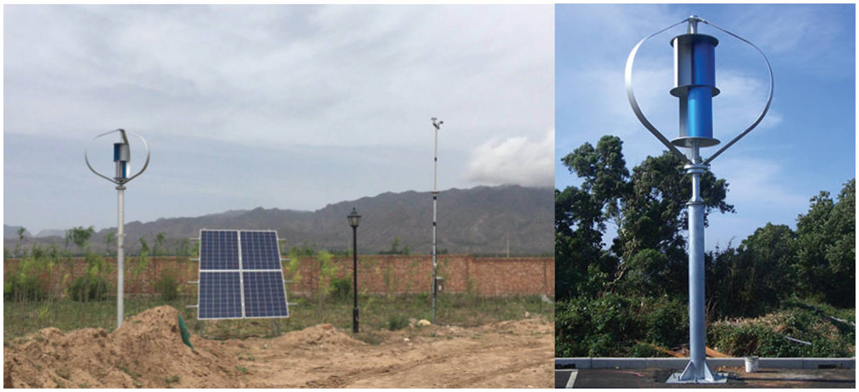
Figure 1: Example of decentralized wind power generation (test site live shooting)

This study focuses solely on the wind turbine’s wind wheel. The characteristics affecting the wind turbine and the wall are depicted in Table 1.

3  Numerical Simulation Method

3.1 Geometric Modeling

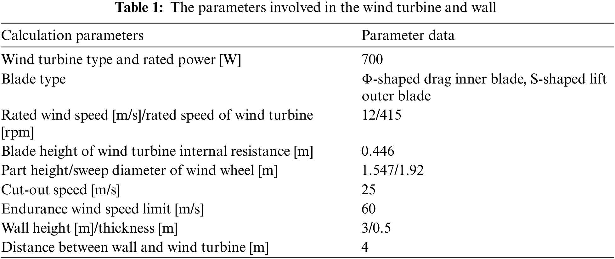
The 700 W vertical axis wind turbine is simulated and modeled in this work. The vertical axis wind turbine is simplified since some components have little impact on aerodynamics. The diameter of the wind turbine’s internal resistance blade is 0.357 m, the height of the internal resistance vanes is 0.446 m, the height of the wind turbine is 1.547 m, and the sweeping diameter of the wind turbine is 1.92 m after simplification. The dimensions of the model are displayed in Fig. 2.

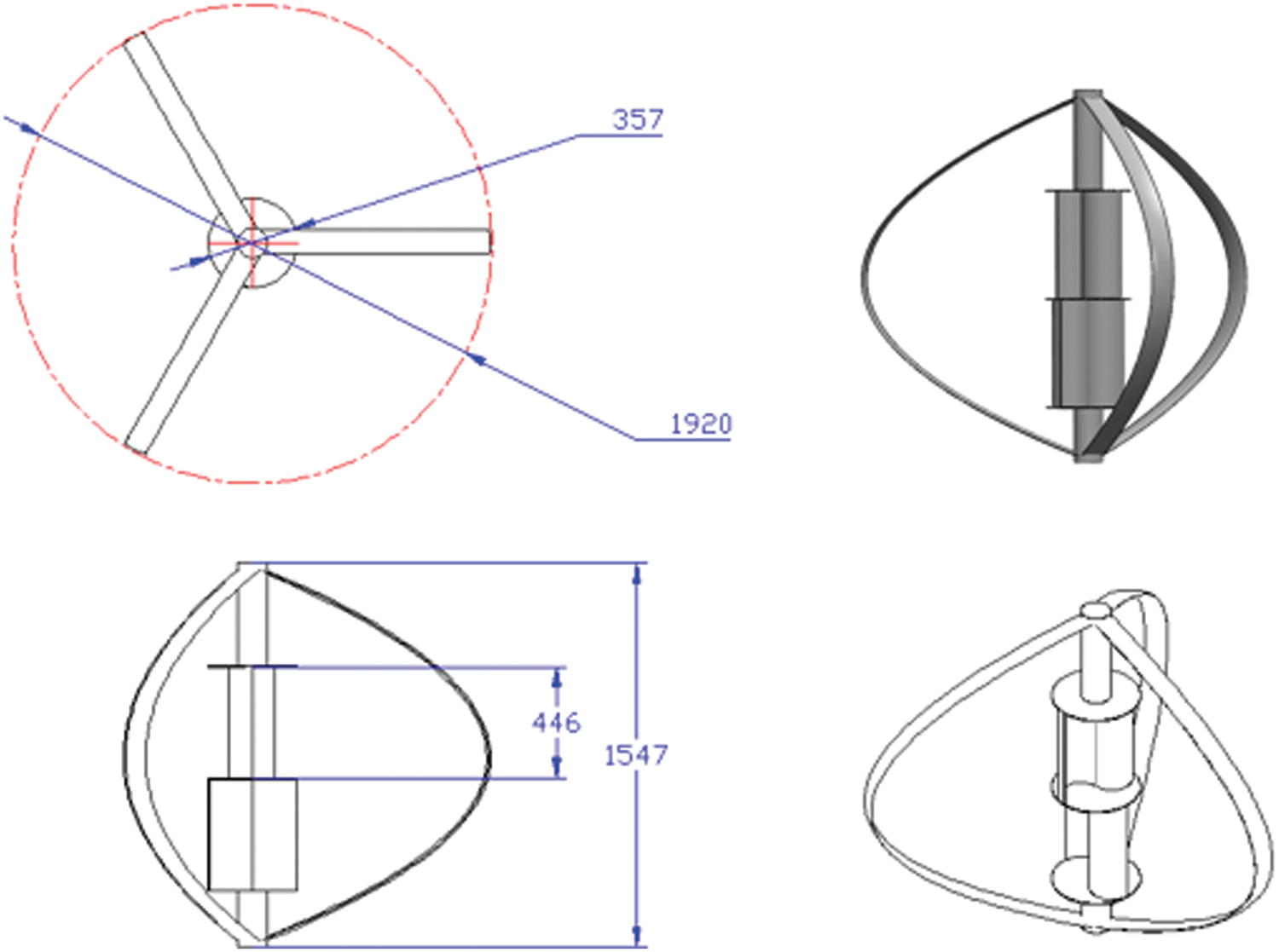
Figure 2: Modeling sketch of horizontal axis wind turbine

The relative height between the upper edge of the wall and the wind turbine’s wind wheel is ∆ H = 0 m, the horizontal relative distance is 4 m, and the thickness is 0.5 m to establish a general trend of the wall’s impact on the wind turbine’s performance. The oncoming wind blew past the wind turbine and over the wall. The incoming wind direction is depicted, as well as the placement diagram of the wall and wind turbine generator in Fig. 3.

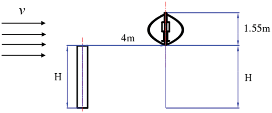
Figure 3: Drawing of wind turbine position

3.2 Calculation Domain Creation and Meshing

3.2.1 Calculation Domain Creation

In the computation domain, the method of managing blockage rate Q is used. The calculation domain for this paper is 20D×6D×6D (D denotes the sweeping diameter of wind turbines). According to the dimensions of the wind turbine indicated above, the blockage rate is between 2.5% and 7%, which fits the criteria throughout the entire calculation region [23,24]. The size of the calculation domain is shown in Fig. 4.

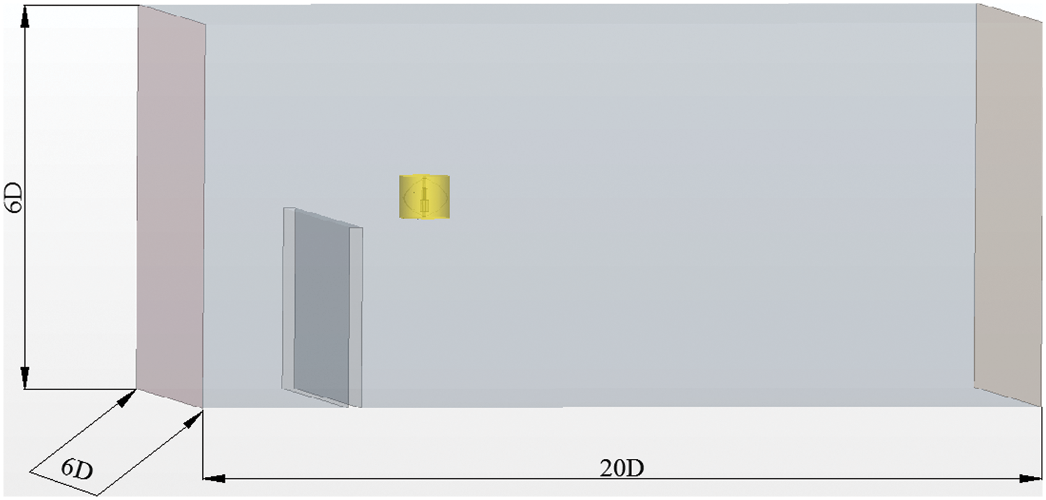
Figure 4: Computational domain size

3.2.2 Meshing

In this paper, the hexahedral unstructured grid is chosen for a grid division. The wind turbine and its wake area, as well as the wind turbine rotation area and wake area, are subjected to grid densification to better monitor wind speed and turbulence variations surrounding the wall, as shown in Figs. 5 and 6.

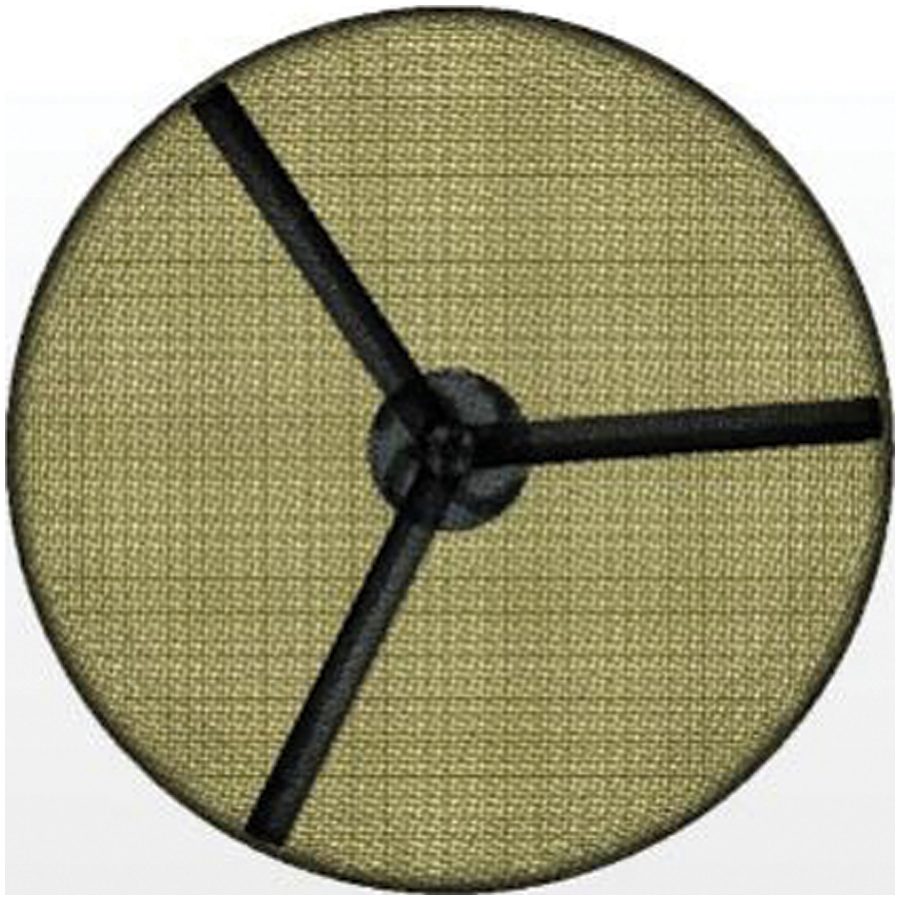
Figure 5: Wind turbine and rotating domain

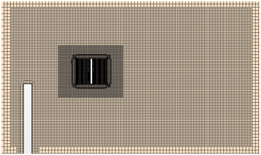
Figure 6: Mesh around the wall and rotating domain

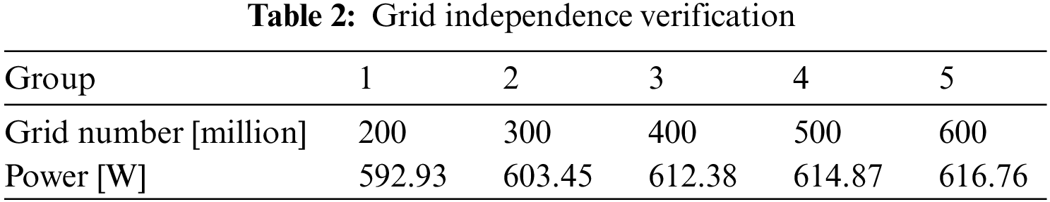
For meshing, a three-layer hexahedral mesh boundary is chosen, and a set of five meshes that converge satisfactorily under rated conditions is collected to validate their independence from one another. According to the calculations shown in Table 2, the power change rate between Groups 1 and 3 is greater than 1.45%, implying that grid numbers ranging from 2 million to 4 million can have a significant impact on the outcomes. Groups 3 to 5 disclose no more than 0.4% of the change rate when the grid number exceeds 4 million, implying that the grid number plays a minor influence in this range. As a result, in future numerical calculations, a grid number of 4 million is used to save computational time and resources.

Wind turbine power is an important metric for determining a wind turbine’s functioning capability.

P=T×n/9550(1)

T——Wind turbine impeller torque, Nm;

n——Wind turbine blade speed, rpm.

Table 2 is derived using the formula for calculating wind turbine power (1). Calculating the wind turbine’s speed allows us to determine the time required to rotate n degrees or the time step:

t=nπ180ω(2)

3.3 Setting of the Physical Model and Boundary Conditions

3.3.1 Setting of a Physical Model

In comparison to the standard model, the realizable model uses unique mathematical approaches to confine normal stress and includes a turbulent viscous formula [25] to handle the problem of negative-positive stress due to a large time-averaged strain rate. The turbulent dissipation rate has a new transfer equation added to it so that it can better depict energy transfer in general space. The transport equations of k and ε are:

∂(ρk)∂t+∂(ρkuj¯)∂xj=∂∂xj[(μ+μtσk)∂k∂xj]+Pk+Gb−ρε−YM+Sk(3)

∂(ρε)∂t+∂(ρεuj¯)∂xj=∂∂xj[(μ+μtσε)∂ε∂xj]+ρC1S¯ε−C2ρε2k+vε+Cε1εkCε3Gb(4)

In the formula:

μt=Cμρk2ε,Cμ=1A0+ASU∗kε

C1=max{0.43,ηη+5},η=kεS¯

S¯=2Sij¯Sij¯,Sij¯=12(∂ui¯∂xj+∂uj¯∂xi)

As=6cos⁡ϕ,ϕ=13cos−1⁡(6W)

W=Sij¯Sjk¯Ski¯Sij¯Sij¯,U∗=Sij¯Sij¯+Ωij¯Ωij¯¯

Ωij¯¯=Ωij−2εijkωk,Ωij=Ωij¯−εijkωk

Among them, A0 = 4.04, σk = 1.0, σε = 1.2, Cε1=1.44,C2=1.9; When the main direction is parallel to the direction of gravity, Cε3=1.0. When the shear flow is perpendicular to the gravitational direction in the mainstream direction, Cε3=0. Ωij¯ is a time-averaged rotational velocity tensor observed in a reference system with angular velocity ωk. For the irrotational flow field, the second item in the root of the formula U∗ is zero, which is used to characterize the effect of rotation.

A realizable model is more accurate in predicting rotational flow, strong adverse pressure gradient boundary layer flow, separated flow, and secondary flow. The treatment of strong bending streamlines, vortices, and rotating flows is superior to other models. The disadvantage of this method is that the effect of average rotation is taken into account when defining turbulent viscosity, so the natural turbulent viscosity cannot be provided when calculating the rotational and static flow regions [26]. This model can ensure good accuracy and be better applied to bending, rotating, and rotating streamlines [27].

3.3.2 Boundary Conditions

Three-dimensional models, hidden transient solutions, separation solvers, gas, and equations are among the options available. In the Realizable turbulence model, the rotation rate is set to n = 415 rpm, and the vertical axis wind turbine is numerically simulated at five different wind speeds (v1 = 6 m/s, v2 = 9 m/s, v3 = 12 m/s, v4=15 m/s, v5 = 18 m/s). With a relative pressure of 0 Pa, the computation domain consists of wind speed as the entrance and pressure as the outlet.

3.4 Time Step Setting for Calculating Model Parameters

Calculating the wind turbine’s speed allows us to determine the time required to rotate n degrees or the time step:

t=nπ180ω(5)

The maximum physical time in this article is 5 s, the time step is 0.001 s, and the internal iteration is 5.

4  Analysis and Verification of Simulation

4.1 Numerical Simulation Results under Wallless Turbulence

The basic mechanics of a wind turbine is simulated at different incoming wind speeds ( v1 = 6 m/s, v2 = 9 m/s, v3 = 12 m/s, v4=15 m/s, v5 = 18 m/s) to understand the performance of the wind turbine and test the accuracy of numerical calculations. The calculation results of incoming wind speeds of 12 and 15 m/s are selected for comparison to facilitate observation and analysis. This paper will use the ratio of the distance L from the wind turbine in the horizontal direction to the wind turbine radius R to draw the curve and the curve of the change of speed ratio to assess the wake of a vertical axis wind turbine under different wind speeds (the ratio of maximum speed to incoming wind speed is VL/V0).

The horizontal speed variation trend under different incoming wind speeds is generally the same, as shown by the variation curve of wind speed variation in Fig. 7a, and the speed at −2R has a decreasing trend. The wind speed at the position of the wind turbine generator −1R~1R will change considerably, and the wind speed at position 0 of the wind turbine will reach its maximum. The wind speed ratio at the wind turbine position reaches its maximum, and the maximum wind speed ratio can reach 1.4 when the incoming wind speed is 18 m/s, indicating that the wind energy utilization rate at the wind turbine position reaches its maximum, according to the change curve of the wind speed ratio in Fig. 7b. The wind speed ratio is the lowest at 1R at the trailing edge of the wind turbine, and it is only 0.2 when the incoming wind speed is 6 m/s, which is when the wind energy loss is the greatest. This is because when the wind passes through the fan, the fan’s rotation causes a substantial disturbance in the wind speed at the fan’s wake area, and the disturbance effect at 1R at the trailing edge of the wind turbine wheel has reached its maximum. When the entering wind speed is 6, 9, or 12 m/s, the wind speed ratio in the fan’s wake area tends to 1 at 5R, and when the incoming wind speed is 15 and 18 m/s, it tends to 1 at 7R and 8R, respectively. This demonstrates that the wind speed variation trend in the vertical axis fan’s wake region is consistent under various incoming wind speeds and eventually approaches the incoming wind speed, the length of the wake will vary depending on the speed of the approaching wind and the greater the wind speed is the greater the wake’s influence ranges.

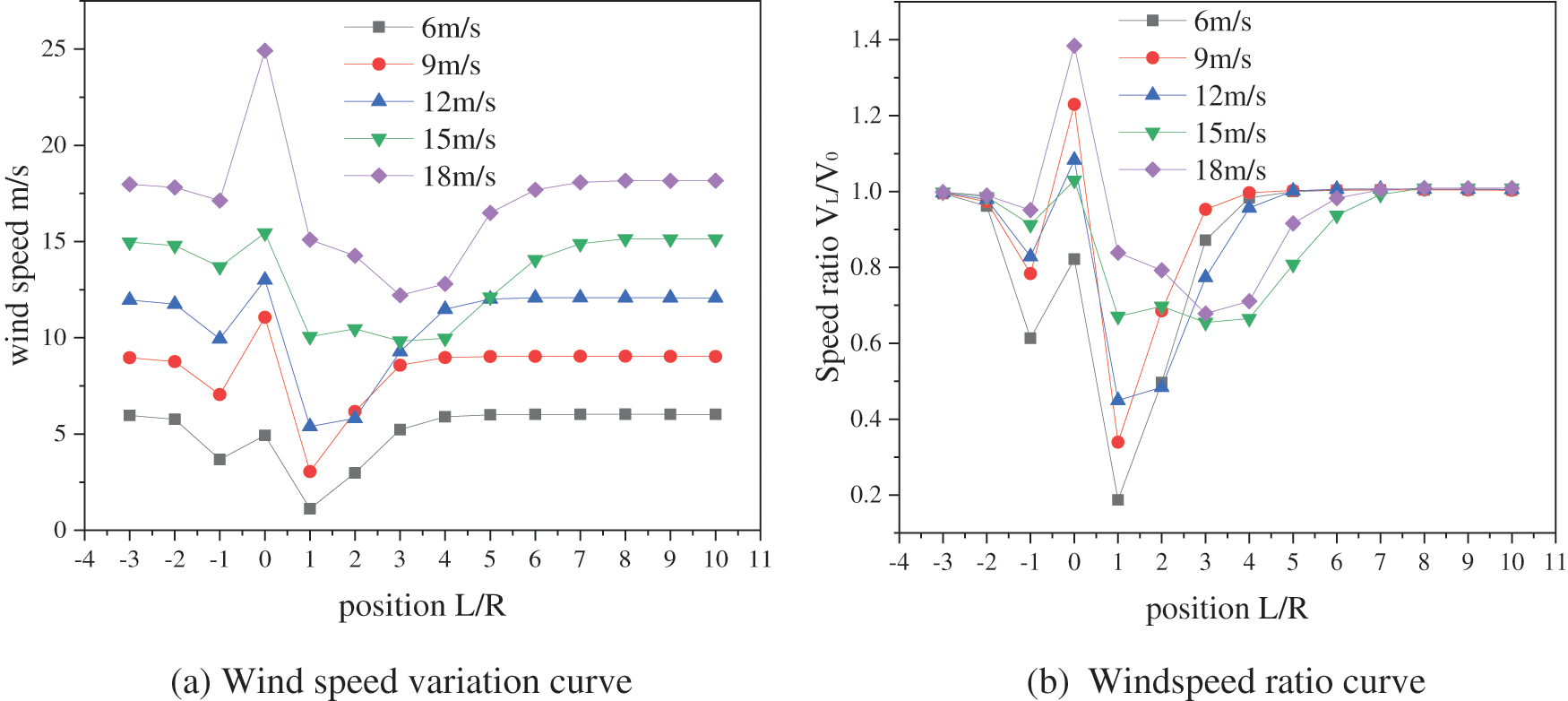
Figure 7: Curve of horizontal wind velocity variation with inlet wind velocity

The power using coefficient reaches the decide value when the turbine speed and the wind speed achieve the optimal ratio, according to the Betz theory. Therefore, when the optimal tip speed ratio of the wind turbine is 3.48, as can be observed in Fig. 8a, the power increases as the incoming wind speed increases. The power increasing rate tends to be flat when the incoming wind speed reaches 15 m/s. The wind pressure on the wind turbine blade surface increases as the wind speed increases, increasing the lift on the outer blade and the thrust on the internal resistance vanes, resulting in increased blade torque and output power. Furthermore, the numerical simulation power curve’s growing condition is compatible with the power curve provided by the Wind turbine manufacturer, and the error is within the permissible range, confirming the simulation’s accuracy.

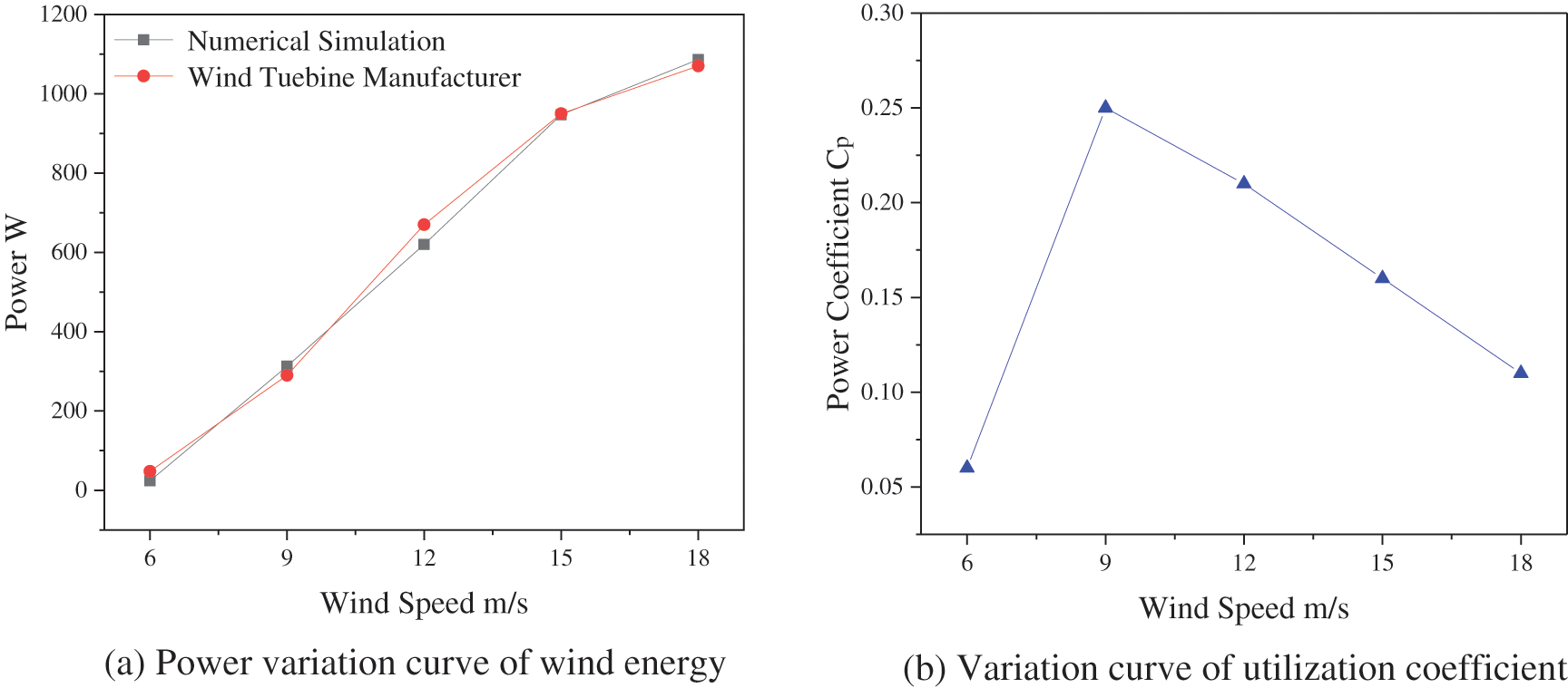
Figure 8: Variation curve of power and power coefficient with incoming wind speed without wall disturbance

The variation curve of the wind energy utilization coefficient, as shown in Fig. 8b, shows that the wind energy utilization coefficient shows a changing growth trend when the incoming wind speed is 6, 9 m/s and that the wind energy utilization coefficient decreases with increasing wind speed after 9 m/s. This is because the fan’s power is only 23.9 W when the incoming wind speed is 6 m/s, and the wind energy utilization coefficient improves greatly when the wind speed is 6~9 m/s; when the wind speed surpasses 9 m/s, the blade’s rotation speed remains unchanged. The larger the loss of wind energy traveling through the blade and the lower the wind energy utilization coefficient, the higher the wind speed.

4.2 Numerical Simulation and Results under Wall-Existing Turbulence

Fig. 9 shows that as the incoming air travels through the wall, there is a region of swirling turbulence in the upper and lower regions of the fan, and the wall-generated tangential wind velocity has a major impact on the wind turbine performance. The monitoring stations are placed within a specified ratio area, including the ratio of a certain horizontal distance to the wind turbine radius, to examine the effect range of the turbulent region on the wind turbine (L/R = −6,…, 14, scale 1) and the ratio of the vertical distance to the wind turbine height (H/h = −3,…, 3, scale 0.5). The velocity ratio (the ratio of the maximum speed to the incoming wind speed, v/v0) and the change curve of the velocity ratio (the ratio of the maximum speed to the incoming wind speed, v/v0) are displayed alongside the average maximum wind speed at the monitoring point.

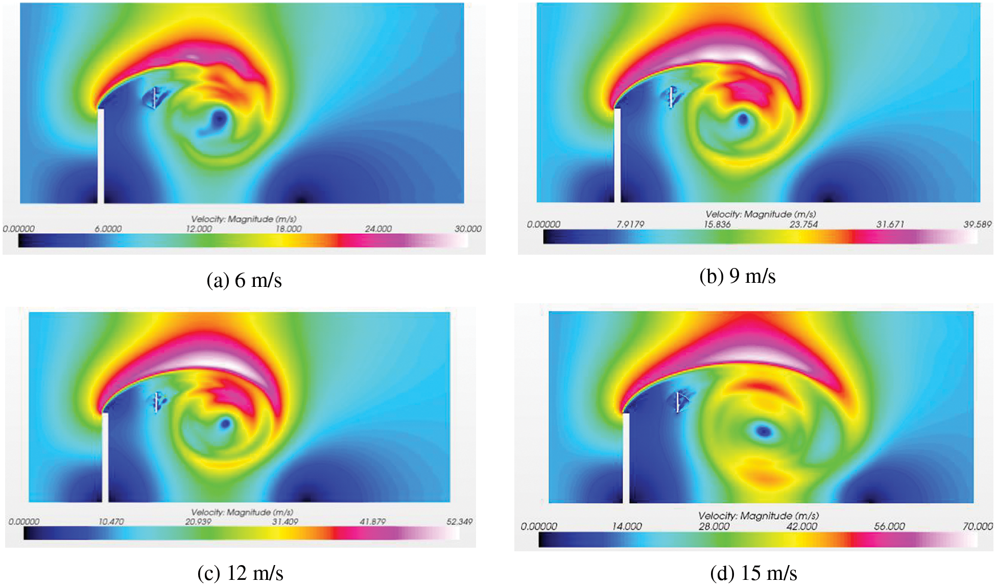
Figure 9: Wind turbine speed distribution diagram under wall-existing conditions

Fig.10 implies that for both walled and wallless settings, the tendency of how wind speed varies with incoming wind speed is the same. However, because there is a 4 m wall in front of the fan, the wind is turbulent on the horizontal axis in the upstream and downstream sections of the fan—the higher the entering wind speed is, the larger the wind speed changes. In the 2R~13R interval, the wind speed reaches the wind turbine cutoff, which is 25 m/s, and the wind turbine ceases to generate power. The wind speed in the range of 6R~10R exceeds the wind speed limit (60 m/s) after reaching 18 m/s; therefore, the wind turbine structure will be destroyed in this range. The area where wall turbulence can damage the wind turbine downstream is also approximately 14R when the wind speed ratio at the 14R position approaches 1. The wind speed is plotted against the incoming wind speed in graphs (c) and (d). The bottom edge of the wind turbine (at approximately 0.5 H of height) will disrupt the wind speed here to some extent due to wind turbine rotation. The wind speed ratio is reasonably stable and close to 1 in the height range of 0–1 H, indicating that the extent of the wall disruption is less influenced. The position at 1.5H is the most influenced by wall interference. In conclusion, the wind turbine should be installed as far away from the turbulence area or low disturbance area as practicable.

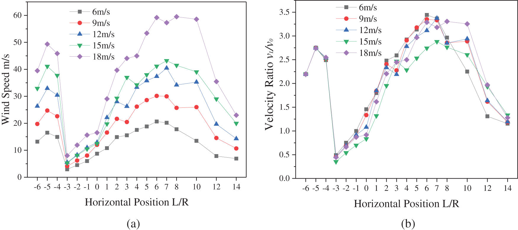
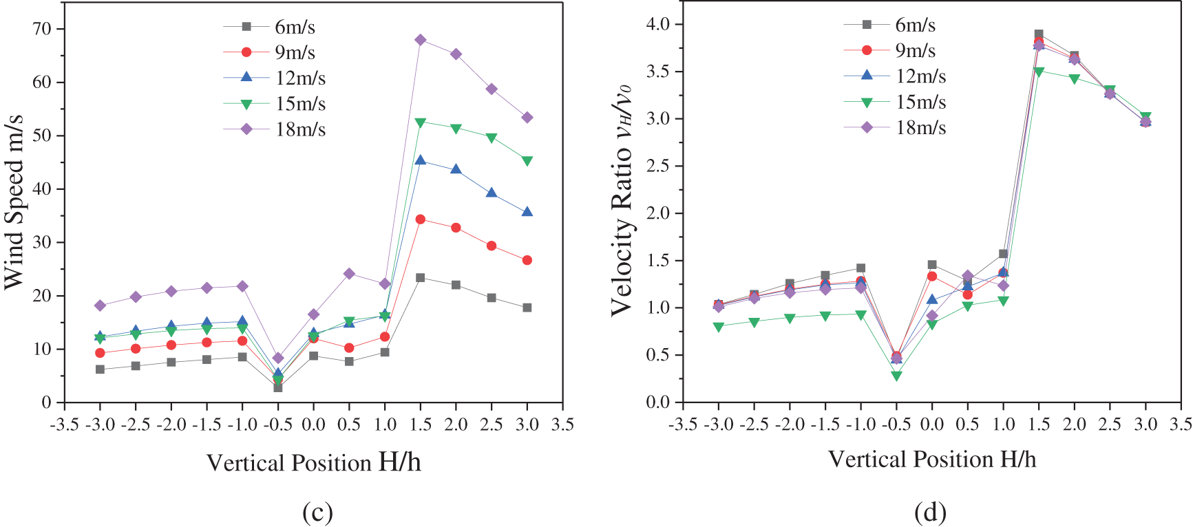
Figure 10: Variation curves of wind speed with incoming wind speed under wall-existing conditions

4.3 Comparison and Analysis of Simulation Results with Wall-Existing and Wallless Turbulence

The average wind speed is observed at the upper edge, lower edge, center, and windward blade of a wind turbine under two distinct scenarios to study the influence of building turbulence on wind speed at a wind turbine. The wind speed ratio (the ratio of wind speed under wall-existing conditions to that under the wallless condition, vw/v0) is computed and plotted against the flow wind speed curve.

Fig. 11 shows that when the incoming wind speed is below 12 m/s, the wind speed at the wind turbine position is higher than when the incoming wind speed is below 12 m/s, and when the incoming wind speed is above 12 m/s, the wind speeds at both the wind turbine center and blade position are lower than when the incoming wind speed is above 12 m/s. The bottom edge of the wind turbine is most affected by the whirling turbulence of the wall, while the higher edge is least affected. This phenomenon can be illustrated using the velocity distribution map of the wall in Fig. 6. The vortex turbulent zone of the wall is not separated from the fan’s bottom edge and the leeward blade location at wind speeds below 12 m/s. The wind speed in the turbulent part of the vortex is higher than the entering value, and some turbulent regions will increase the wind speed at the wind turbine location.

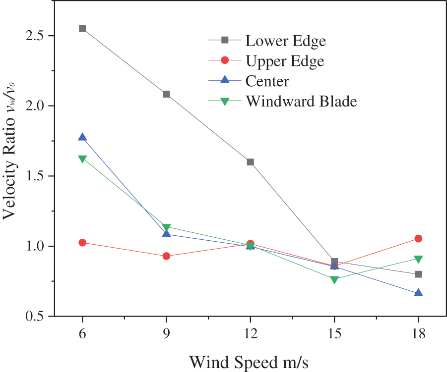
Figure 11: Variation curves of the wind turbine position velocity ratio with incoming wind speed

The power variation and the wind energy utilization coefficient under the two operating conditions are plotted based on the calculation results, as shown in Fig. 12.

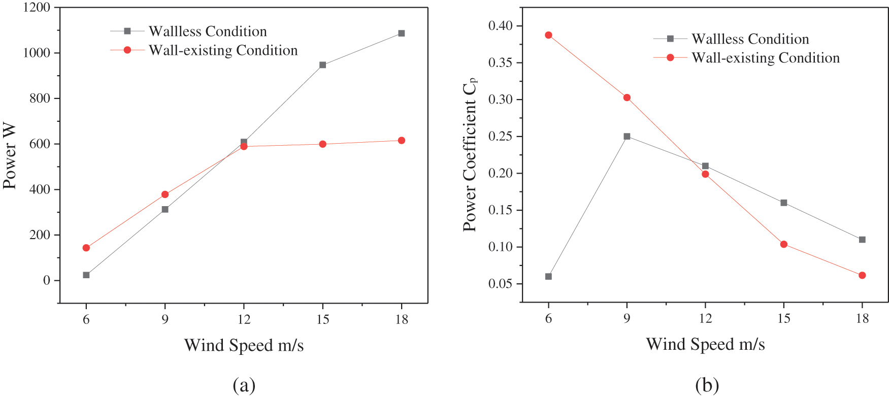
Figure 12: Variation curves of power and power coefficient

In both cases, the power and wind energy utilization coefficient curves in Fig. 12a illustrate that power increases as wind speed increases. When the wind speed is larger than 12 m/s, the power grows gradually, but when the wind speed is less than 12 m/s, the power is higher than in the wallless condition. Because the wind speed at the windward blade and the central location of the wind turbine is higher under the wall situation when the incoming wind speed is less than 12 m/s, the increased torque will result in a power increase. When the entering wind speed is 6 m/s, the growth rate is relatively high, resulting in a fivefold increase in power over the wallless state. The power under the wall-existing condition is lower than the power under the wallless condition for incoming wind speeds greater than 12 m/s, and it drops by 43.36 percent at 18 m/s. Under wall-existing conditions, Fig. 12b also shows a decreasing trend of the wind energy utilization coefficient with increasing wind speed. The wind energy utilization coefficient under the wall working condition is higher than that under the wallless working condition at wind speeds less than 12 m/s, and its increase rate is relatively large at 6 m/s, approximately 5.46 times higher than that under the wallless working condition. When the wind speed exceeds 12 m/s, however, the wind energy utilization coefficient under wall conditions falls below that of wallless working conditions. When the entering wind speed is 18 m/s, the drop rate is approximately 44.01%.

5  Conclusions

The following results are obtained from a performance study of distributed vertical axis wind turbines under building turbulence:

1.    The evolution of the numerical simulation power curve is compared to the wind turbine manufacturer’s power curve. The growth is consistent, indicating that the numerical simulation is accurate and genuine.

2.    In the downstream locations, the building turbulence will impact the wind speed and flow direction horizontally and vertically. As a result, the wind speed in the downstream section exceeds the wind turbine’s cut-out and endurance wind speed limits.

3.    At low wind speeds, the wind turbine is placed in the vortex area of a turbulent wall, where the wind speed is higher than the incoming wind speed, resulting in increased wind power and a higher wind energy utilization coefficient. The wind turbine, what’s more, is removed from the turbulent vortex at high wind speeds, resulting in a lower wind speed at the wind turbine position than the incoming speed, as well as a lower power and energy utilization coefficient.

4.    The impact of the wall on wind speed fluctuations in the downstream area is thoroughly investigated. It turns out that to have a minimal impact on wind turbine performance, disturbing flow areas or low disturbing flow areas should be avoided while selecting an installation location.

Acknowledgement: The authors gratefully acknowledge the Provincial, Municipal and Autonomous Region Science and Technology Project Funds of China (2021GG0336 and 2016030331).

Funding Statement: This paper is supported in part by the Provincial, Municipal and Autonomous Region Science and Technology Project Funds of China 2021GG0336 and 2016030331.

Conflicts of Interest: The authors declare that they have no conflicts of interest to report regarding the present study.

References

1. Yang, M. (2021). Influence of building turbulence on operation performance of distributed wind turbine under different wind conditions. Inner Mongolia, China: Inner Mongolia University of Technology. DOI 10.27225/d.cnki.gnmgu.2021.000450. [Google Scholar] [CrossRef]
2. Zhang, L. D., Ren, L. C. (2007). Analysis of the impact of severe weather conditions on the wind turbine. Hydraulic Electro Generating, 33(10), 67–69. DOI 10.3969/j.issn.0559-9342.2007.10.020. [Google Scholar] [CrossRef]
3. Li, Q., Maeda, T., Kamada, Y., Ogasawara, T., Nakai, A. et al. (2017). Investigation of power performance and wake on a straight-bladed vertical axis wind turbine with field experiments. Energy, 141(7), 1113–1123. DOI 10.1016/j.energy.2017.10.009. [Google Scholar] [CrossRef]
4. Castelli, M. R., Englaro, A., Benini, E. (2011). The Darrieus wind turbine: Proposal for a new performance prediction model based on CFD. Energy, 36(8), 4919–4934. DOI 10.1016/j.energy.2011.05.036. [Google Scholar] [CrossRef]
5. Zhao, Z. Z., Wang, D. D., Wang, T. G., Shen, W. Z., Liu, H. W. et al. (2022). A review: Approaches for aerodynamic performance improvement of lift-type vertical axis wind turbine. Sustainable Energy Technologies and Assessments, 49(49), 101789. DOI 10.1016/j.seta.2021.101789. [Google Scholar] [CrossRef]
6. Li, Q., Maeda, T., Kamada, Y., Ogasawara, T., Nakai, A. et al. (2017). Study on stall behavior of a straight-bladed vertical axis wind turbine with numerical and experimental investigations. Journal of Wind Engineering & Industrial Aerodynamics, 164(8), 1–12. DOI 10.1016/j.jweia.2017.02.005. [Google Scholar] [CrossRef]
7. Guerri, O., Sakout, A., Bouhadef, K. (2019). Simulations of the fluid flow around a rotating vertical axis wind turbine. Wind Engineering, 31(3), 149–163. DOI 10.1260/030952407781998819. [Google Scholar] [CrossRef]
8. Vafiadis, K., Fintikakis, H., Zaproudis, I., Tourlidakis, A. (2016). Computational investigation of a shrouded vertical axis wind turbine. ASME Turbo Expo 2016: Turbomachinery Technical Conference and Exposition, V009T46A001. DOI 10.1115/GT2016-56190. [Google Scholar] [CrossRef]
9. Taylor, D. (1998). Using buildings to harvest wind energy. Building Research & Information, 26(3), 199–202. DOI 10.1080/096132198369977. [Google Scholar] [CrossRef]
10. Lu, L., Ip, K. Y. (2009). Investigation of the feasibility and enhancement methods of wind power utilization in high-rise buildings of Hong Kong. Renewable & Sustainable Energy Reviews, 13(2), 450–461. DOI 10.1016/j.rser.2007.11.013. [Google Scholar] [CrossRef]
11. Salameh, Z. M., Nandu, C. V. (2010). Overview of building-integrated wind energy conversion systems. Power and Energy Society General Meeting, pp. 1–6. Berlin: Springer. DOI 10.1109/PES.2010.5590054. [Google Scholar] [CrossRef]
12. Xu, C., Wang, Z. Y., Sun, F., Li, H. J. (2010). Influence of airflow on the operation of vertical axis wind turbine on the roof of a science and Technology Museum. Electricity and Energy, 5, 275–277. [Google Scholar]
13. Park, J., Basu, S., Manuel, L. (2014). Large-eddy simulation of stable boundary layer turbulence and estimation of associated wind turbine loads. Wind Energy, 17(3), 359–384. DOI 10.1002/we.1580. [Google Scholar] [CrossRef]
14. Riziotis, V. A., Voutsinas, S. G. (2000). Fatigue loads on wind turbines of different control strategies operating in complex terrain. Journal of Wind Engineering and Industrial Aerodynamics, 85(3), 211–240. DOI 10.1016/S0167-6105(99)00127-0. [Google Scholar] [CrossRef]
15. Araújo, A. M., de Alencar Valença, D. A., Asibor, A. I., Rosas, P. A. C. (2013). An approach to simulate wind fields around an urban environment for wind energy application. Environmental Fluid Mechanics, 13(1), 33–50. DOI 10.1007/s10652-012-9258-z. [Google Scholar] [CrossRef]
16. Abohela, I., Hamza, N., Dudek, S. (2013). Effect of roof shape, wind direction, building height, and urban configuration on the energy yield and positioning of roof-mounted wind turbines. Renewable Energy, 50(3), 1106–1118. DOI 10.1016/j.renene.2012.08.068. [Google Scholar] [CrossRef]
17. Hakimi, R., Lubitz, W. D. (2016). Wind environment at a roof-mounted wind turbine on a peaked roof building. International Journal of Sustainable Energy, 35(2), 172–189. DOI 10.1080/14786451.2014.910516. [Google Scholar] [CrossRef]
18. Jin, X. H., Liang, W. K., Li, C. (2010). Aerodynamic performance of the vertical axis wind turbine on wind speed. Fluid Machinery, 38(4), 45–49. DOI 10.3969/j.issn.1005-0329.2010.04.011. [Google Scholar] [CrossRef]
19. Xu, Z., Huo, Y. L. (2015). Optimum design and study on the properties of a new combined type vertical axis wind turbine. Journal of Zhejiang University of Technology, 43(3), 261–264. DOI 10.3969/j.issn.1006-4303.2015.03.006. [Google Scholar] [CrossRef]
20. Zhu, K., Li, G. W., Wang, H. B., Zhang, Y., Wang, J. M. (2012). Impact of turbulence intensity on the aerodynamic performance of S-Rotor wind turbine. Journal of Shenyang Aerospace University, 29(4), 25–28. DOI 10.3969/j.ssn.2095-1248.2012.04.006. [Google Scholar] [CrossRef]
21. Cai, Y. B. (2015). Simulation of wind field around building and research of vertical axis wind turbine design. Jinan, China: The University of Jinan. [Google Scholar]
22. Jin, X., Wang, Y., Ju, W. B., Xie, S. Y. (2018). Investigation into parameter influence of upstream deflector on vertical axis wind turbines output power via three-dimensional CFD simulation. Renewable Energy, 115(1), 41–53. DOI 10.1016/j.renene.2017.08.012. [Google Scholar] [CrossRef]
23. Fang, P. Z., Gu, M. (2013). Numerical simulation of effect of blockage ratio on façade pressure coefficient. Journal of Architecture and Civil Engineering, 30(3), 101–106. DOI 10.1096/fj.13-241646. [Google Scholar] [CrossRef]
24. Gao, Y., Gu, M., Quan, Y., Feng, C. (2020). Large-eddy simulation of blockage effects in the assessment of wind effects on tall buildings. Wind and Structures, 30(6), 597–616. DOI 10.12989/was.2020.30.6.597. [Google Scholar] [CrossRef]
25. Li, T., Qin, D., Zhang, J. (2019). Effect of RANS turbulence model on aerodynamic behavior of trains in crosswind. Chinese Journal of Mechanical Engineering, 32(1), 103. DOI 10.1186/s10033-019-0402-2. [Google Scholar] [CrossRef]
26. Lateb, M., Masson, C., Stathopoulos, T., Bedard, C. (2013). Comparison of various types of k-epsilon models for pollutant emissions around a two-building configuration. Journal of Wind Engineering and Industrial Aerodynamics, 115(C), 9–21. DOI 10.1016/j.jweia.2013.01.001. [Google Scholar] [CrossRef]
27. Shaheed, R., Mohammadian, A., Gildeh, H. K. (2019). A comparison of standard k-epsilon and realizable k-epsilon turbulence models in curved and confluent channels. Environmental Fluid Mechanics, 19(2), 543–568. DOI 10.1007/s10652-018-9637-1. [Google Scholar] [CrossRef]
Cite This Article
Copyright © 2023 The Author(s). Published by Tech Science Press.
This work is licensed under a Creative Commons Attribution 4.0 International License , which permits unrestricted use, distribution, and reproduction in any medium, provided the original work is properly cited.
Downloads
Citation Tools