Energy Engineering

DOI: 10.32604/ee.2022.019776

ARTICLE

Study of the Flow Mechanism of Wind Turbine Blades in the Yawed Condition

Shuang Zhao1,2,3, Xijun Li4 and Jianwen Wang1,2,3,*

1College of Energy and Power Engineering, Inner Mongolia University of Technology, Hohhot, 010051, China
2Key Laboratory of Wind Energy and Solar Energy Technology, Ministry of Education, Hohhot, 010051, China
3Key Laboratory of Wind and Solar Energy Utilization and Optimization in Inner Mongolia Autonomous Region, Hohhot, 010051, China
4Beijing Jingneng International Integrated Smart Energy Co., Ltd., Beijing, 100073, China
*Corresponding Author: Jianwen Wang. Email: wangjianwen@imut.edu.cn
Received: 15 October 2021; Accepted: 07 January 2022

1  Introduction

The yawed condition is one of the most important operation conditions of a wind turbine. A wind turbine is in the yawed condition when it is in a yaw error condition or it is deflected artificially to improve the total power of a wind farm [1,2]. Yaw will reduce the output power of a wind turbine [3] and make the angle of attack (AOA) of the spanwise sections of a blade change periodically [4]. The cyclic AOA results in the cyclic aerodynamic loads are the main reason for the excessive fatigue damage in wind turbine structures. When the variation of the AOA is too large, a dynamic stall will be caused, and the resulting drop of the aeroelastic damping will seriously harm the stability and safety of a wind turbine [5].

The AOA is the main factor that determines the output and the aerodynamic load of wind turbines [6]. When a wind turbine is yawed, the AOA of the spanwise sections of the blades fluctuates periodically with the azimuth angle because of the combined action of the velocity component parallel to the rotation plane of the rotor and the deflected wake [7]. Wen et al. [4] obtained the distribution law of the AOA of different spanwise sections with the effect of the axial induction effect and the forward and backward effect, both alone and together. When the AOA changes, the flow field around the blades and the pressure distribution on the blade surfaces also change, which affects the output power and the load characteristics of the wind turbine. Schepers et al. [8] found that with an increase in the yaw angle γ, the output power P of the wind turbine decreased. The relationship between γ and P satisfied the cos3 rule, which was P(γ)=Pγ=0°⋅cos3γ. In practice, the exponent of cosγ does not have to be 3; the exponent is usually less than 3, and the exponent can be calculated statistically [9]. With the increase of γ, the fluctuation amplitude of the aerodynamic parameters, such as the torque and the axial thrust, increases [10]. The largest fluctuation amplitude of the aerodynamic load is in the blade root region [11]. Elgammi et al. [12] proposed a new stall delay algorithm, which accounted for the effect of the AOA. The algorithm could predict the aerodynamics load on wind turbine blades for axial and yawed conditions. For the relationship between the AOA and the flow field, Li et al. [13] analyzed the stall characteristics of a two-dimensional (2D) DU 91-W2-250 airfoil with the action of a sinusoidal oscillation AOA curve using the computational fluid dynamics (CFD) analysis method, and they obtained the flow field structure around the airfoil and the dynamic changing process of the location of the flow separation point on the suction surface. Because of the rotation effect and the three-dimensional (3D) effect, the flow characteristics of a 3D blade are different from those of a 2D airfoil [14]. Zhu et al. [15] compared the surface pressure coefficient curves and dynamic stall characteristics of 2D airfoils with sinusoidal pitch oscillation, 3D non-rotating blades, and 3D rotating blades for different AOAs. The rotational augmentation effect was found to cause the key difference between the 2D airfoil flow and the 3D blade flow. Li et al. [16] carried out a wind tunnel experiment and obtained the pressure coefficient curves and velocity field distributions at the 30%, 50%, and 70% r/R spanwise sections of the blade, and they observed the location of the laminar flow separation bubble. Lee et al. [17] used the nonlinear vortex lattice method (NVLM) to investigate the relationship between the flow field of the near wake and the AOA distribution of the blade in the yawed condition. The variation in the AOA leads to the changes in the flow field around the blades, which leads to variation of the aerodynamic load on the blade.

In addition to the AOA, the relative velocity also affects the flow characteristics of the blade surface. According to the literature review, we can find that there have been few in-depth studies on the flow characteristics of a wind turbine blade surface in the yawed condition from the perspective of the relationship among the AOA, relative velocity, and flow field. Thus, in this study, the small three-blade horizontal axis wind turbine was selected as the research object to analyze the pressure distribution on the blade surface and the flow characteristics around the blade at different yaw angles and to discuss the influence mechanism of the yawed condition on the unsteady flow characteristics of the blade surface. The results will provide a reference for the design and operation of wind turbines.

2  Calculation Model and Validation

2.1 Calculation Model

The wind turbine used in this study is shown in Fig. 1. The diameter of the wind turbine was 1.4 m, the rated wind speed was 10 m/s, the rated rotation speed was 750.3 r/min, and the tip speed ratio was 5.5. In this study, the flow field around the blades was calculated according to the CFD method when the yaw angles were 0°, 15°, 30°, and 45° at the rated condition.

Figure 1: Computational region and definition of angles

As shown in Fig. 1, the model wind turbine included the tower, deflector, and generator, and 1:1 modeling was adopted. The origin of the coordinates was located at the wind wheel center. The rotary region was built outside the wind wheel, and the sliding mesh technology was used to simulate the rotation of the wind wheel. To reduce the total number of grids and better capture the wake parameters behind the wind wheel, a densified region was built outside the rotary region, and the outermost region was the stationary region. When the wind turbine was in the yawed condition, the densified region and the stationary region were rotated, but the rotary region stayed the same to simplify the extraction of the aerodynamic data for the blades. Fig. 1 depicts the definition of the yaw angle γ. From the top view, the yaw angle was positive when the wind wheel rotated counterclockwise around the tower. Correspondingly, the densified and stationary regions rotated clockwise. The azimuth angle Ψ was the angle between the blade and the negative Z direction. The blade whose initial position was in the vertically upward direction was named the b1 blade.

The velocity inlet and pressure outlet conditions were selected for the inlet and outlet of the stationary region. A no-slip condition was selected for the surfaces of the wind turbine and the ground. The symmetry boundary was applied for the top, left, and right sides of the stationary region. The dimensions of the computational region are shown in Fig. 1.

2.2 Turbulence Model and Mesh Generation

The selection of the turbulence model was very important for the CFD simulation. The k-ω SST turbulence model was employed in this study. This model was first proposed by Menter [18]. The k-ω SST turbulence model has been the most widely used model in wind turbine aerodynamic performance and flow field research [19–21]. The simulation results from these studies were the same as those achieved for the real flow for the suction surface and the separation flow.

Polyhedral mesh was used in this study. To capture the flow details on the blade surface well, a small mesh size was set for the blade surfaces, and the leading and trailing edges of the blades were encrypted. There were 20 boundary layers on the surfaces of the blades. The first grid height in the normal direction from the blade surfaces was about 0.01 mm, and the normal growth rate was 1.2. The dimensionless distance normal to wall y+ was less than 1 for the three blade surfaces, which met the requirements of the k-ω SST model for a boundary layer grid [22]. The total amount of grids was10.24 million. The unsteady calculation was used, and the time step was set to 0.0006664 s according to the period of the wind wheel rotating every 3° for the azimuth angles. A simple method and a second-order upwind scheme were used for the pressure-velocity correction and the discrete equations, respectively. In the whole calculation process, all the residual errors were below 10−5.

2.3 Validation of Numerical Simulations

To verify the rationality of the calculation model, the output power of the wind turbine in the yawed condition was measured with a wind tunnel experiment. The experiment was performed in an open test section of the B1/K2 wind tunnel located at the Key Laboratory of Wind Energy and Solar Energy Technology of Ministry of Education of China. The wind tunnel with the inner diameter of 2 m for the open test section could supply 0–20 m/s of uniform airflow. The output power of the wind turbine was collected with a Norma5000 system that was part of the Fluke high-precision six-phase power detection and analysis system. The system error was within ±0.05% of the measured value and within ±0.05% of the measured range. Fig. 2 presents the wind tunnel, model wind turbine, and test devices.

Figure 2: Experimental devices

Fig. 3 shows the average output powers calculated with Fluent at the 0°, 5°, 10°, 15°, 20°, 25°, 30°, and 45° yaw angles and the powers measured with the 0°, 5°, 10°, 15°, 20°, 25°, and 30° yawed experiment. The two types of power were aerodynamic power and electrical power. The former was greater than the latter, but the variation trend of the two curves was basically the same. The comparison results showed that the numerical calculation model in this study was reasonable.

Figure 3: Comparison with the power

3  Flow Characteristic Analysis

3.1 Extraction Method of the AOA

From the CFD simulated flow field data of the vertical axis wind turbines, Elsakka extracted the velocities of the well-selected reference points around the blades with which the AOA was calculated [23]. The blade section of a vertical axis wind turbine is an airfoil. The same is true for a horizontal axis wind turbine. Therefore, in this study, the reference points method was also used to extract the AOA. First, the reference points were set around the airfoil, and a 2D simulation was carried out. Then the velocities alongside and perpendicular to the free stream direction at the different reference points were extracted to calculate the AOA and the relative velocity. Then the calculated results were compared with the AOA and the relative velocity in the free stream. If the deviation between the two was within 5%, the selected reference points were considered to be the effective reference points. Finally, the axial and tangential velocities of the effective reference points at the different spanwise sections of the wind blade for the 3D Fluent data were extracted, and the equivalent far-field AOA and the relative velocity were calculated. The detailed steps are shown in Fig. 4.

Figure 4: AOA extraction steps

3.1.1 Selection of Reference Points

The leading-edge point of the S airfoil used in this study was set as the origin of the XOY coordinate system. Four groups of reference points were selected. The first, second, and third groups were all composed of double points, and the fourth group was composed of a single point. The coordinates of each point are shown in Fig. 5, where c is the chord length of the S airfoil. For a two-point case, the magnitudes of the AOA and the relative velocity were the averages of the eigenvalues at two points.

Figure 5: Locations of the reference points

The 2D computational region and the simulation method are available by Widad et al. [24]. The selected values of the AOA and the relative velocity of the free stream are shown in Table 1. Note that only 7 and 10 m/s were selected when the AOA was 18°, which was the maximum calculated value. The maximum AOA occurred at the blade root region in the yawed condition where the relative velocity was lower. The deviations of the AOA and the relative velocity were defined as follows:

△α=α−αsα,△v=v−vsv,(1)

where α is the AOA of the free stream, in degrees; αs is the AOA at the reference point, in degrees; v is the velocity of the free stream, in m/s; and vs is the velocity at the reference point, in m/s.

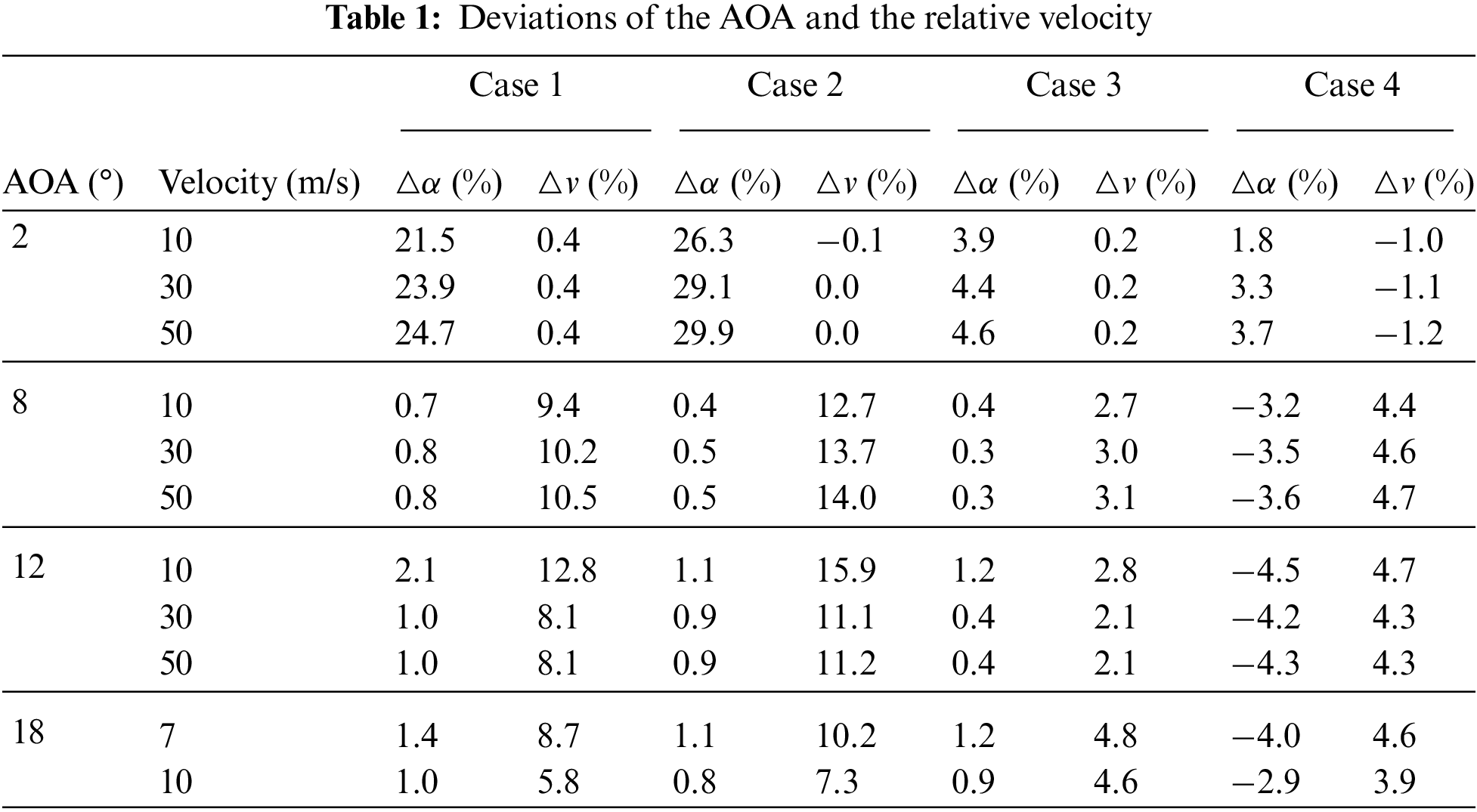
The deviations are shown in Table 1. The deviations of the AOA for case 3 and case 4 were both less than 5%, and were far less than those for the other two cases. The deviations of the relative velocity of the double-points cases were less than those of the single-point cases, which were still less than 5%. Therefore, case 3 was the best, followed by case 4.

3.1.2 Validation of Extraction Method

Johansen et al. [25] used the average azimuthal (AAT) method to extract the mean circumferential axial velocity and the tangential velocity from the CFD result. Then the two velocities were used to calculate the AOA according to the velocity triangle of the airfoil. Because the mean circumferential values were used, the AAT method was not suitable for the yawed case. Therefore, the curves of the AOA with the azimuth angle with the reference points method and the AAT method for the non-yaw condition were compared, as shown in Fig. 6. The α–Ψ curve with case 3 was very close to the results for the AAT method, and the α–Ψ curve with case 4 was larger than the first two curves. The variation trends for case 4 and case 3, however, were basically the same. Because the AAT method adopted the circumferential average values, the α–Ψ curve changed periodically with a frequency of 3 with a very small amplitude within a rotation cycle, whereas the α–Ψ curve with case 3 and case 4 decreased slightly when Ψ = 180°. This indicated the influence of the tower on the AOA.

Figure 6: α–Ψ curve at 75% r/R section at γ = 0°

3.2 Distribution of the AOA and the Relative Velocity

For the airfoil, the AOA and the Reynolds number (Re) determined the characteristics of the lift and the drag. For the blade, the chord length was the same at the same spanwise airfoil section of the blade. Re was related only to the relative velocity of a spanwise section, which was proportional to Re at different operating conditions. Therefore, the AOA and the relative velocity jointly determined the flow characteristics around the blades and the pressure distribution on the blade surfaces, thus affecting the power output and the aerodynamic load distribution of the wind turbine. In this study, the AOA and the relative velocity at the 25%–100% r/R spanwise sections of the b1 blade in a rotation cycle were extracted when the yaw angle was 0°, 15°, 30°, and 45°. Fig. 7 shows the distribution of the AOA and the relative velocity changes with the radius and the azimuth angle. For the non-yaw case, the two parameters were distributed in a circular pattern, indicating that the parameters only changed with the radius and had nothing to do with the azimuth angle. For the yawed case, the distributions no longer showed a circle, indicating that the AOA and the relative velocity were related to both the radius and the azimuth angle. According to the variation range of parameters in Fig. 7, with an increase in the yaw angle, the minimum value of the two parameters decreased, whereas the maximum value increased. In other words, the variation range of both the AOA and the relative velocity increased with an increase in the yaw angle.

Figure 7: Distribution of the AOA and the relative velocity for different yaw angles

To better observe the changing law of the AOA and the relative velocity with the radius and the azimuth, three sections were selected, which were the 25%, 65%, and 95% r/R spanwise sections of the b1 blade, representing the root, middle, and tip regions of the blade, respectively. The influences of the yaw angle on the AOA and the relative velocity were discussed.

Fig. 8a shows the α–ψ curves at different sections at different yaw angles. When γ was 0°, the AOA on all three sections changed very little with Ψ. When γ > 0°, the AOA had a periodic change of an approximate cosine curve during a rotation period. The α–ψ curves had the same changing law in the same cross-section. In the different sections, the changing trend was different, and the curve at the 25% r/R section was distributed essentially symmetrically on both sides of the 180° azimuth. With the azimuth angle changed from 0° to 360°, the α at the 65% and 95% r/R spanwise sections decreased first, then increased, and then decreased again. The maximum peak values of both curves were all between the 300° and 330° azimuths, and the minimum peak values were different from each other. At the 65% r/R sections, the minimum peak was around the 180° azimuth, whereas at the 95% r/R sections, the minimum peak was between the 120° and 150° azimuths.

Figure 8: The AOA and the relative velocity with the azimuth angle for different yaw angles

Fig. 8b shows the changing law of the relative velocity, which is denoted by the symbol vrel in the figure. vrel increased from the root region to the tip region of the blade. The changing law at the three sections was basically the same, and it changed according to the arccosine law. When Ψ was 180°, vrel had the maximum value, and the values on both sides had a basically symmetrical distribution. At the same cross-section, the larger the γ was, the larger the vrel variation was. At the same yaw angle, the relative fluctuation range of the 25% r/R section was the largest, whereas those of the 65% and 95% r/R sections decreased successively.

3.3 Analysis of Flow Characteristics

3.3.1 Pressure Distribution and Flow Field

Two yaw conditions of 15° and 45° were selected to analyze the influence of the yaw angle on the pressure distribution on the blade surface. As shown in Fig. 9, at the 25% r/R section, when γ = 15°, as Ψ increased, α decreased, and cp–x/c curves of the suction surfaces contracted inward, especially near the leading edge of the blade. The vertical distance between the upper and lower cp–x/c curves in the figure represents the effective pressure difference created by the lift at the corresponding chord location. With an increase in Ψ, α decreased, and the lift that was generated at this section decreased. When γ = 45°, as Ψ increased, α decreased as well. The changing amplitude of α at the 45° yaw was larger than that at the 15° yaw, which resulted in the cp–x/c curves of both the suction surface and the pressure surface contracting inward. Compared with the 15° yawed condition, the shape of the cp–x/c curve was significantly different.

The flow characteristics at the 25% r/R section at the 45° yaw were further analyzed with the flow lines around the airfoil. When Ψ = 0°, α was 16.9° which was the maximum AOA in all the calculated conditions. As shown in Figs. 9a and 10a, point A was the front stagnation point on the pressure surface. After bypassing the leading-edge point of the airfoil from point A, the air flowed backward along the suction surface, and point B was the peak point of the suction surface. After point B, the inverse pressure gradient increased sharply. The flow separation occurred on the leading edge of the airfoil. Then the flow reattached to the airfoil surface at point D. When Ψ = 60°, the leading-edge separation region decreased with the decreasing α, which was the process of B→C shown in Figs. 9b and 10b. The leading-edge separation was not observed when Ψ = 90°. When Ψ = 120°, α decreased continuously, and the cp–x/c curves of the suction surface and the pressure surface both contracted (as shown in Figs. 9c and 10c). When Ψ = 180°, α continued to decrease and became negative. The front stagnation point A moved from the pressure surface to the suction surface. The airflow bypassed the leading edge from point A and accelerated along the pressure surface continuously until it reached point B, where the pressure reached the minimum value of the whole airfoil surface. With the influence of the airfoil shape, the pressure on the suction surface was less than that on the pressure surface after point C, and the pressure on the upper and lower airfoil surfaces reversed after point D, but the values were basically the same. For this case, the pressure on the suction surface was greater than that on the pressure surface, and the torque generated was negative. The direction of the differential pressure pointed toward the pressure surface at the front part of the airfoil (before C), toward the suction surface at the middle part of the airfoil (from C to D), and toward the pressure surface again at the rear part of the airfoil (after D). Obviously, compared with the other conditions under which the directions of the differential pressure all pointed toward the suction surface, the aerodynamic force created at the 25% r/R spanwise section at 45° yaw and the 180° azimuth angle posed a greater threat to the structural safety of the blades. In addition, as the blade rotated, the separation vortex at the blade root region appeared and disappeared alternately, which caused the blade root region to have stronger dynamic characteristics and greater load fluctuation.

Figure 9: The pressure coefficient curves at different interfaces

Figure 10: The streamline around the airfoil at a 45° yaw angle

In Figs. 9e and 9f, at the 65% and 95% r/R spanwise sections, the suction peak value, pressure peak value, and the surface created by the cp–x/c curve indicated that the amounts of lift all decreased with the decrease of α. From the root region to the tip region of the blade, the influence of the yaw angle on cp–x/c curves decreased, and the change at the root region was the largest.

3.3.2 Flow Mechanism Analysis

According to this analysis, the changing law of the lift force at the different spanwise sections was consistent with the changing law of the AOA. The AOA, however, was not the only factor that affected the lift force. As shown in Fig. 9, for some conditions, the AOA was not the same, but the shape of the cp–x/c was very close. The reason for this change was that the magnitudes of the lift and the torque were also related to the Re. When α was the same, the lift increased with Re before a stall. For example, at the 95% r/R spanwise section and 15° yaw, the AOA of the 0° azimuth was greater than the AOA of the 180° azimuth, whereas the Re was the opposite. The effect of the reduced Re on the lift partially offset the effect of the AOA on the lift, making the cp–x/c curves of the two states almost coincide.

Compared with other working conditions, the same phenomenon existed. At the 25% r/R spanwise section and a 0° azimuth, the AOA for the 45° yaw was greater than that for the 15° yaw, but the Re for the 45° yaw was much smaller than that for the 15° yaw. At the same time, the leading-edge flow separation increased the suction surface pressure, so the lift for the 45° yaw was smaller instead. In general, the AOA and Re both affected the blade surface pressure distribution, but the AOA had a greater influence.

Through the above analysis, it could be seen that even at the 45° yaw, the flow separation of the leading edge at the blade root region was only found at the 0°–60° azimuth. Large-scale and destructive flow separation did not occur. This might have been due to the following reasons:

1.    The influence of the airfoil. The airfoil of the blades used in this study had smaller leading-edge radius, thickness, and camber, which were different from those of the National Renewable Energy Laboratory (NREL) Phase VI wind turbine (an S809 airfoil with a larger thickness was used) that often have been analyzed in the literature. The large-scale flow separation occurred at the airfoil trailing edge of the NREL Phase VI wind turbine at the rated condition. The separation of the laminar boundary layer near the leading edge with the action of a large adverse pressure gradient usually occurred in the airfoil in this study. When the adverse pressure gradient decreased, the flow became turbulent and then re-attached to the blade surface.

2.    The influence of the dynamic stall. The critical AOA in the yawed condition changed periodically, making the critical AOA for the dynamic stall much larger than the critical AOA of the 2D static stall. This effect gradually increased from the tip region to the root region of the blade. When the AOA at the root region reached its maximum value, the vortex did not propagate from the leading-edge area along the upper surface of the airfoil to the trailing edge and the airfoil did not enter a deep stall.

3.    The influence of Re. At the 45° yaw and the 0° azimuth, although the AOA was the largest, it could be seen from Fig. 8b that the relative velocity was the smallest at that time. The smaller relative velocity eased the flow and made the flow re-attach to the blade surface again after the leading-edge separation generated by a large adverse pressure gradient.

4.    The influence of the working condition. The rated working condition in this study was examined. Theoretically, when the velocity of the free stream increases, the separation increases as a result of the increase of the AOA.

4  Conclusion

In this study, the distributions of the AOA and the relative velocity, as well as the flow characteristics of the S-airfoil wind turbine for yaw cases, were analyzed according to the CFD method. The flow mechanism on the blade surface was discussed further. The conclusions were as follows:

1.    In a rotation period, the AOA and the relative velocity of the spanwise sections changed with the increase of the azimuth angle according to the law of cosines and anti-cosines. The larger the yaw angle was, the larger the fluctuation amplitude was. From the root region to the tip region of the blade, the fluctuation amplitude decreased gradually.

2.    In the yawed condition, the AOA and the Reynolds number affected the pressure distribution of the blade surface and the power output characteristics more. The influence of the AOA on the pressure distribution was greater than that of the Reynolds number. At the same time, the reverse change between the Reynolds number and the AOA reduced the influence degree of the AOA.

3.    With an increase in the yaw angle, the large fluctuation amplitude of the AOA appeared at the blade root region, resulting in a vortex that appeared and disappeared continuously at the leading edge of the suction surface of the blade. Because of the influence of the airfoil shape, the Reynolds number, and the working conditions, the separation did not propagate along the chord to the trailing edge of the blade, but the flow state of the suction surface still showed obvious dynamic characteristics.

The research results described in this paper could provide theoretical guidance for the development of flow control methods on the blade surface of a wind turbine, especially on the surface of the blade root in the yawed condition, to reduce the influence on the power loss and the power fluctuation of a wind turbine.

In this research, only the rated condition was studied. In the follow-up work, the yawed condition for different wind speeds and tip speed ratios will be analyzed, to obtain more comprehensive and instructive conclusions.

Acknowledgement: We thank LetPub (https://www.letpub.com) for its linguistic assistance during the preparation of this manuscript.

Funding Statement: The authors received no specific funding for this study.

Conflicts of Interest: The authors declare that they have no conflicts of interest to report regarding the present study.

This work is licensed under a Creative Commons Attribution 4.0 International License, which permits unrestricted use, distribution, and reproduction in any medium, provided the original work is properly cited.