Energy Engineering

DOI: 10.32604/ee.2022.019284

ARTICLE

A Novel Aquila Optimizer Based PV Array Reconfiguration Scheme to Generate Maximum Energy under Partial Shading Condition

Dong An1, Junqing Jia1, Wenchao Cai1, Deyu Yang1, Chao Lv1, Jiawei Zhu2 and Yingying Jiao3,*

1Inner Mongolia Power Research Institute, Huhhot, 010020, China
2School of Information Engineering, Chang’an University, Xi’an, 710064, China
3School of Information and Electrical Engineering, Shandong Jianzhu University, Jinan, 250101, China
*Corresponding Author: Yingying Jiao. Email: yingying.jiao@outlook.com
Received: 14 September 2021; Accepted: 24 February 2022

Nomenclature

1  Introduction

Recently, excessive energy demand has caused severe environmental deterioration and rapid energy exhaustion such as coal, oil, and natural gas, which requires a profound energy transformation due to the energy crisis [1–3]. In particular, solar energy is widely deemed as one desirable candidate, which has been widely employed in PV power generation [4–7]. Nevertheless, fixed free-standing PV systems are easily affected by various dynamic environmental conditions, which leads to mismatch loss and power loss, uneven irradiance and temperature, together with partial shading condition (PSC) [8–10]. Among them, PSC is mainly caused by clouds, trees, buildings, dust accumulation, bird droppings, and snow [11].

To solve these thorny obstacles caused by PSC, a wide range of solutions have been proposed such as installing bypass diodes in parallel on PV panel [12] and implementing maximum power point tracking (MPPT) techniques [13]. However, the connection of bypass diodes will engender power mismatch due to multi-peak characteristics in PV panels [12]. Meanwhile, MPPT technique is troublesome to apply in large-scale PV power stations because of the complicated execution and control cost [13].

Nowadays, PV array reconfiguration has been envisaged as a highly competitive strategy to harvest maximum power output under different PSCs, which basic principle is to rearrange the shadows in the same column of PV arrays through physical relocation (PR) [14], electrical rewiring (ER) [15] and electrical array reconfiguration (EAR) [16] to equalize the effect of any concentrated PSC. PV array reconfiguration can generally be categorized into fixed and dynamic reconfigurations according to whether the electrical interconnection alters. Nowadays, plenty of static reconfiguration methods have been proposed based on PR, ER, or both, e.g., fixed reconfiguration [17], column index method [18], special connection method [19], and odd-even configuration [20]. The obvious determination of static reconstruction is that it cannot respond effectively to the dynamic changes of the shadow. On the contrary, dynamic reconfiguration can effectively cope with various shadows. Thus far, many topologies have been widely used on dynamic reconfiguration, like series-parallel, total-cross-tied (TCT) [21], Suduku, and so on.

In recent years, an optimal PV array reconfiguration (OAR) via various meta-inspiration algorithms is proposed, such as genetic algorithm (GA) [22], particle swarm optimization (PSO) [23], ant colony algorithm (ACO) [24], grasshopper optimization algorithm (GOA) [25], and butterfly optimization algorithm (BOA) [26], which can seek the optimal power output from multiple MPPs under unequal solar irradiation for TCT topology. However, these meta-inspiration algorithms tend to easily fall into the low-quality local optimum due to inherent defects of strong randomness.

Therefore, this work devises a new Aquila optimizer (AO) to extract the maximum power of PV power plants under PSC in real-time. For validation, a complete 15 × 15 TCT PV array reconfiguration model is implemented and tested in simulation. The main novelties of this work are outlined as follows:

● An AO based real-time maximum power harvesting strategy from PV arrays under PSC by reconfiguring PV arrays is proposed.

● Compared to the original AO [27], the proposed approach carries out a series of discrete operations to address the discrete problem of PV array reconfiguration, which considerably enhances its application feasibility in solving any discrete optimization problem.

● 10 cases under PSCs are designed to simulate possible shadows caused by clouds, trees, buildings, dust accumulation, bird droppings, and snow. Besides, the effectiveness of AO on PV array reconfiguration is tested under such 10 shadows.

The rest sections are organized as follows: Section 2 presents the mathematical model of TCT PV array reconfiguration; Section 3 introduces AO and the discrete design of AO; Section 4 provides the design of AO based OAR; Section 5 shows the results and discussion of simulation; and Section 6 gives the conclusions.

2  TCT PV Array Reconfiguration Modelling

2.1 TCT-Connected PV Arrays

TCT-connected PV arrays are connected in parallel in each row, while these rows are connected in series. Because the voltages at both ends of each row are equal, the entire output voltage of the PV array is able to be modeled as

VD=∑p=1FVap(1)

where Vap is the maximum voltage of array at the pth row.

The law of Kirchhoff current indicates that the whole current flowing through each column of PV arrays can be described as

ID=∑q=1F(Ipq−I(p+1)q)=0,p=1,2,…,9,A,…,F(2)

where Ipq means output current across the pth row and the qth column of PV array.

2.2 Performance Evaluation

To evaluate the performance of OAR under PSC using AO, three indices (fill factor, mismatched power loss, and efficiency) are introduced, as follows:

Fill factor (FF): which is represented as the ratio of maximum output power under PSC (PPSC) to the product of the open-circuit voltage (VOC) and short circuit current (ISC).

FF=PPSCVOC×ISC(3)

Mismatched Power Loss (ΔPMMPL): which is described as the difference between maximum output power under the standard condition (PSTC) and PPSC. The standard condition is defined as the solar irradiation of 1000 W/m2 and the operation temperature of 25°C.

ΔPMMPL=PSTC−PPSC(4)

Efficiency (η%): which is defined as the ratio of PPSC to PSTC, it can be calculated by

η(%)=PPSCPSTC(5)

3  Aquila Optimizer

AO is designed by simulating the natural behavior of Aquila in capturing prey. Aquila’s pointed hook-shaped beak and sharp claws can help them quickly catch all kinds of prey, such as hares, marmots, squirrels, and other ground animals. Most Aquila can choose the best hunting method ingeniously and quickly according to the situation.

3.1 Principle of Aquila Optimizer

3.1.1 Solutions Initialization

Initial population of AO is randomly produced within the upper bound (UB) and lower bound (LB) according to the specific questions. It can be described by

Xij=rand×(UBj−LBj),i=1,2,…,Nj=1,2,…,Dim(6)

where Xij means the ith candidate solution with dimension j; N is population number; Dim is the dimension of the specific question; rand means a random number; LBj and UBj denote to the jth lower bound and upper bound, respectively.

3.1.2 Mathematical Model of Aquila Optimizer

AO modeling is mainly realized by simulating Aquila’s behavior when they are hunting: (1) choosing the searching area through high soar with the vertical stoop, (2) exploring in different searching spaces through contour flight with quick glide attack, (3) exploiting in convergence searching area through low flight with slow attack, and (4) swooping through the walk and grabbing prey. AO can switch between exploration and exploitation based on the condition: t≤23×T.

Step 1: Expanded exploration (X1)

Aquila explores widely the searching area by high soar, as shown in Fig. 1a. This behavior is expressed as

X1(t+1)=Xbest(t)×(1−tT)+(XM(t)−Xbest(t)×rand)(7)

where t means the current iteration and T denotes the total iterations; X1(t+1) denotes the solution at the (t+1)th iteration; Xbest(t) means the highest-quality solution gained during the tth iteration; rand randomly chooses from [0,1]; XM(t) represents the mean value of current solutions at the tth iteration, which is written by

XM(t)=1N∑i=1NXi(t)(8)

Step 2: Narrowed exploration (X2)

AO explores the area where the target prey appears to be ready for attacking, as described in Fig. 1b. This behavior is presented as

X2(t+1)=Xbest(t)×Levy(D)+XR(t)+(y−x)×rand(9)

where X2(t+1) indicates the solution at the (t+1)th iteration; XR(t) selects randomly from [1, N] at the tth iteration; D means the dimension of search space; and the function that expresses levy flight distribution is written by

Levy(D)=s×u×σ|v|1β(10)

where s = 0.01, u and v denote random numbers between 0 and 1. σ is calculated by

Figure 1: The behavior of the Aquila: (a) High soar with the vertical stoop; (b) Contour flight with quick glide attack; (c) Spiral shape; (d) Low flight with a slow attack; (e) Walk and grab prey; (f) The effects of the quality function (QF), G1, and G2 on the behavior of the AO

σ=(Γ(1+β)×sin⁡(πβ2)Γ(1+β2)×β×2(β−12))(11)

where β = 1.5, x and y that expresses the spiral shape in the search are expressed as

y=r×cos⁡(θ)(12)

x=r×sin⁡(θ)(13)

where

r=r1+U×D1(14)

θ=−ω×D1+θ1(15)

θ1=3×π2(16)

where r1 is a value between 1 and 20, which is used to fix the number of searching cycles; U = 0.00565. D1 is integer number; and ω = 0.005. The spiral behavior of AO is shown in Fig. 2c.

Step 3: Expanded exploitation (X3)

AO exploits the range where preys appear, and then approaches and attacks it, as shown the Fig. 1d. This behavior is presented as

X3(t+1)=(Xbest(t)−XM(t))×α−rand+((UB−LB)×rand+LB)×δ(17)

where X3(t+1) means the solution at the (t+1)th iteration; α and δ are the parameters used to adjust exploitation (α = δ=0.1).

Step 4: Narrowed exploitation (X4)

Fig. 1e describes the behavior that AO attacks the prey in the last location, which is presented as

X4(t+1)=QF×Xbest(t)−(G1×X(t)×rand)−G2×Levy(D)+rand×G1(18)

where X4(t+1) is the solution of the (t+1)th iteration; QF is applied to balance search methods, which is written by Eq. (19); G1 generated by Eq. (20) denotes various motions that Aquila tracks the target in the process of exploitation; G2 produced by Eq. (21) denotes the flight slope that Aquila tracks the target in the process of exploitation; X(t) is the current solution at the tth iteration; Fig. 2f provides the influences of QF, G1, and G2 on the behavior of the AO.

QF(t)=2×rand−1t(1−T)2(19)

G1=2×rand−1(20)

G2=2×(1−tT)(21)

Figure 2: The irradiation distribution of the 15 × 15 PV arrays under 10 cases of PSCs

3.2 Discrete Design of Aquila Optimizer

Reconfiguring PV arrays is a problem of discrete optimization. To apply the excellent optimization performance of AO for solving this problem, a series of discrete designs are performed on AO, as follows:

3.2.1 Discretization for Initial Population

Obviously, the method of population initialization shown in Eq. (10) is not suitable for PV array reconfiguration. Hence, An N matrix is introduced to represent the initial population of OAR modeling, which can be written as

N={[C]1,[C]2,[C]3,…,[C]npop}(22)

where C is a 15 × 15 matrix created by Eq. (23) to indicate the initial electrical connection state of PV arrays. npop is the number of population.

At the process of PV array reconfiguration, each PV array only exchanges with another PV array in the same column. Thus, the optimization variables should satisfy the following constraints:

{xpq∈{1,2,…,9,A,…,F},p=1,2,…,9,A,…,F;q=1,2,…,9,A,…,F∪p=0Fxpq={1,2,…,9,A,…,F},q=1,2,…,9,A,…,F(23)

where xpq denotes the electrical connection state of PV arrays at the pth row and the qth column. To satisfy the constraints in Eq. (22), a Matlab function ‘randperm (n)’ is introduced, as follows:

{Cq=randperm(15),q=1,2,…,9,A,…,FC=[C1,C2,…,Cq,…,C9,CA,…,CF](24)

where ‘randperm (15)’ means to randomly sort 15 data in a column; Cq represents the qth column of the C.

3.2.2 Discretization for Optimization Process

AO switches between exploration and exploitation according to the situation to choose the best hunting method ingeniously and quickly. To make the optimization method suitable for PV array reconfiguration, the sequence of solutions optimized by Eqs. (7)–(21) will be chosen to reassign the electrical connection state of each column of PV arrays, as follows:

spq=rank(xpq,xq)(25)

where xq=[X1,X2,…,Xi,…,X9,XA,…,XF] is the solution vector of arrays at the qth column; rank(xpq,xq) denotes the order of xpq among all solutions xq, which is designed in ascending order.

4  Design of Aquila Optimizer Based OAR

Since the physical position of all arrays in TCT configuration is fixed, an OAR model via electrical switches is introduced to reconfigure the position of arrays. Firstly, a discrete design for AO is performed for OAR model to obtain the optimal electrical connection state. After that, the physical position of PV arrays is rearranged via electrical switches in conformity with the obtained electrical connection state.

4.1 Objective Function

The primary goal of PV power plant is to extract the maximum output power under PSC, and its objective function is expressed as

f=maxP(C)=max(n×ID(C)×VD(C))(26)

where P(C) is the output power of the testing PV power plant at the Cth case of PSC; n is the number of sub-systems of the testing PV power plant.

4.2 Execution Procedure

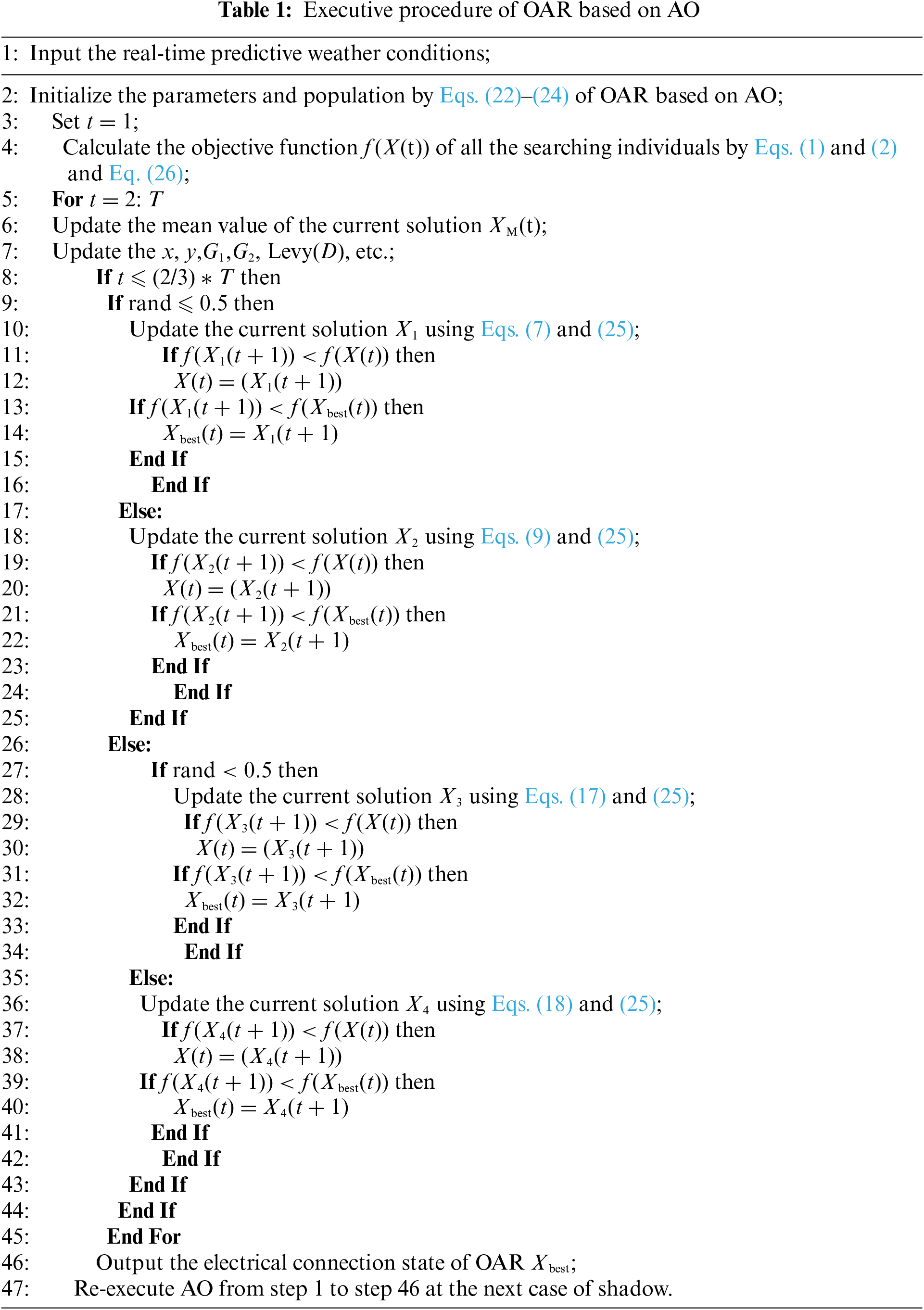
On the whole, the entire executive procedure of OAR based on AO is provided in Table 1.

5  Case Studies

5.1 Operating Conditions Setting

In this work, AO is applied to a test PV power station under 10 cases of PSCs (see Fig. 2) to validate its application reliability. PV power station is composed of 20 identical subsystems while each subsystem is formed by 15 × 15 TCT arrays. Note that the 10 cases of PSCs are based on the simulation of shading effects caused by clouds, trees, buildings, dust accumulation, bird droppings, and snow, in which different color blocks represent different irradiation intensity, i.e., white block is 1000 W/m2, pale-yellow block is 900 W/m2, light blue block is 800 W/m2 and others shown in Fig. 2. Table 2 gives the electrical characteristics of each PV array. Moreover, five algorithms (e.g., GA [22], PSO [23], ACO [24], GOA [25], and BOA [26]) are used for performance comparison with that of AO. T and N of all algorithms are unified to be 200 and 50, respectively to guarantee a fair and reliable comparison. Because the proposed method is based on meta-heuristic algorithm, each run will inevitably produce different results. To avoid this drawback to the greatest extent and obtain the global optimal solution, 30 runs of AO are undertaken on Matlab/Simulink 2017b using a personal computer with an Intel(R) Core (TM) i5-8400 CPU @ 2.80 GHz and 12 GB RAM. The applied solver is ode23 with the variable-step size of 10-3 s.

5.2 Result Analysis

Table 3 provides the optimization results of OAR under 10 cases of PSCs in 30 runs of six algorithms. Here, Pmax and Pmean are the maximum and mean values of output power in 30 independent runs. From Table 3, it can be seen that AO acquires the optimal Pmax and Pmean (in bold). In addition, three evaluation indices (FF, ΔPMMPL and η) are introduced to further validate the performance of AO. The calculation of the three indicators depends on the total Pmean of 10 cases of PSCs. One can see clearly that AO can get the largest FF and η as well as the smallest ΔPMMPL compared with other five algorithms. Particularly, FF and η obtained by AO are 1.67% and 1.68% higher than those of BOA, respectively, while ΔPMMPL has a 4.34% decrease.

The optimal solution of the 15 × 15 PV arrays reconfigured by AO is provided in Fig. 3, where concentrated shadows of all PV arrays in Fig. 2 are re-distributed to different rows. It dramatically increases the output power of PV plants. Neglecting the voltage drop of bypass diode, the maximum output power obtained by AO under the 4th case of PSC is 28.08% higher than that without optimization, as described in Fig. 4. Furthermore, the number of power peaks in the P-V curve can be significantly reduced by using AO. Fig. 5 gives the convergence result of the AO algorithm for 15 x 15 PV arrays at the 4th case of PSC. It can be seen that AO can quickly converge to a high-quality optimal solution.

Figure 3: Optimal solution of the 15 × 15 PV arrays reconfigured by AO with 10 cases of PSCs

Figure 4: Comparison result of the sub-system acquired by without optimization and AO at the 4th case of PSC. (a) I-V curves, and (b) P-V curves

Figure 5: The convergence diagram of the AO for 15 × 15 PV arrays at the 4th case of PSC

6  Conclusions

An AO based OAR is proposed for real-time maximum power extraction under PSC of PV arrays in this work, which contributions are drawn as follows:

(1) AO contains a series of discrete operations during optimization to solve the discrete problem of PV array reconfiguration, which owns great potential to apply in other complex discrete optimization problems.

(2) This work comprehensively considers the impact of PSC caused by clouds, trees, buildings, dust accumulation, bird droppings, and snow for PV array and simulates the 10 cases of PSCs based on this impact to validate the application reliability of AO under various PSCs.

(3) A series of experiments based on 10 cases of PSCs are designed to validate the optimization performance of AO compared against five well-known algorithms (e.g., GA, PSO, ACO, GOA, and BOA). Simulation results indicate that the mismatched power loss obtained by AO is the smallest, which can be decreased by 4.34% against BOA. Furthermore, it can be seen that the number of multiple peaks caused by the various PSCs can be significantly reduced by AO.

Future studies will focus on the following aspects:

(1) Apply the proposed AO based OAR to larger-scale PV arrays.

(2) Apply discrete AO to solve other discrete optimization problems.

Funding Statement: This work is supported by the Scientific Research Projects of Inner Mongolia Power (Group) Co., Ltd. (Internal Electric Technology (2021) No. 3).

Conflicts of Interest: Authors Deyu Yang, Junqing Jia, Wenli Wu, Wenchao Cai, Dong An are employed by Inner Mongolia Power Research Institute. The remaining authors declare that the research was conducted in the absence of any commercial or financial relationships that could be construed as a potential conflict of interest.

This work is licensed under a Creative Commons Attribution 4.0 International License, which permits unrestricted use, distribution, and reproduction in any medium, provided the original work is properly cited.