Energy Engineering

DOI: 10.32604/ee.2022.014816

ARTICLE

Power Quality Assessment Based on Rough AHP and Extension Analysis

Guofeng Liu*, Can Zhang, Zhengyi Zhu and Xuyan Wang

State Grid Nanjing Power Supply Company, Nanjing, 210019, China
*Corresponding Author: Guofeng Liu. Email: lgfsgn@sina.com
Received: 01 November 2020; Accepted: 10 December 2020

Nomenclature:

1  Introduction

Scientific and reasonable comprehensive assessment of power quality of smart grid is the basis for restraining and urging power companies and power users to jointly maintain the power quality environment of public power grid, and is also the main basis for measuring power quality and formulating electricity price, which has profound theoretical and practical significance [1,2]. At present, the comprehensive judgment methods of power quality are mainly based on fuzzy mathematics [3], probability statistics and vector algebra method [4,5], evaluation method based on grey theory [6,7], evaluation method based on subjective and objective weights [8–10], grey cloud evidential reasoning [11], variable fuzzy set [12] and random forest [13].

In the process of evaluation, the above methods are uncertain to a certain extent or too subjective. For example, in reference [3], the concept of interval average distribution density is used to establish a fuzzy model for power quality evaluation, but a single subjective weighting method is used to determine the weight value, which has a great impact on the accuracy of power quality assessment results; according to the main characteristics of each single power quality index in reference [5], vector algebra method is used to normalize and quantify them effectively. However, selecting different reference values will produce different evaluation results, which is not conducive to the objective evaluation of power quality. The power quality assessment method based on genetic projection pursuit can extract the characteristics of high-dimensional nonlinear evaluation indexes by automatic search, which overcomes the defects of human subjective factors in traditional evaluation methods. However, due to the concealment in its own evaluation process, it increases the uncertainty of evaluation results.

The combination of rough sets theory [14–16] and analytic hierarchy process (AHP) [17] can overcome the shortcomings of classical AHP and has been applied in many practical applications. Lee et al. [18] used rough set theory and group AHP for the evaluation of new service concepts and considerable results have been achieved. Zhang [19] studied rough set and AHP which was significant for the risk assessment of maintenance. Sun et al. [20] evaluated the performance of combined cooling heating and power (CCHP) system based on interval rough number AHP. Peng et al. [21] carried out the transformer state assessment based on rough sets theory and AHP. Wan et al. [22] adopted rough set and fuzzy AHP to determine customer demand weight. Extension analysis can solve the problem of incompatibility of various features of things [23–29]. Liu et al. [23] built the matter element extension model for risk analysis of buried crude oil pipeline. Zhai et al. [24] combined set pair analysis and extension theory coupling model and applied them for river health evaluation. Zhou et al. [25] proposed an improved extension AHP to evaluate the power failure. Jiang et al. [26] put forward a risk assessment approach of highway tunnel construction based on analytic hierarchy process and extension model.

In view of the shortcomings of the above methods, rough sets theory is introduced to improve the classical AHP when determining the weight of indicators in the power quality assessment indicator system and a rough AHP is proposed to aggregate the weight information of multiple experts, so as to eliminate the subjective influence of a single expert. Based on the characteristic of extension analysis for solving the problem of incompatibility of various features of things, extension analysis method is adopted to assess the power quality.

2  Framework

2.1 Power Quality Assessment Indicator System

In this paper, six power quality standards of national grid are used as the basis of comprehensive assessment of power quality, and each power quality standard is taken as assessment indicator. The six assessment indicators of power quality are frequency deviation, total harmonic distortion rate of voltage, voltage fluctuation, voltage flicker, voltage deviation and voltage three-phase unbalance degree, which are expressed by I1-I6, respectively. They are divided into several quality grades which are expressed by D1–Dh, respectively. The power quality assessment indicator system is shown in Fig. 1.

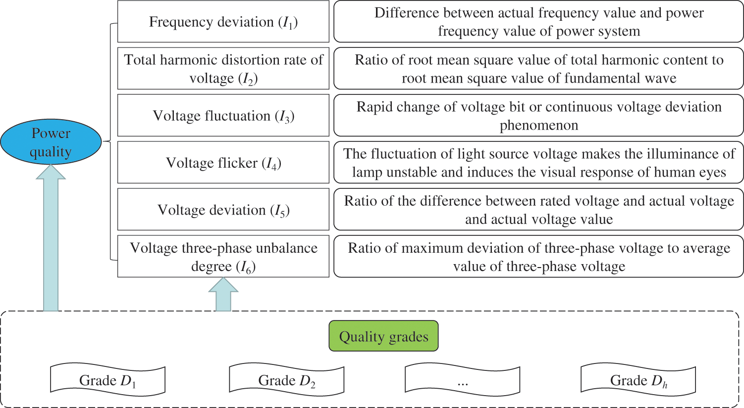
Figure 1: The power quality assessment indicator system

2.2 Research Framework

The overall research framework is shown in Fig. 2, which include three parts: the construction of assessment indicator system, the determination of assessment indicator weight and the assessment of power quality.

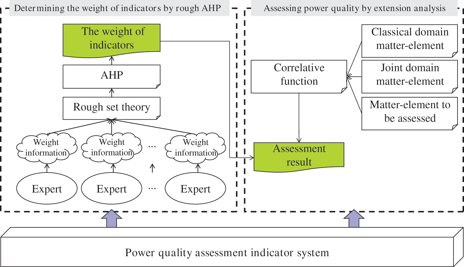
Figure 2: The research framework

The construction of assessment indicator system is given in the above section. The other parts are explained in Fig. 2. The method and theoretical innovations are mainly elaborated as follows:

(1)   In the determination of assessment indicator weight, multi-expert comprehensive judgment is adopted for eliminating the adverse effects of single expert judgment, rough sets theory is introduced to aggregate the judgment opinions of all experts, and the weights of the indicators is calculated by AHP.

(2)   In the assessment of power quality, the classical domain matter-element, joint domain matter-element and matter-element to be assessed are obtained by extension analysis theory. Then based on correlation function both the assessment grade of total power quality and each assessment indicator can be obtained. According to the assessment result, the key factors affecting power quality will be analyzed.

3  Method

3.1 Determining the Weight of Indicator by Rough AHP

AHP method [17] was put forward by Thomas L. Saaty. This method can not only make clear the hierarchical structure of the components of complex problem, but also verify the consistency of the results. Therefore, it has been widely applied in the weighting of multi-attribute decision-making problem [30,31]. Experts inevitably have subjectivity in judging the relative importance of indicators. To a certain extent, the adverse effects of single expert judgment can be eliminated by using multiple experts for comprehensive judgment. The judgment of relative importance between indicators by multiple experts is obviously indistinguishable when aggregating the judgment opinions of all experts. Instead of a membership function, the concept of rough boundary interval in rough sets theory [14–16] can represent the indistinguishability as a set boundary area. It can better aggregate the judgment opinions of all experts. Accordingly, a rough AHP method is designed to determine the weight of indicators in power quality assessment.

3.1.1 Basic Concepts of Rough Sets

Here, U is used to represent a domain which is actually a nonempty finite set of objects. Y is any object in U.

Concept 1. Upper and lower approximation sets [14–16].

In U, all objects are divided into n partitions: S1, S2,…, Sn. If these n partition has the order of S1 < S2 <…< Sn, the upper and lower approximation sets of any partition Si (1≤i≤n) can be defined as follows:

AS¯(Si)={Y∈K|K⊆U/R(Y)∧K≥Si}AS¯(Si)={Y∈K|K⊆U/R(Y)∧K≤Si}(1)

where U/R(Y) represents the partition of the indistinct relationship R(Y) in U.

Concept 2. Rough boundary interval [14–16].

According to the above definition, any ambiguous partition Si in U can be represented by its rough boundary interval RN(Si). RN(Si) consists of its rough lower limit L_(Si) and rough upper limit L¯(Si) which are defined as follows:

L_(Si)=∑Y∈AS_(Si)R(Y)N_(Si)(2)

L¯(Si)=∑Y∈AS¯(Si)R(Y)N¯(Si)(3)

where N¯(Si) is the number of objects in the upper approximation set of Si and N_(Si) is the number of objects in the upper approximation set of Si.

As can be seen, an ambiguous partition in the domain can be represented by a rough boundary interval containing a rough lower limit and a rough upper limit as follows:

RN(Si)=[L_(Si),L¯(Si)](4)

3.1.2 Rough AHP

In the proposed rough AHP, the concept of rough boundary interval in rough sets theory is introduced in classical AHP to aggregate the judgment opinions of multiple experts. The detailed steps are as follows:

Step 1. Construct the comparison matrix.

According to the indicator system shown in Fig. 1, multiple experts compare the importance of each indicator under the constraint of the overall objective. Here, power quality is the overall objective. Let the overall objective be the criterion, and the indicators controlled by it is I1∼Im(m=6). The relative importance of indicator with regard to the overall objective is the weight of indicator. The weight is determined by pairwise comparison of 1–9 scales shown in Table 1.

Assuming that there are p experts, each expert carries out the pairwise comparison of the indicators by 1–9 scales. Then p pairwise comparison matrices are obtained. The pairwise comparison matrix given by expert t (t = 1, 2,…, p) is defined as follows:

Φt=[1ϕ12t⋯ϕ1mtϕ21t1⋯ϕ2mt⋮⋮⋮ϕm1tϕm2t⋯1](5)

Step 2. Consistency test.

For pairwise comparison matrix Φt, its consistency ratio is defined as follows:

CRt=CItRI(6)

where CIt=λmaxt−mm−1 is the consistency index of Φt, here λmaxt is the largest eigenvalue of Φt and m is the dimensionality of Φt; RI is the random index which is only related to the matrix dimensionality and can be obtained according to Table 2.

When CRt<0.1, the consistency of pairwise comparison matrix Φt is acceptable; when CRt=0.1 or CRt>0.1, the consistency of pairwise comparison matrix Φt is not acceptable and the matrix should be modified by the corresponding expert.

Step 3. Judgment aggregation by rough boundary interval.

Based on pairwise comparison matrices Φ1,Φ2,…,Φp given by p experts, the group decision matrix is constructed as follows:

Φ=[1ϕ12⋯ϕ1mϕ211⋯ϕ2m⋮⋮⋮ϕm1ϕm2⋯1](7)

where ϕkj={ϕkj1,ϕkj2,…,ϕkjp}(k,j=1,2,…,m and k≠j).

The rough boundary interval of ϕkjt∈ϕkj is obtained as follows.

RN(ϕkjt)=[ϕkjt,−,ϕkjt,+](8)

where ϕkjt,− is the rough lower limit of ϕkjt in set ϕkj and ϕkjt,+ is the rough upper limit of ϕkjt in set ϕkj.

Therefore, the rough boundary interval of ϕkj can be represented as follows:

RN(ϕkj)={RN(ϕkj1),RN(ϕkj2),…,RN(ϕkjp)}(9)

Based on the operational rule of rough boundary interval, the average form of RN(ϕkj) is obtained as follows:

ARN(ϕkj)=[ϕkj−,ϕkj+]=[∑t=1pϕkjt,−p,∑t=1pϕkjt,+p](10)

where ϕkj− is the rough lower limit of set ϕkj and ϕkj+ is the rough upper limit of set ϕkj.

The rough judgment matrix is constructed as follows:

EA=[1ARN(ϕ12)⋯ARN(ϕ1m)ARN(ϕ21)1⋯ARN(ϕ2m)⋮⋮⋮ARN(ϕm1)ARN(ϕm2)⋯1](11)

Step 4. Divide rough judgment matrix and solve the eigenvectors.

Rough judgment matrix EA is divided into EA− and EA+. Here, EA− is the rough lower limit matrix and EA+is the rough upper limit matrix. EA− and EA+are expressed as follows:

EA−=[1ϕ12−⋯ϕ1m−ϕ21−1⋯ϕ2m−⋮⋮⋮ϕm1−ϕm2−⋯1](12)

EA+=[1ϕ12+⋯ϕ1m+ϕ21+1⋯ϕ2m+⋮⋮⋮ϕm1+ϕm2+⋯1](13)

The eigenvectors corresponding to the maximum eigenvalues of EA− and EA+are obtained respectively as follows:

VA−=[va1−,va2−,⋯,vam−]T(14)

VA+=[va1+,va2+,⋯,vam+]T(15)

where vaj− are the value of VA− on dimension j and vaj+ are the value of VA+on dimension j, here j = 1, 2,…, m.

Step 5. Weight value calculation.

The weight value of indicator Ij is calculated as follows:

ωj=|vaj−|+|vaj+|2(16)

Lastly the weight vector is obtained as follows:

ω=[ω1,ω2,…,ωm]T(17)

3.2 Assessing Power Quality by Extension Analysis

Extension analysis theory can classify the assessment indicators of power quality from the dynamic and transformation perspective and quantitatively express the quality grade of the indicators by the value of correlation function. The calculation of correlation function is based on the actual measured objective data.

Concept 3. Matter-element [27–29].

According to the extension analysis theory, the matter-element to be assessed is expressed by R0. R0 is defined as an ordered triples: R0=(Y0,I,v0). Here Y0 represents the unknown assessment grade of R0, I={I1,I2,…,Im} is the indicator set which represents the characteristics of R0 and v0=[v1,v2,…,vm] is the corresponding indicator value vector. Therefore R0 can be expressed as follows:

R0=[Y0I1v1I2v2⋮⋮Imvm](18)

Concept 4. Classical domain [27–29].

The classical domain refers to the range of values specified by the corresponding characteristics of each assessment grade of the object to be assessed. The classical domain matrix can be expressed as follows:

Rl=[YlI1[al1,bl1]I2[al2,bl2]⋮⋮Im[alm,blm]](19)

where Yl (l = 1, 2,…, h) is the lth assessment grade of R0 and [alj,blj] is the indicator value interval corresponding to Yl on indicator Ij.

Concept 5. Joint domain [27–29].

The joint domain refers to the range of values specified by all assessment grades of the object to be assessed.The joint domain matrix can be expressed as follows:

R=[YI1[a1,b1]I2[a2,b2]⋮⋮Im[am,bm]](20)

where Y is the set of all assessment grades of R0 and [aj,bj] is the indicator value interval corresponding to all assessment grades on index Ij.

Concept 6. Correlation function [27–29].

Correlation function describes the mapping of elements in matter element to real axis, which is specifically expressed as the quantitative relationship between vj and two interval [alj,blj] and [aj,bj].Through the correlation function, we can describe quantitatively and objectively the degree and its change of an element belonging to a certain property. For the elements in the same domain, we can also divide the elements into different grades according to the value of the correlation function value.

The module of bounded interval x=[a,b] is defined as follows:

|x|=|b−a|(21)

The distance from point x0 to interval x=[a,b] is defined as follows:

ρ(x0,x)=|x0−12(a+b)|−12(b−a)(22)

Assuming that there are two intervals x1=[a1,b1] and x2=[a2,b2] and they satisfy that x1⊂x2, the correlation function is defined as follows:

K(x)={−ρ(x,x1)|x1|,x∈x1ρ(x,x1)ρ(x,x2)−ρ(x,x1),x∉x1(23)

The properties of correlation function K(x) are as follows:

(1)   When K(x)>1, it indicates that the assessment object exceeds the upper limit required.

(2)   When 0≤K(x)≤1, it indicates that the assessment object meets the requirement. The larger its value, the closer it is to the upper limit required.

(3)   When −1≤K(x)<0, it indicates that the assessment object does not meet the requirement, but has the condition that can be converted to meet the requirement.

(4)   When K(x)<−1, it indicates that the assessment object does not meet the requirement, and does not have the condition to convert to meet the requirement.

Here, let x=vj, x1=[alj,blj] and x2=[aj,bj], correlation function Kl(vj) describes the quantitative relationship from indicator value vj of matter-element R0 to be assessed to two intervals [alj,blj] and [aj,bj]. It represents the membership degree of matter-element R0 to be assessed with respect to assessment grade Yl on indicator Ij and is defined as follows:

Kl(vj)={−ρ(vj,[alj,blj])|[alj,blj]|,vj∈[alj,blj]ρ(vj,[alj,blj])ρ(vj,[aj,bj])−ρ(vj,[alj,blj]),vj∉[alj,blj](24)

Based on weight vector ω=[ω1,ω2,…,ωm]T obtained by Eqs. (16) and (17), the comprehensive correlation function value is obtained as follows:

Kl=∑j=1mωjKl(vj)(25)

If Kg=maxl=1,2,…,h⁡{Kl}, here g=1,2,…,h, the assessment grade of the power quality to be assessed is Dg.

4  Case Study

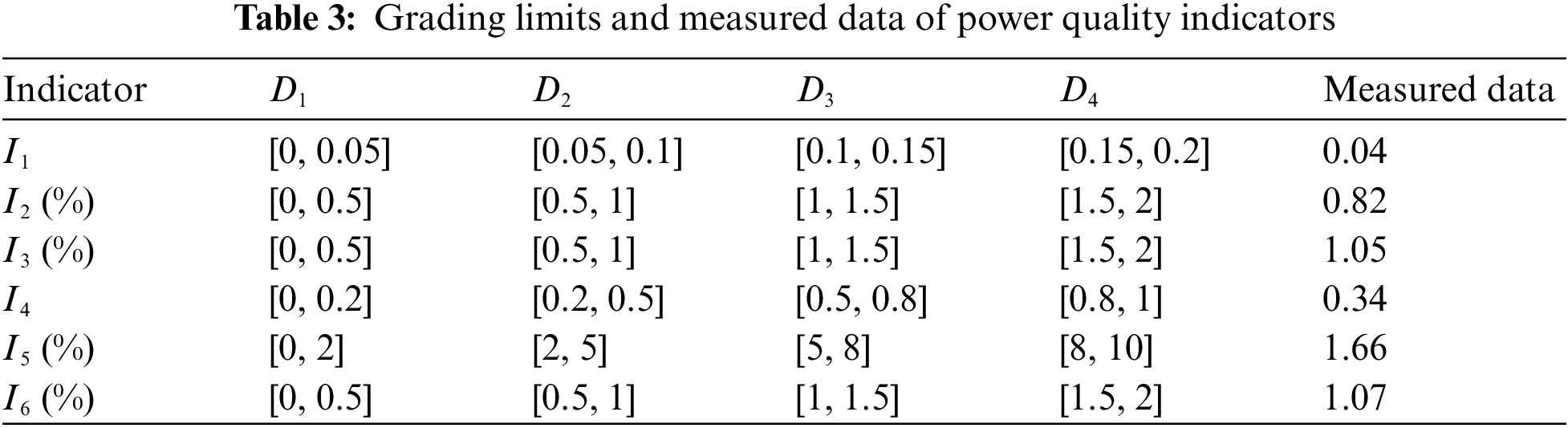
With the rapid development of economy and the gradual improvement of people's living standards, the power consumption of the whole society is increasing, and various new non-linear asymmetric electrical equipment have been widely used. A converting station in a wind farm of China is in line with these characteristics and is very representative in China. Therefore its 110 kV bus can be taken as research object to illustrate the feasibility of the proposed method. Its power quality is comprehensively assessed by the proposed method as follows. The power quality is divided into four quality grades: high quality, good, medium and qualified. They are expressed by D1–D4, respectively.

The grading limits and measured data of power quality indicators are shown in Table 3.

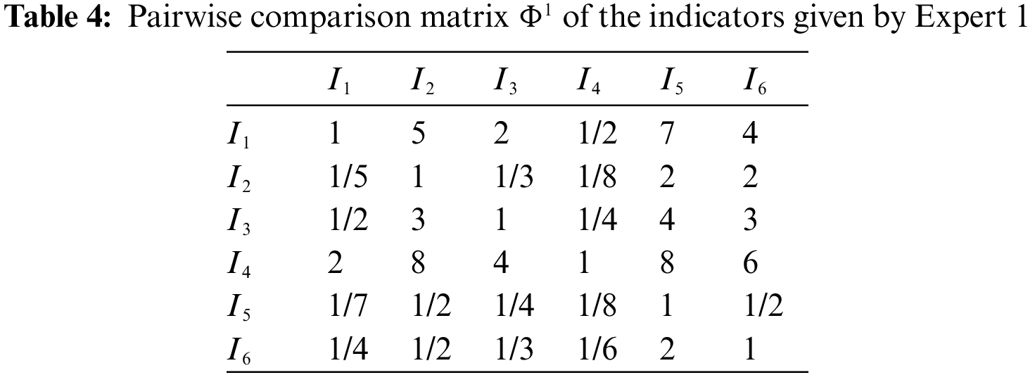
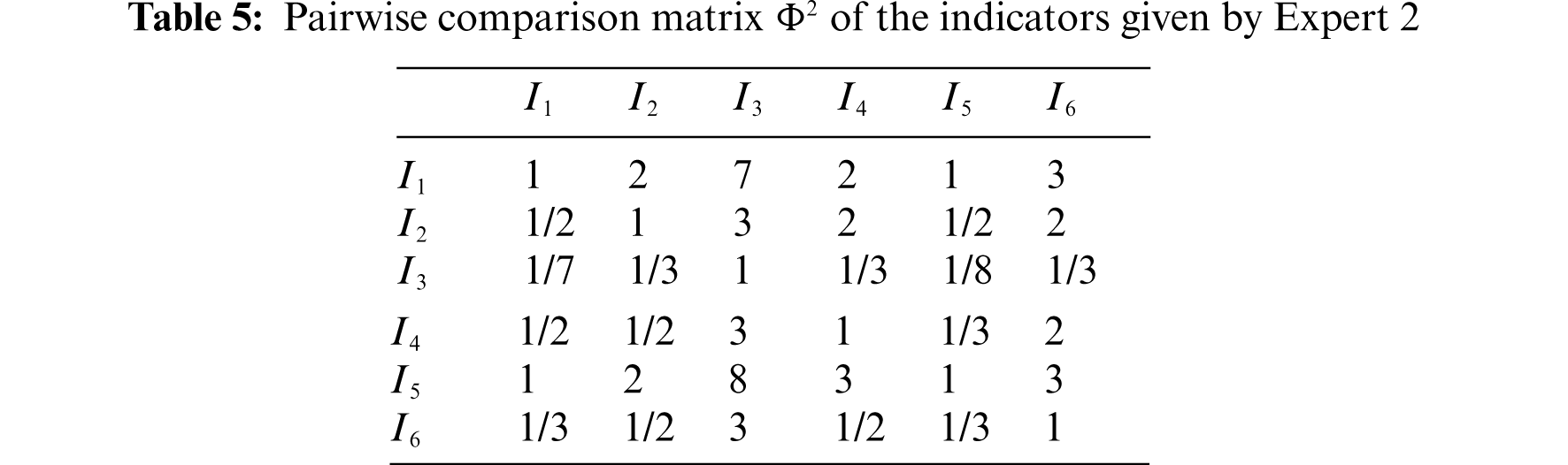
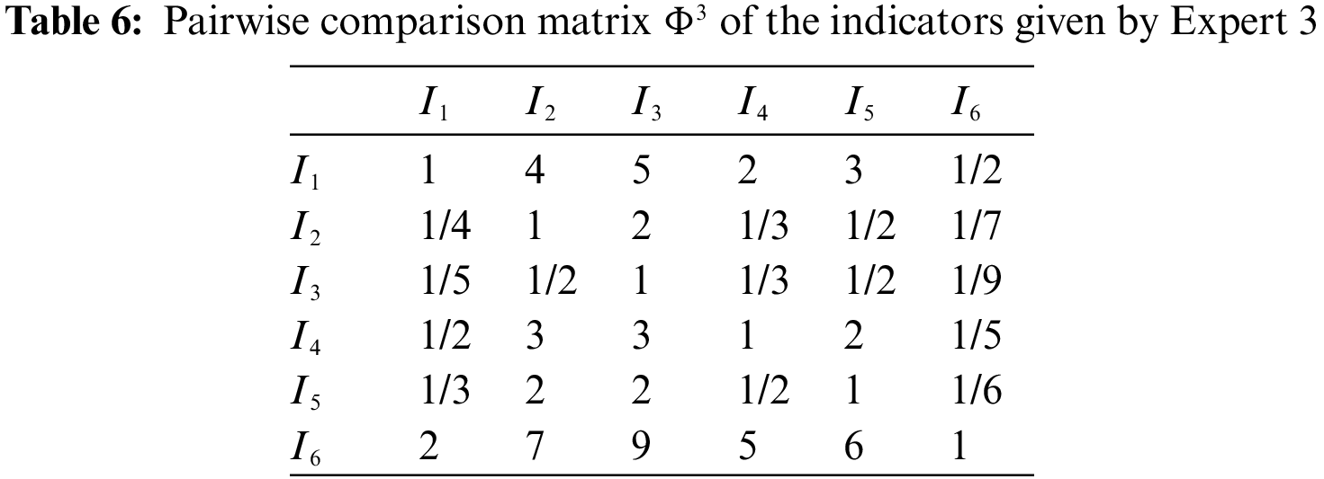
Firstly the weight of indicator is determined by the proposed rough AHP as follows. Assuming that there are three experts, each expert carries out the pairwise comparison of the indicators according to 1–9 scales in Table 1, then three pairwise comparison matrices are obtained as shown in Tables 4–6.

The consistency index and consistency ratio of the three pairwise comparison matrices is shown in Table 7.

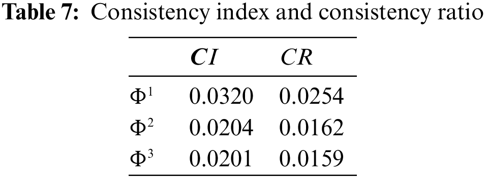
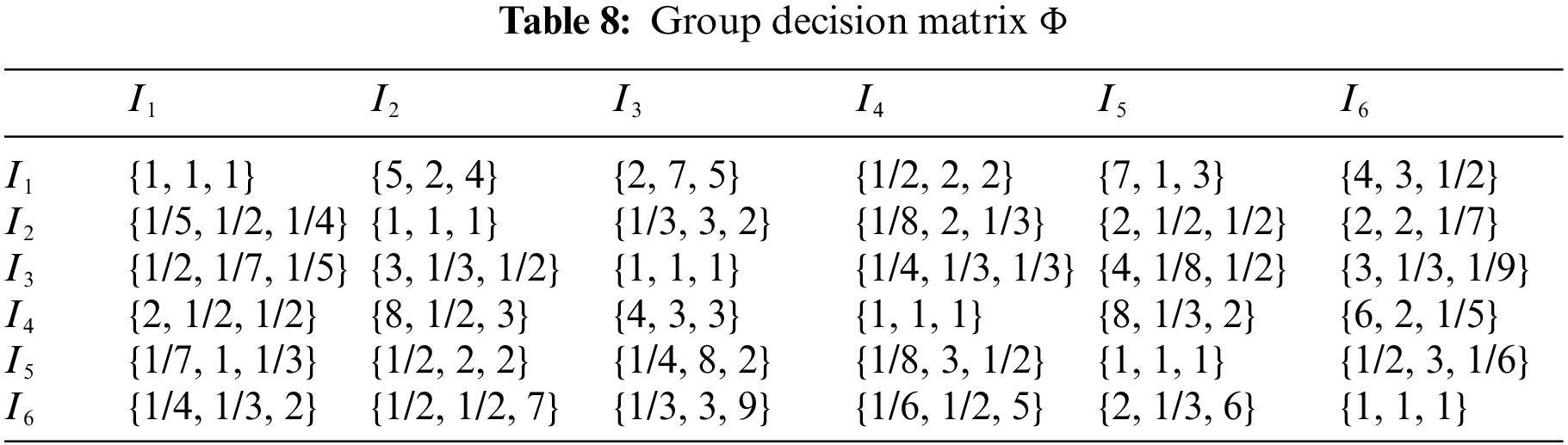
As can be seen, the consistency ratios of the three pairwise comparison matrices all have values less than 0.1, so the consistency of each pairwise comparison matrix is acceptable. Then according to Eq. (7) the group decision matrix is constructed as shown in Table 8.

Next ϕ12={5,2,4} is taken as an example to show the calculation process of rough boundary interval based on Eqs. (1)–(4). In ϕ12={5,2,4}, the lower and upper approximation sets of ϕ121=5 are {5, 2, 4} and {5}. Therefore, the rough lower limit of ϕ121 in set ϕ12 is ϕ121,−=5+2+43=3.6667, while the rough upper limit of ϕ121 in set ϕ12 is ϕ121,+=51=5. As a result, the rough boundary interval of ϕ121 is obtained as RN(ϕ121)= [3.6667, 5]. Similarly, the rough boundary intervals of ϕ122=2 and ϕ123=4 are obtained as RN(ϕ122)= [2, 3.6667] and RN(ϕ123)= [3, 4.5]. According to Eq. (10), the rough boundary intervals of ϕ12 is obtained as ARN(ϕ12)= [2.8889, 4.3889].

Then the rough judgment matrix is constructed as shown in Table 9.

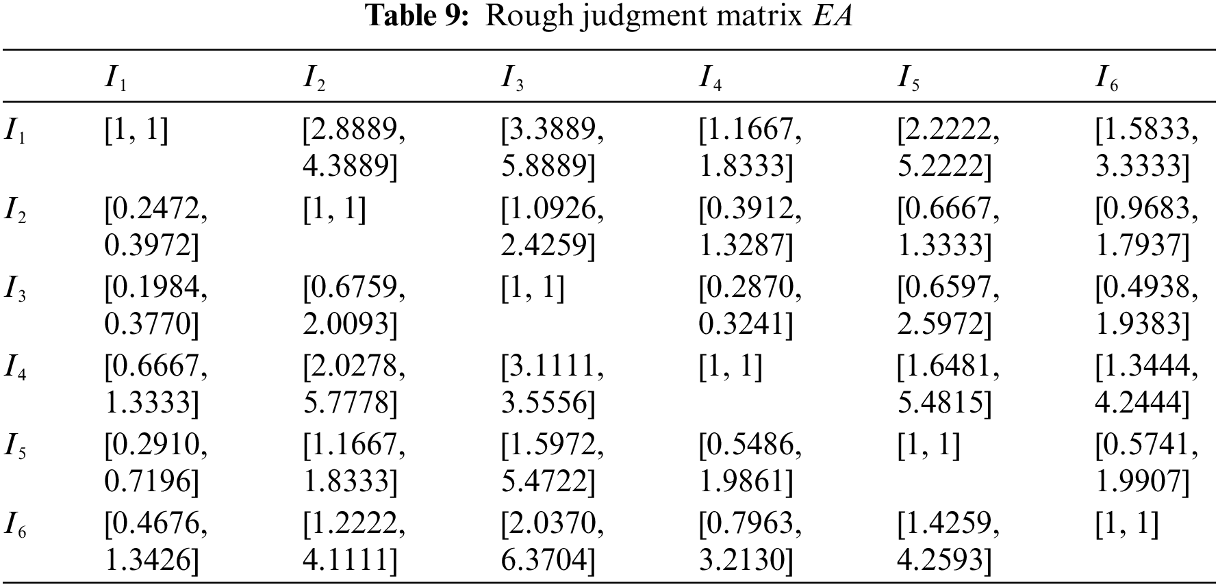
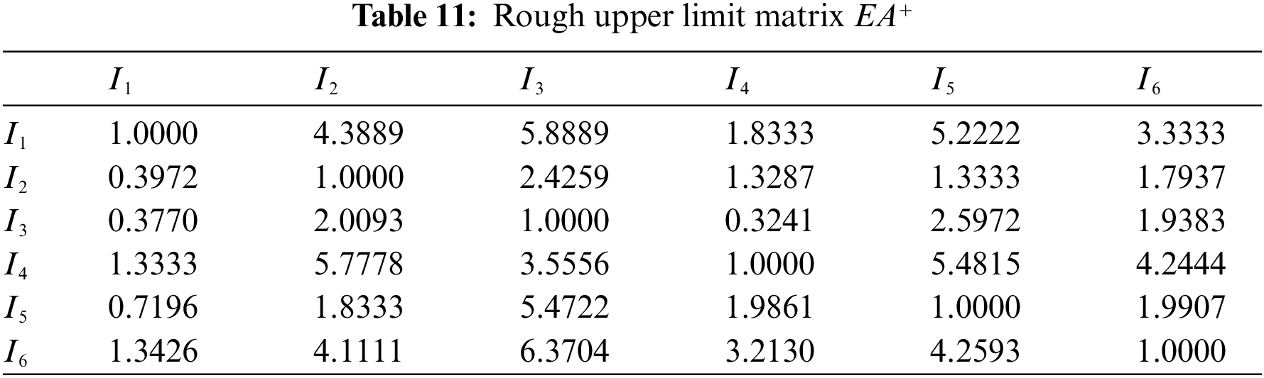
Rough judgment matrix EA is then divided into rough lower limit matrix EA− and rough upper limit matrix EA+ as shown in Tables 10 and 11.

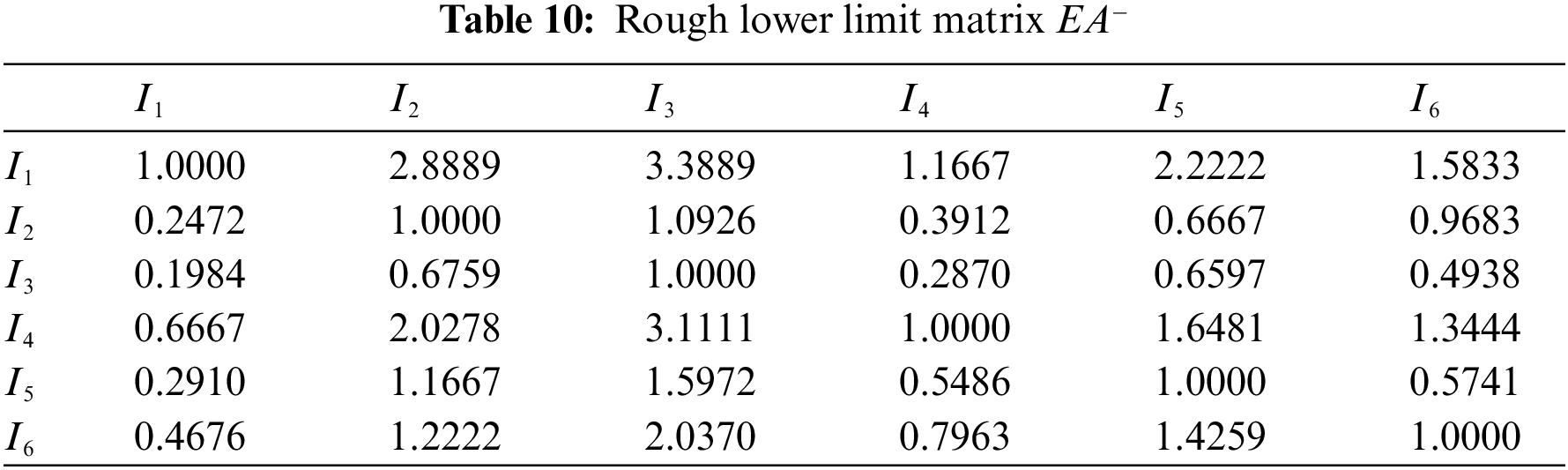
By Matlab, the eigenvectors corresponding to the maximum eigenvalues of EA− and EA+are obtained respectively as:

EA−= [0.6592, 0.2361, 0.1725, 0.5173, 0.2676, 0.3753]T;

EA+= [0.5274, 0.2218, 0.2110, 0.5332, 0.3221, 0.4901]T.

According to Eqs. (16) and (17), the weight vector is obtained as ω = [0.2617, 0.1010, 0.0846, 0.2317, 0.1301, 0.1909]T.

Based on weight vector ω and the grading limits and measured data shown in Table 3, the correlation function values are obtained as shown in Table 12 according to Eq. (24).

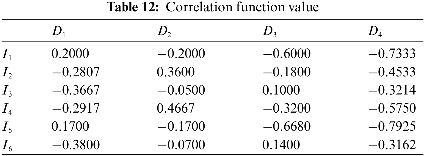
At last, the comprehensive correlation function values are obtained according to Eq. (25) as: K1=−0.1250, K2=0.0524, K3=−0.3011 and K4=−0.5616. Because K2=maxl=1,2,3,4⁡{Kl}, the power quality to be assessed belongs to assessment grade D2: good.

To demonstrate the validity and applicability, the assessment result of the proposed method is compared with the assessment result of D-S evidence theory [32]. By treating every indicator as evidence, the identification framework is built in which the assessment grades (D1–D4) are elements. Based on the indicator measured data in Table 3 and the weight vector obtained above, weighted evidence synthesis is carried out. The comparison of the assessment results are shown in Fig. 3.

From Fig. 3, it can be seen that the assessment results of proposed method and D-S evidence theory are consistent. The power quality to be assessed belongs to assessment grade D2: good, and the order of membership of the four assessment grades is as follows: D2, D1, D3 and D4. This shows that the proposed method in this paper is feasible. In conclusion, this proposed method is superior to D-S evidence theory in two aspects: (1) By the proposed method, the assessment result can be analyzed based on correlation function shown in Table 12, and the grade of each indicator can be obtained which reflects the main problems existing in power grid. By D-S evidence theory, these cannot be achieved. (2) The calculation amount of evidence synthesis is very large by D-S evidence theory, especially when there are many indicators. By the proposed method, only correlation function and comprehensive correlation function need to be calculated according to Eqs. (24) and (25).

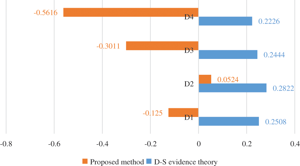
Figure 3: The comparison of the assessment results of proposed method and D-S evidence theory

According to the nature of correlation function, the assessment result is analyzed as follows. The grade of each indicator, which is shown in Fig. 4, can reflect the main problems existing in power grid.

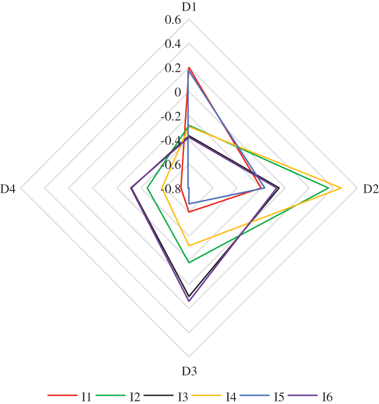
Figure 4: The grade of each indicator

As can be seen in Table 12, the grade of frequency deviation (I1) is D1, the grade of total harmonic distortion rate of voltage (I2) is D2, the grade of voltage fluctuation (I3) is D3, the grade of voltage flicker (I4) is D2, the grade of voltage deviation (I5) is D1 and the grade of voltage three-phase unbalance degree (I6) is D3. Compared with other indicators, voltage fluctuation (I3) and voltage three-phase unbalance degree (I6) have lower assessment grade. Therefore, voltage fluctuation and voltage three-phase unbalance degree are the key factors affecting power quality, and corresponding measures should be taken to restrain these two indicators.

5  Conclusions

In this paper, the method of combining extension analysis with rough AHP is used to assess power quality comprehensively. By rough AHP, the adverse effects of single expert judgment can be eliminated. Through the concept of matter-element and correlation function, the relationship between each assessment indicator of power quality and the assessment interval of each quality grade can be quantified. At last the case analysis and application show that the proposed method can determine the overall power quality of power grid, compare the differences among the performance of assessment indicators, find out the key factors affecting power quality, and provide the basis for further improving the power quality of power grid. However, rough AHP is a kind of subjective weighting method and may lead to the lack of effective weighting information. Synthesis of subjective and objective weights is a significant way to overcome this shortcoming. In addition, the definition of assessment grade standard, classical domain and joint domain needs to be further studied in extension analysis.

Funding Statement: The authors received no specific funding for this study.

Conflicts of Interest: The authors declare that they have no conflicts of interest to report regarding the present study.

This work is licensed under a Creative Commons Attribution 4.0 International License, which permits unrestricted use, distribution, and reproduction in any medium, provided the original work is properly cited.