| Energy Engineering |
DOI: 10.32604/ee.2022.019072
ARTICLE
Two Phase Flow Simulation of Fractal Oil Reservoir Based on Meshless Method
1School of Petroleum Engineering, Yangtze University, Wuhan, 430100, China
2China Oilfield Services Limited, Tianjin, China
3Xinmin Oil Production Plant of Jilin Oilfield Company, PetroChina, Songyuan, 138000, China
*Corresponding Author: Yunfeng Xu. Email: 201972114@yangtzeu.edu.cn
Received: 01 September 2021; Accepted: 21 October 2021
Abstract: The reservoir is the networked rock skeleton of an oil and gas trap, as well as the generic term for the fluid contained within pore fractures and karst caves. Heterogeneity and a complex internal pore structure characterize the reservoir rock. By introducing the fractal permeability formula, this paper establishes a fractal mathematical model of oil-water two-phase flow in an oil reservoir with heterogeneity characteristics and numerically solves the mathematical model using the weighted least squares meshless method. Additionally, the method's correctness is verified by comparison to the exact solution. The numerical results demonstrate that the fractal oil-water two-phase flow mathematical model developed using the meshless method is capable of more accurately and efficiently describing the flow characteristics of the oil-water two-phase migration process. In comparison to the conventional numerical model, this method achieves a greater degree of convergence and stability. This paper examines the effect of varying the initial viscosity of the oil, the initial formation pressure, and the production and injection ratios on daily oil production per well, water cut in the block, and accumulated oil in the block. For 10 and 60 cp initial crude oil viscosities, the water cut can be 0.62 and 0.80, with 3100 and 1900 m3 cumulative oil production. Initial pressures have little effect on production. In this case, the daily oil production of well PRO1 is 1.7 m3 at 7 and 10 MPa initial pressure. Block cumulative oil production is 3465.4 and 2149.9 m3 when the production injection ratio is 1.4 and 0.8. The two-phase meshless method described in this paper is essential for a rational and effective study of production dynamics patterns in complex reservoirs and the development of reservoir simulations of oil-water flow in heterogeneous reservoirs.
Keywords: Oil-water two-phase flow; fractal theory; weighted least square method; meshless method
Nomenclature
| Density of oil and water respectively (kg/m3); | |
| Fractal permeability (mD); | |
| Relative permeability of water phase and oil phase (mD); | |
| Viscosity of oil phase and water phase mPa⋅s; | |
| Pressure of oil phase and water phase in Reservoir (MPa); | |
| Fractal porosity; | |
| Saturation of water phase and oil phase; | |
| t | production time (day); |
| Source-sink phase under standard conditions (m3/day). |
The reservoir is the network of rock skeletons that surround a sealed oil and gas trap, as well as the generic term for the fluid contained in pore fractures and karst caves. The heterogeneity and complexity of reservoir rock have a significant effect on reservoir physical properties such as flowability, reservoir capacity, and rock particle adsorption capacity. To maximize recovery, it is necessary to master the situation of underground reservoirs as much as possible during oil field development [1]. However, because the reservoir's porous media are largely disordered, it is impossible to accurately describe the reservoir's actual characteristics when the reservoir is approximated as a homogeneous model. The introduction of fractal theory enables us to better understand the pore results and transport properties of porous media [2]. Thus, over the last two decades, extensive research on the transport characteristics of porous media in oil reservoirs based on fractal theory has been conducted in the field of petroleum engineering [3].
Mandelbrot pioneered the concept of a fractal, which is used to describe the geometry found in nature that is self-similar and has no feature length [4]. In 1985, Katz et al. [5] demonstrated that sandstone interstitial space and pore surface exhibit favorable fractal characteristics through a large number of data analyses. The relationship between fractal dimension and rock porosity can be determined using the derived formula, and the porosity value can be calculated using a logarithmic curve [5]. Chang et al. pioneered the application of fractal theory to porous media mechanics, proposing the use of fractal dimension and fractal index to describe the complexity of porous media pore structure, and establishing the fractal Flow model of reservoir, which is used to reflect the reservoir's dynamic characteristics [6].
The majority of the research on fractal reservoirs discussed above makes use of numerical models based on grid systems, such as the finite difference method (FDM) and the finite element method (FEM) [7]. To provide an accurate description of the morphology and laws governing heterogeneous reservoirs, A large number of grids must be divided in the grid system, and the processing before and after is time-consuming, as is the calculation. This paper employs a meshless numerical model to create a stable, reliable, and accurate numerical model [8]. This method is a meshless version of the weighted least squares method (MWLS) [9]. In comparison to the finite difference and finite element methods, this method has the advantages of avoiding grid generation, requiring minimal data preparation, and allowing for convenient handling both before and after. The first meshless method was proposed by Lucy [10] in 1977 and successfully applied to astrophysical problems. Later that year, in 1996, Spanish researchers E Onate proposed the finite point method (FPM) [11]. This method constructs the shape function using the moving least squares principle and discretizes it using the collocation scheme; it is a completely meshless method that does not require a background grid and is primarily used in the field of fluid mechanics. Atluri et al. [12] and colleagues proposed the Meshless Local Galerkin method in 1998, which eliminated the need for a background grid when integrating. For the first time, Yousef et al. [13] applied the MWLS method to a complex fault block hydrocarbon reservoir numerical good test and obtained satisfactory results in terms of calculation accuracy and efficiency. Xu et al. [14] used fractal theory to characterize the permeability and porosity of horizontal shale gas fracturing wells, although they solved the gas-water two-phase flow model using the weighted least squares meshless method [15].
This Paper introduces the fractal permeability expression, establishes a numerical model of fractal oil reservoir two-phase, and solves it using the weighted least squares meshless method (MWLS). Relevant examples are provided to demonstrate the accuracy and benefits of this method.
(1) Assume that the outer boundary of the reservoir is closed; (2) Fluid and rock micro-compressibility; (3) Isothermal flow event, ignoring heat dissipation; (4) The model applies to oil-water two-phase, and the two are not mixed; (5) Ignore the influence of capillary force.
The distribution of reservoir porosity and permeability conforms to the following rules:
In the formula,
2.2 Weighted Least-Squares Meshless Method
The meshless method can be theoretically justified using the weighted residual method. The Moving Least Square method (SLS) is used to construct approximate functions in this paper, followed by the Least Square method to discretize the governing equations and establish the corresponding meshless method, namely the weighted least squares meshless method (MWLS). For more information about the weighted least squares meshless method, see reference [14].
The time items of the above Eqs. (1) and (2) can be sorted out by difference. The following Eq. (5) can be obtained
Among them,
The above Eq. (5) obtains residual Eqs. (6) and (7):
In Eqs. (6) and (7), the sum refers to the residual quantity of pressure equation and water saturation equation.
For residual changes:
The MWLS form of the oil phase pressure equation can be obtained as follows:
Considering
which:
Water saturation MWLS is calculated as follows:
Considering
which:
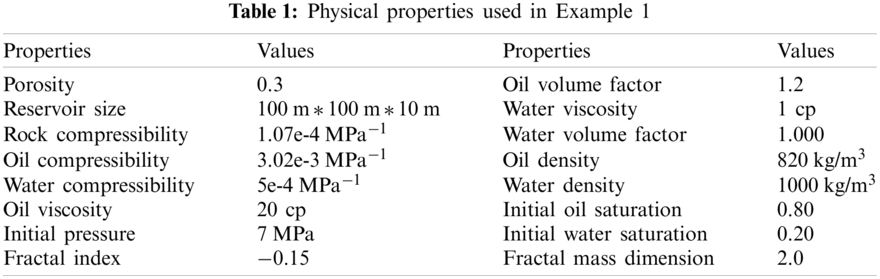
Based on the theoretical research described above, a two-dimensional oil-water two-phase numerical simulation model with fractal properties is established. The model is 100 m ∗ 100 m ∗ 10 m in size, with the injection well IN1 in the center, the production wells distributed around it, an injection rate of 20 m3/day, a recovery rate of 5 m3/day, and a production time of 200 days. The model's permeability distribution is depicted in Fig. 1. The model's heterogeneous characteristics are readily apparent. The distribution interval for this paper is 5 m, and Table 1 contains some physical property information. The weighted least squares meshless method is used in this paper, and the node influence domain is set to three.

Figure 1: Permeability field diagram
The Buckley-Leverett [16] method is used to verify the accuracy of this method. As illustrated in Fig. 2, the accuracy of this method is nearly identical to that of Bekele, with an error of less than 2%; thus, the accuracy of this method can be seen. Additionally, the method described in this paper does not require grid division, and its convergence and stability are significantly higher than those of traditional numerical simulation methods. Additionally, as illustrated in Fig. 3, the daily oil production of well PRO1 decreases significantly less than that of well PRO3. As can be seen, the characteristics of heterogeneous reservoirs are quite apparent.

Figure 2: Comparison of the oil production rate of a single well (a) #PRO1 (b) #PRO2 (c) #PRO3 (d) #PRO4

Figure 3: Comparison of the oil production rate of #PRO1 and #PRO3
Sensitivity analysis is performed on the initial crude oil viscosity, initial water saturation, initial pressure, and other parameters that affect the production dynamic data, and then the correctness of this method is verified in the numerical solution of fractal reservoir oil-water two-phase flow using the above-mentioned theories and methods.
4.1 Effect of Initial Crude Oil Viscosity
The initial formation pressure is the critical factor affecting the reservoir's daily oil production. The development benefit of the reservoir can be determined using the initial formation pressure, which more intuitively reflects the reservoir's crude oil diversion capacity. In this paper, the initial formation pressures of 7, 8, 9, and 10 MPa are used for simulation to ensure that the other physical parameters are consistent with Table 1. The weighted least squares meshless method makes use of a Gaussian basis function and a three-dimensional node influence domain. The fractal index is −0.15 and the fractal mass dimension is 2.0.
Fig. 4 illustrates the daily oil production of each well for various initial crude oil viscosities. As shown in Fig. 4, after 200 days, the initial crude oil viscosity is 10 cp, and the well PRO1 produces 2.35 m3/day of oil. When the initial viscosity of the crude oil is 60 cp, however, well PRO1 produces only 1.23 m3/day of oil. The higher the initial crude oil viscosity, the shorter the time required for water to penetrate the reservoir. As illustrated in Fig. 5, the initial crude oil viscosity influences the rate at which the block moisture content increases. When the initial crude oil viscosity is ten times that of water, the block moisture content in 200 days is only 0.62, but when the initial crude oil viscosity is sixty times that of water, the block water cut can reach 0.80. This is primarily because the initial crude oil viscosity is higher, the crude oil mobility is lower, and the reservoir's water flow capacity is greater. As shown in Fig. 6, after 200 days, the initial crude oil viscosity is 10 cp, and the block's accumulated oil can reach 3100 m3. However, the block's cumulative oil production is limited to 1900 m3 due to the initial crude oil viscosity of 60 cp. The lower the initial viscosity, the greater the accumulation of oil in the block, which is primarily determined by the two-phase flow mobility ratio.
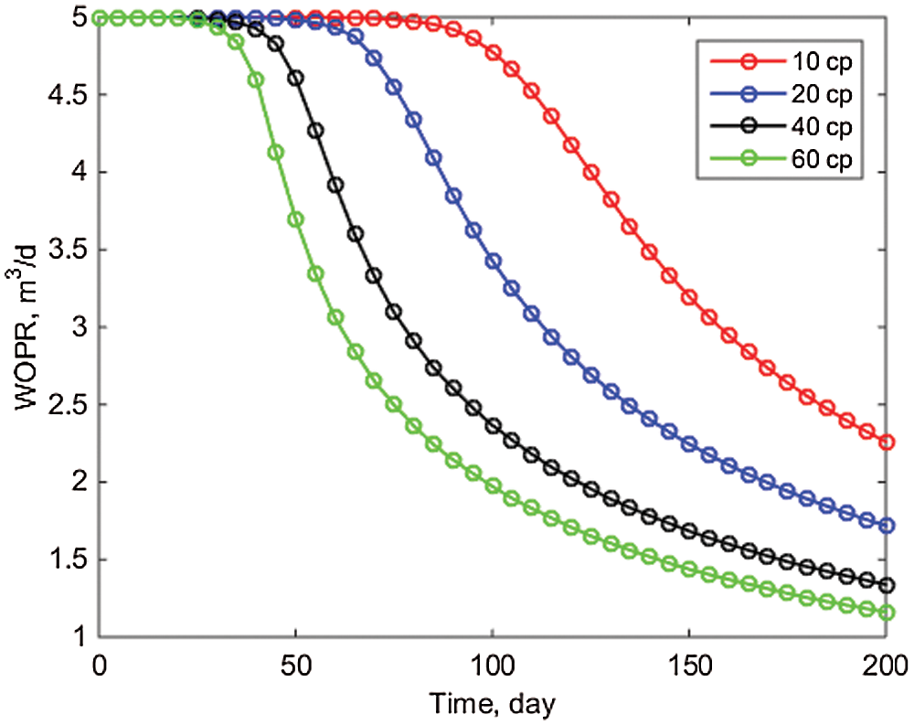
Figure 4: Comparison of daily oil production of well POR1
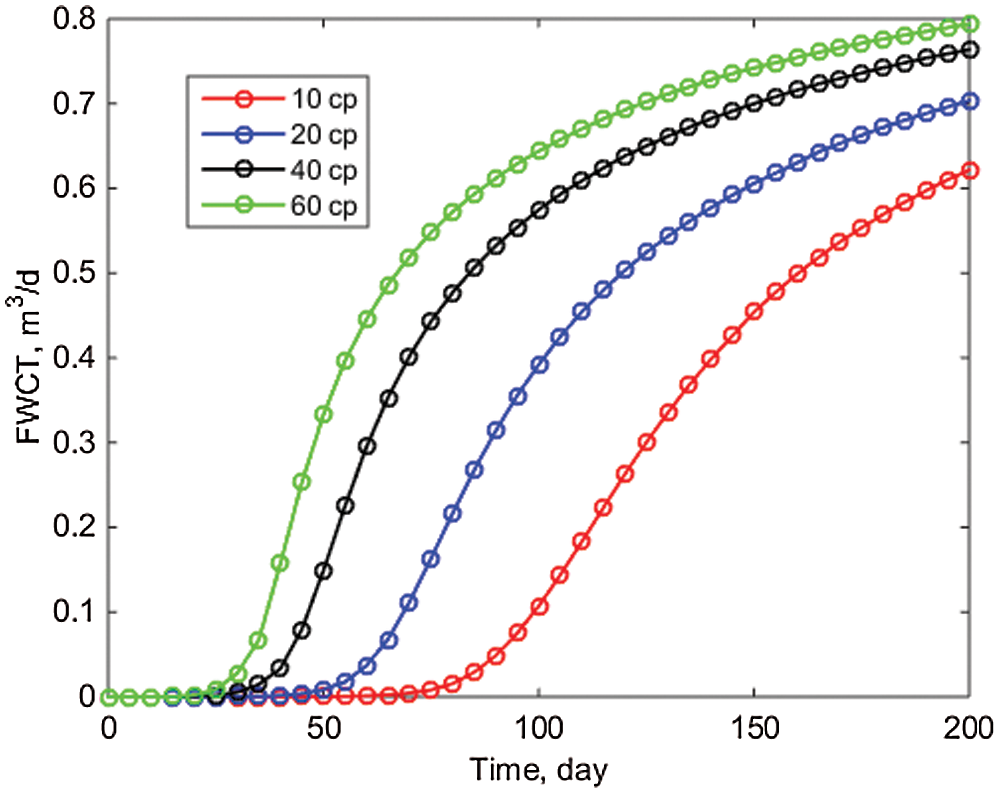
Figure 5: Block water cut
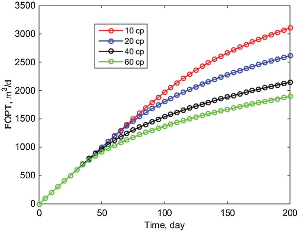
Figure 6: Oil production in block
4.2 Influence of Initial Formation Pressure
The initial formation pressure is the critical factor affecting the reservoir's daily oil production. The development benefit of the reservoir can be determined using the initial formation pressure, which more intuitively reflects the reservoir's crude oil diversion capacity. In this paper, the initial formation pressures of 7, 8, 9, and 10 MPa are used for simulation to ensure that the other physical parameters are consistent with Table 1. The weighted least squares meshless method makes use of a Gaussian basis function and a three-dimensional node influence domain. The fractal index is −0.15 and the fractal mass dimension is 2.0.
The pressure change value for well PRO1 at various initial formation pressures is depicted in Fig. 7. As illustrated in Fig. 7, when the initial formation pressure changes over time, the decrease range is not large, owing to the small amount of produced fluid used in this paper and the small pressure drop required at the wellhead. As illustrated in Fig. 8, when the initial formation pressure changes, the daily oil production per well essentially does not match. This is because, while crude oil production is determined by the pressure difference, in this paper, different initial formation pressure cannot affect daily oil production under the assumption of fixed liquid production.
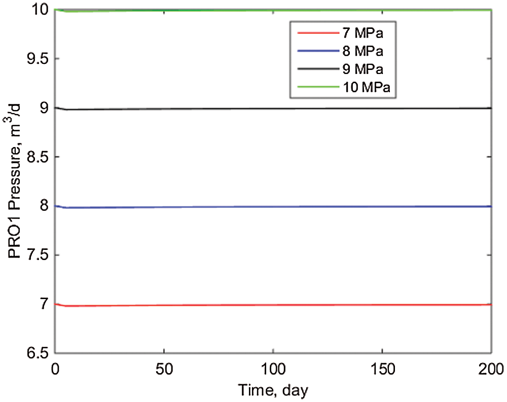
Figure 7: Pressure value of well PRO1
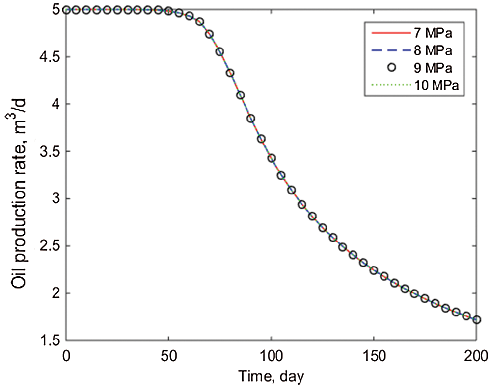
Figure 8: Comparison of daily oil production of well PRO1
4.3 Effect of Injection and Production Parameters
In actual reservoir production, injection-production parameters are critical for maximizing economic benefits. The injection volume is kept constant in this paper, and simulations using the production-injection ratios of 0.8, 1.0, 1.2, and 1.4 are used to ensure that all other physical parameters are consistent with Table 1. The weighted least squares meshless method makes use of a Gaussian basis function and a three-dimensional node influence domain. The fractal index is −0.15, and the fractal mass dimension is 2.0.
From Figs. 9–11, it is clear that the block's water cut and accumulated oil increase as the production and injection ratios increase. When the production-injection ratio is 1.4, the FWCT after 300 days can reach 0.7322 and the FOPT can reach 3465.4 m3, but when the injection ratio is 0.8, the FWCT after 300 days is only 0.6872 and the FOPT is only 2149.9 m3, while when the injection ratio is 0.8, the FWCT after 300 days is only 0.6872 and the FOPT is only 2149.9 m3. Therefore, if the water cost of processing production is low, increasing the injection ratio can result in a higher FOPT, which can be used to guide production.
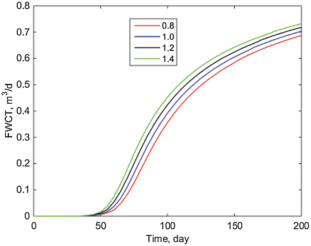
Figure 9: Block water cut
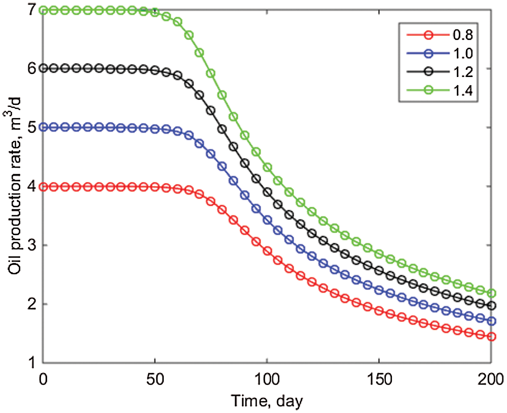
Figure 10: Comparison of daily oil production of well POR1
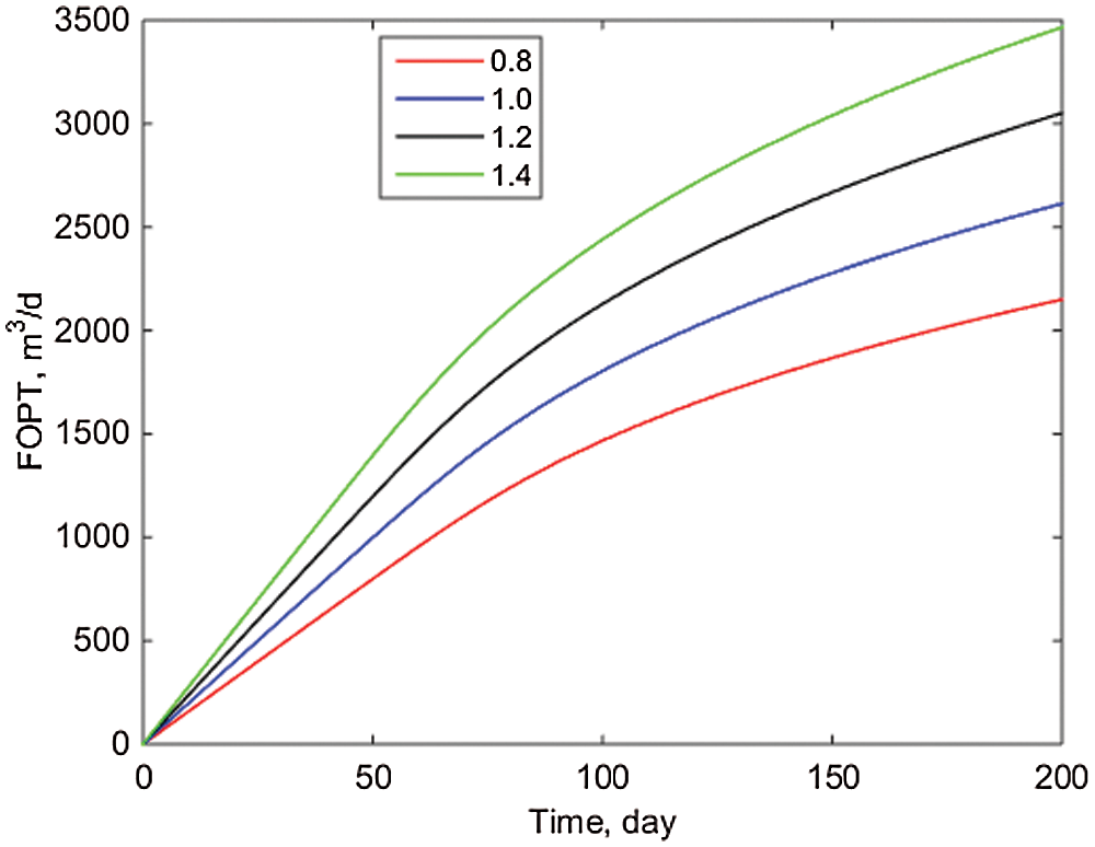
Figure 11: Oil production in block
The weighted least squares meshless method is introduced in this paper to solve an oil reservoir oil-water two-phase flow model with fractal characteristics. The fractal permeability formula is used to establish a fractal mathematical model of oil-water two-phase flow in an oil reservoir that takes heterogeneity into account, and the mathematical model is numerically solved using the weighted least squares meshless method. The following are the major conclusions:
(1) According to the model developed in this paper, the difference between this method and the analytical model is only 2%. The numerical results demonstrate that using the meshless method, the fractal oil-water two-phase flow mathematical model can more accurately and efficiently describe the flow characteristics of the oil-water two-phase migration process.
(2) The effects of varying the initial crude oil viscosity on the daily oil production of a single well, water cut, and cumulative oil production are examined in this article. When the initial crude oil viscosity is 10 and 60 cp, the water cut can reach 0.62 and 0.80, respectively, resulting in cumulative oil production of 3100 and 1900 m3. According to objective facts, this method's stability and convergence are also demonstrated from the side.
(3) This paper investigates the effect of different initial formation pressures on the daily output of a single well and the pressure of a single well, concluding that different initial formation pressures do not affect the output. This is consistent with the objective understanding that differential pressure drives oil-water two-phase flow in reservoir production. In this example, the daily oil production of well PRO1 is 1.7 m3 in 200 days when the initial pressure is 7 and 10 MPa.
(4) This paper relates the effects of various production injection ratios on daily oil production from a single well, block water cut, and cumulative oil production from a block. When the production injection ratio is 1.4 and 0.8, respectively, the block water cut is 0.7322 and 0.6872, and the cumulative oil production of the block is 3465.4 and 2149.9 m3, respectively. As a result, during actual production, the injection ratio should be rationally planned to maximize economic benefit.
Funding Statement: The National Natural Science Foundation of China (Nos. 51874044, 51922007).
Conflicts of Interest: The authors declare that they have no conflicts of interest to report regarding the present study.
1. Freeze, R. A. (1980). A stochastic-conceptual analysis of rainfall-runoff processes on a hillslope. Water Resources Research, 16(2), 391–408. DOI 10.1029/WR016i002p00391. [Google Scholar] [CrossRef]
2. Rao, X., Zhan, W., Zhao, H., Xu, Y., Liu, D. et al. (2021). Application of the least-square meshless method to gas-water flow simulation of complex-shape shale gas reservoirs. Engineering Analysis with Boundary Elements, 129, 39–54. DOI 10.1016/j.enganabound.2021.04.018. [Google Scholar] [CrossRef]
3. Miao, T., Yu, B., Duan, Y., Fang, Q. (2015). A fractal analysis of permeability for fractured rocks. International Journal of Heat Mass Transfer, 81, 75–80. DOI 10.1016/j.ijheatmasstransfer.2014.10.010. [Google Scholar] [CrossRef]
4. Mandelbrot, B. B. (1983). The fractal geometry of nature. American Journal of Physics, 51(3), 286–286. DOI 10.1119/1.13295. [Google Scholar] [CrossRef]
5. Katz, A. J., Thompson, A. H. (1985). Fractal sandstone pores: Implications for conductivity and pore formation. Physical Review Letters, 54(12), 1325–1328. DOI 10.1103/PhysRevLett.54.1325. [Google Scholar] [CrossRef]
6. Chang, J., Yortsos, Y. C. (1990). Pressure transient analysis of fractal reservoirs. SPE Formation Evaluation, 5(1), 31–38. DOI 10.2118/18170-PA. [Google Scholar] [CrossRef]
7. Rao, X. (2018). A novel green element method based on two sets of nodes. Engineering Analysis with Boundary Elements, 91, 124–131. DOI 10.1016/j.enganabound.2018.03.017. [Google Scholar] [CrossRef]
8. Xiong, Z., Yan, L. (2004). Meshless methods. China: Tsinghua Publishing House. [Google Scholar]
9. Zhao, H., Xu, L., Guo, Z., Zhang, Q., Liu, W. et al. (2019). Flow-path tracking strategy in a data-driven interwell numerical simulation model for waterflooding history matching and performance prediction with infill wells. SPE Journal, 25(2), 1007–1025. DOI 10.2118/199361-PA. [Google Scholar] [CrossRef]
10. Lucy, L. B. (1993). Numerical approach to testing of fission hypothesis. The Astronomical Journal, 82, 1013–1024. DOI 10.1086/112164. [Google Scholar] [CrossRef]
11. Oñate E, I. S. (1996). A finite point method in computational mechanics applications to convective transport and fluid flow. International Journal for Numerical Methods in Engineering, 39(22), 3839–3866. DOI 10.1002/(ISSN)1097-0207. [Google Scholar] [CrossRef]
12. Atluri, S. N., Zhu, T. (1998). A new meshless local petrov-galerkin (MLPG) approach in computational mechanics. Computational Mechanics, 22(2), 117–127. DOI 10.1007/s004660050346. [Google Scholar] [CrossRef]
13. Yousef, A. A., Gentil, P. H., Jensen, J. L., Lake, L. W. (2006). A capacitance model to infer interwell connectivity from production and injection rate fluctuations. SPE Reservoir Evaluation Engineering, 9(6), 630–646. DOI 10.2118/95322-PA. [Google Scholar] [CrossRef]
14. Xu, Y., Sheng, G., Zhao, H., Hui, Y., Zhou, Y. et al. (2021). A new approach for gas-water flow simulation in multi-fractured horizontal wells of shale gas reservoirs. Journal of Petroleum Science Engineering, 199, 108292. DOI 10.1016/j.petrol.2020.108292. [Google Scholar] [CrossRef]
15. Zhao, H., Sheng, G. L., Huang, L. Y., Zhong, X. (2021). Application of lightning breakdown simulation in inversion of induced fracture network morphology in stimulated reservoirs. International Petroleum Technology Conference. [Google Scholar]
16. Spayd, K., Shearer, M. (2011). The buckley-leverett equation with dynamic capillary pressure. SIAM Journal on Applied Mathematics, 71(4), 1088–1108. DOI 10.1137/100807016. [Google Scholar] [CrossRef]
 | This work is licensed under a Creative Commons Attribution 4.0 International License, which permits unrestricted use, distribution, and reproduction in any medium, provided the original work is properly cited. |