Energy Engineering

DOI: 10.32604/EE.2021.015145

ARTICLE

A Weighted Combination Forecasting Model for Power Load Based on Forecasting Model Selection and Fuzzy Scale Joint Evaluation

Bingbing Chen*, Zhengyi Zhu, Xuyan Wang and Can Zhang

State Grid Nanjing Power Supply Company, Nanjing, 210019, China
*Corresponding Author: Bingbing Chen. Email: flying387@aliyun.com
Received: 25 November 2020; Accepted: 21 December 2020

1  Introduction

Medium and long term power load forecasting is the main basis of power special planning and distribution network planning. Its forecasting accuracy is directly related to the quality of planning scheme, and is also defined as an important index to evaluate the modernization degree of power enterprise management. In addition, medium and long term load forecasting plays an important role in the security and economy of power grid. Therefore, it has become an urgent problem to study the forecasting method and improve the load forecasting accuracy in the development of power system. However, in recent years, the power market demand has changed greatly, from the initial shortage of supply and demand to the current overall balance of supply and demand. Some new characteristics emerge from the change of power load, which brings a lot of complex factors to the forecasting work.

The single load forecasting model is restricted by the fixed scope of application, so it is difficult to be used in all cases. Selecting multiple models to combine can not only make up the limitation of the information of a single model, but also bring good properties to different models. Compared with single forecasting model, the forecasting results of various models are more effective and comprehensive [1,2]. The research focus of combination forecasting is combination model selection and combination weight determination. The existing model selection [3,4] uses analog error to determine the analog accuracy based on the error of forecasting results, and uses analog error to replace or approximate the forecasting accuracy based on the principle of continuity, so as to carry out model selection. However, there is a lack of recognition of the transfer law from analog accuracy to forecasting accuracy. The combination methods include constant weight and variable weight. Variable weight combination has good adaptability, but it is difficult to reflect the forecasting effectiveness of the model based on error theory.

At present, the commonly used combination methods include minimum variance method, variance covariance method, optimal combination method and analytic hierarchy process [5–7]. Niu et al. [8] and Xiao et al. [9] used Bayesian theory and structural risk minimization principle to establish the least squares support vector machine (LSSVM) combined forecasting model for power load. Ma et al. [10] proposed that the optimal combination forecasting technology can be divided into two parts: Model screening and combination screening. Jiang et al. [11] further analyze the advantages and disadvantages of the screening method, use grey correlation degree method to improve and establish variable weight combination forecasting model. Zhou et al. [12] used entropy method, variance covariance method and grey method to construct hierarchical structure to determine the weight of each model. To eliminate the redundant information in the prediction method, You et al. [13] tested each prediction model for redundancy one by one in combination, regarded the weight as a fuzzy number, and then obtained the optimal weight coefficient through the properties of fuzzy number.

Markov chain is a stochastic process with Markov property in probability theory and mathematical statistics and exists in discrete index set and state space, which is widely used in boundary estimation. Wilinski [14] studied the prediction in a financial time series based on a model in the form of Markov chains. Arruda et al. [15] focused on the computation of the steady state distribution of a Markov chain and made use of an embedding algorithm. Zhu et al. [16] put forward a wind power time series modeling method based on the improved Markov Chain Monte Carlo method. Wan et al. [17] optimized the foundation pit settlement prediction model of logistic curve based on Markov chain. Cloud algorithm is also a powerful tool for load forecasting. Wang et al. [18] proposed a new model with combination of cloud model and support vector machine to select the parameters of the kernel function more accurately and improve the accuracy of short-term load forecasting. Wei et al. [19] introduced a new method and theory of power emergency group decision-making based on cloud model for the power emergency evaluation system established by analytical hierarchy process (AHP). Wang et al. [20] proposed a new model which is combined by the cloud model, particle swarm optimization (PSO) and LSSVM to improve the accuracy of selecting the parameters of the kernel function, to deal with uncertainty factors and improve the accuracy of short-term load forecasting. Liu et al. [21] proposed a method based on cloud model and fuzzy Petri net to solve the problem that it is difficult to identify and control the potential hazardous trading behavior in the power market.

In order to further expand the combination forecasting method, based on previous studies, this paper applies the idea of Markov chain conversion and cloud algorithm to forecasting model selection and proposed a weighted combination forecasting model for medium and long-term power load forecasting. By forecasting the power consumption of the whole society in a certain area, the forecasting results show the effectiveness of the proposed model, and its practical value is well verified.

2  Research Structure

This paper expands the combination forecasting method for the medium and long term power load forecasting problem and proposes a weighted combination forecasting model. The flowchart of the proposed model is shown in Fig. 1.

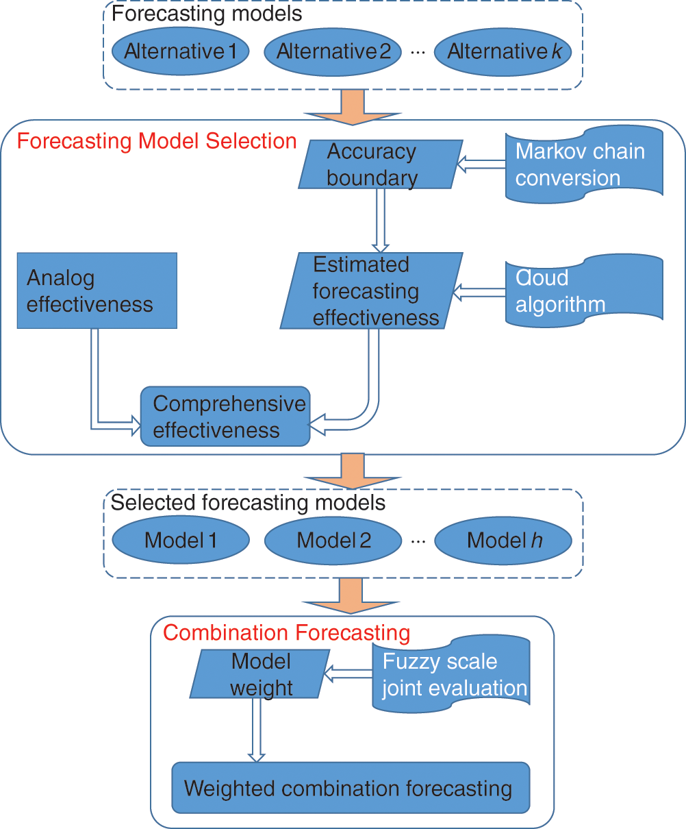
Figure 1: The flowchart of the proposed weighted combination forecasting model

As shown in Fig. 1, the proposed model is divided into two stages: Forecasting model selection and combination forecasting. In the first stage, the forecasting accuracy boundary of forecasting model is determined by Markov chain conversion, and then the estimated forecasting effectiveness is determined by cloud algorithm. After this, the comprehensive effectiveness of forecasting model can be obtained by integrating the analog effectiveness and estimated forecasting effectiveness. According to the comprehensive effectiveness of forecasting model several outstanding models are selected for the combination forecasting. In the second stage, fuzzy scale joint evaluation is carried out to determine the weight of selected forecasting model. Based on the model weight and single model forecasting value, weighted combination forecasting is implemented.

3  Forecasting Model Selection

It is assumed that there are m history years and the power load of history year i is ρi , here i = 1, 2, …, m. There are n forecasting years and the forecasting power load of forecasting year j is ϑj , here j = 1, 2…n. There are k alternatives of forecasting models. Through forecasting model l, the analog value of power load of history year i is ρl,i′ while the forecasting value of power load of forecasting year j is ϑl,j′ , here l = 1, 2…k.

For forecasting model l, the analog value relative error ηl,i of history year i and forecasting value relative error ηl,j of forecasting year j are:

ηl,i=(ρi−ρ′l,i)/(ρi−ρ′l,i)ρiρi (1)

ηl,j=(ϑj−ϑ′l,j)/(ϑj−ϑ′l,j)ϑjϑj (2)

If 0≤|ηl,i|≤1 , the analog accuracy of history year i is θl,i=1−|ηl,i| ; If |ηl,i|>1 , the analog accuracy of history year i is θl,i=0 . Similarly, if 0≤|ηl,j|≤1 , the forecasting accuracy of forecasting year j is θl,j=1−|ηl,j| ; If |ηl,j|>1 , the forecasting accuracy of history year i is θl,j=0 .

Next the analog effectiveness μl and forecasting effectiveness νl of forecasting model l are:

μl=∑i=1mθl,im(1−σ(θl,i)) (3)

νl=∑j=1nθl,in(1−σ(θl,j)) (4)

Here σ(θl,i) is the standard deviation of θl,i and σ(θl,j) is the standard deviation of θl,j .

The comprehensive effectiveness of forecasting model l is defined by Eqs. (3) and (4), which characterizes the credibility of the forecasting model. In the future forecasting interval, the practical power load value has not yet appeared and the forecasting value relative error (Eq. (2)) cannot be obtained. The accuracy and the effectiveness of a forecasting model can only be estimated based on its inherent property. After that, the forecasting models are screened and the better forecasting models are selected to implement combination forecasting.

The accuracy of forecasting model is an inherent property. The analog accuracy, which can be obtained by the virtual forecasting for the multi-time power load, is a performance of the accuracy of forecasting model. Through forecasting model l the power load of history year i is forecasted. Then the analog accuracy sequence is obtained as {θl,1,θl,2,...,θl,m} . In {θl,1,θl,2,...,θl,m} , the expectation and the standard deviation of the analog accuracy of each history year show the property of the forecasting model. As everyone knows, randomness and discreteness always appear in analog accuracy sequence {θl,1,θl,2,...,θl,m} . In view of this, Markov chain conversion matrix [22] can be adopted to describe the conversion principle. The accuracy boundary is estimated based on Markov chain by the following steps.

Step 1: For forecasting model l the distribution interval of analog accuracy of history year i can be equally divided into ml subintervals which are ϖl,1,ϖl,2,...,ϖl,ml , here ml≤m . Each subinterval can be treated as an analog accuracy status. All analog accuracy statuses form a status sequence {ϖl,1,ϖl,2,...,ϖl,ml} .

Step 2: Based on the analog accuracy of forecasting model l of history year i, it is assumed that the appearance number of analog accuracy status ϖl,s is ANl,s , here s=1,2,...,ml and ANl,s<m . It means that there are ANl,s times belonging to analog accuracy status ϖl,s . Assuming that the conversion times from status ϖl,g to status ϖl,s is Cl(g,s) . Therefore, the conversion probability of forecasting model l from status ϖl,g to status ϖl,s is obtained as:

Pl(g,s)=Cl(g,s)ANl,s (5)

Step 3: The 1st order status conversion matrix of forecasting model l is constructed as:

Pl(1)=[Pl(g,s)]m′×m′ (6)

Then the qth order status conversion matrix of forecasting model l is obtained as:

Pl(q)=(Pl(1))q (7)

Step 4: For forecasting model l, the appearance numbers of every analog accuracy status form an initial vector ANl as:

ANl=[ANl,1,ANl,2,...,ANl,ml] (8)

A new status matrix of forecasting model l can be obtained by multiplying initial vector ANl and qth order status conversion matrix Pl(q) :

Pl=ANl⋅Pl(q) (9)

Step 5: The sum of every column of Pl is calculated one by one. Assuming that the column with the maximum sum is column s, the forecasting accuracy belongs to accuracy status ϖl,s . Therefore, the accuracy boundary estimation of forecasting model l is obtained.

In m history years, affected by various kinds of factors, analog accuracy sequence {θl,1,θl,2,...,θl,m} of forecasting model l obviously has the features of random variables. Therefore, the forecasting accuracy is equivocal in the accuracy boundary (obtained in Step 5). The non-determinacy in the accuracy boundary can be described by the concepts of expectation, entropy and hyper-entropy in cloud model theory [23]. Then the accuracy can be estimated quantitatively by the following steps.

Step 6: Based on reverse cloud algorithm, analog accuracy sequence {θl,1,θl,2,...,θl,m} is treated as the input of cloud model while expectation αl , entropy βl and hyper-entropy γl is the output of cloud model. The reverse cloud algorithm is:

(1) Expectation:

αl=∑i=1mθl,im (10)

(2) 1st order absolute center distance:

Ω1=1m∑i=1m|θl,i−αl| (11)

(3) 2nd order absolute center distance:

Ω2=1m−1∑i=1m(θl,i−αl)2 (12)

(4) Entropy:

βl=π2Ω1 (13)

(5) Hyper-entropy:

γl=Ω2−(βl)2 (14)

Step 7: By treating expectation αl , entropy βl and hyper-entropy γl as the input of forward cloud generator and treating accuracy boundary ϖl,s as constraint, the accuracy is estimated quantitatively by forward cloud model. The forward cloud algorithm is:

(1) A normal random number is generated with an expectation of βl and a variance of γl :

Ψ=NORM(βl,γl) (15)

(2) In accuracy boundary ϖl,s , normal random forecasting accuracy is generated with an expectation of αl and a variance of Ψ :

θl,j=NORM(αl,Ψ) (16)

Next forecasting model selection is carried out based on the comprehensive effectiveness of each forecasting model. In m history years and n forecasting years, the comprehensive effectiveness of forecasting model l is defined based on Eqs. (3) and (4) as:

εl=λ⋅μl+η⋅νl (17)

Here, μl is the analog effectiveness of forecasting model l in m history years and νl is the estimated forecasting effectiveness of forecasting model l in n forecasting years. λ and η are the importance factors of analog effectiveness and forecasting effectiveness respectively which satisfy:

{λ+η=1λ>0,η>0 (18)

The threshold value of forecasting model selection is determined by:

ε¯=∑l=1kεlk (19)

When εl is greater than or equal to threshold value ε¯ , forecasting model l is selected for the subsequent combination forecasting.

4  Combination Forecasting

It is assumed that there are h selected forecasting models, here h < k. How to determine the weight of each model is a key problem in combination forecasting. In the weight determination problem, expert evaluation method can make full use of the experience and wisdom of experts. In this paper, the expert evaluation method is introduced into the determination of forecasting model weight. Experts make a judgment on the principle of the model, the degree of agreement with the actual situation and the forecasting effect, so as to determine the weight of the model. In the traditional expert evaluation method, the accurate scale value is used to express the experts’ evaluation on the importance of different objects [24]. Compared with the accurate scale value, the fuzzy scale value can better reflect the uncertainty of expert evaluation. In addition, compared with the single expert evaluation, the joint evaluation of multiple experts is more reasonable. Therefore, this paper proposes a fuzzy scale joint evaluation method to determine the weight of forecasting model. In proposed method, trapezoid fuzzy number is used to express the experts’ evaluation on the importance of different forecasting models and rough boundary interval is used to integrate the judgments of different experts. Its detailed process is as following.

Step 1: It is assumed that there are t experts. For h selected forecasting models, each expert evaluates the relative importance of any two selected forecasting models. The fuzzy reciprocal evaluation matrix given by expert r (r = 1, 2, …, t) is as:

E~r=[e~x,yr]h×h (20)

Here e~x,yr is the evaluation score of model x relative to model y given by expert r. e~x,yr is a trapezoid fuzzy number scale and e~x,yr=(ξx,yr,ςx,yr,ψx,yr,ζx,yr) . If x = y, e~x,yr = (1,1,1,1). The next step can only be carried out after t evaluation matrices are qualified in consistency inspection. Otherwise, the corresponding expert will adjust his evaluation matrix.

Step 2: The joint evaluation matrix is constructed as:

E~=[e~x,y]h×h (21)

Here e~x,y={e~x,y1,e~x,y2,...,e~x,yt} .

Step 3: According to rough sets theory [25,26], the rough boundary interval of e~x,yr in e~x,y can be expressed as:

RBI(e~x,yr)=[L_(e~x,yr),L¯(e~x,yr)] (22)

L_(e~x,yr)=∑e~x,yr_≤e~x,yre~x,yr_N_(e~x,yr) (23)

L¯(e~x,yr)=∑e~x,yr¯≥e~x,yre~x,yr¯N¯(e~x,yr) (24)

Here L_(e~x,yr) is the rough lower boundary of RBI(e~x,yr) and L¯(e~x,yr) is the rough upper boundary of RBI(e~x,yr) , N_(e~x,yr) means the number of the elements which smaller than or equal to e~x,yr and N¯(e~x,yr) means the number of the elements which bigger than or equal to e~x,yr .

Then the rough boundary interval of e~x,y can be expressed as:

RBI(e~x,y)=[L_(e~x,y),L¯(e~x,y)] (25)

L_(e~x,y)=∑r=1tL_(e~x,yr)t (26)

L¯(e~x,y)=∑r=1tL¯(e~x,yr)t (27)

Step 4: The rough boundary interval evaluation matrix is constructed as:

Θ~=[RBI(e~x,y)]h×h (28)

Then Θ~ is divided into two matrices as:

Θ~_=[L_(e~x,y)]h×h (29)

Θ~¯=[L¯(e~x,y)]h×h (30)

Here Θ~_ is the rough lower boundary matrix and Θ~¯ is the rough upper boundary matrix.

Based on the gravity formula of trapezoid fuzzy number [24,27], Θ~_ and Θ~¯ are converted to Θ_ and Θ¯ which are real number form respectively. Then the eigenvectors of Θ_ and Θ¯ corresponding to maximum eigenvalues are obtained respectively as:

ω_=[ω_1,ω_2,...,ω_h]T (31)

ω¯=[ω¯1,ω¯2,...,ω¯h]T (32)

Step 5: After averaging the two eigenvectors obtained by Eqs. (31) and (32), the weight vector of h selected forecasting models is obtained as:

ω=[ω1,ω2,...,ωh]T (33)

Here ωx=ω_x+ω¯x2 is the initial weight value of selected forecasting model x. Then the initial weight value is normalized as:

ωx=ωx∑x=1hωx (34)

Assuming that the forecasting value of power load of selected forecasting model x for forecasting year j is ϑx,j′ , the weighted combination forecasting is implemented as:

ϑj′=∑x=1hωxϑ′x,j (35)

5  Case Study

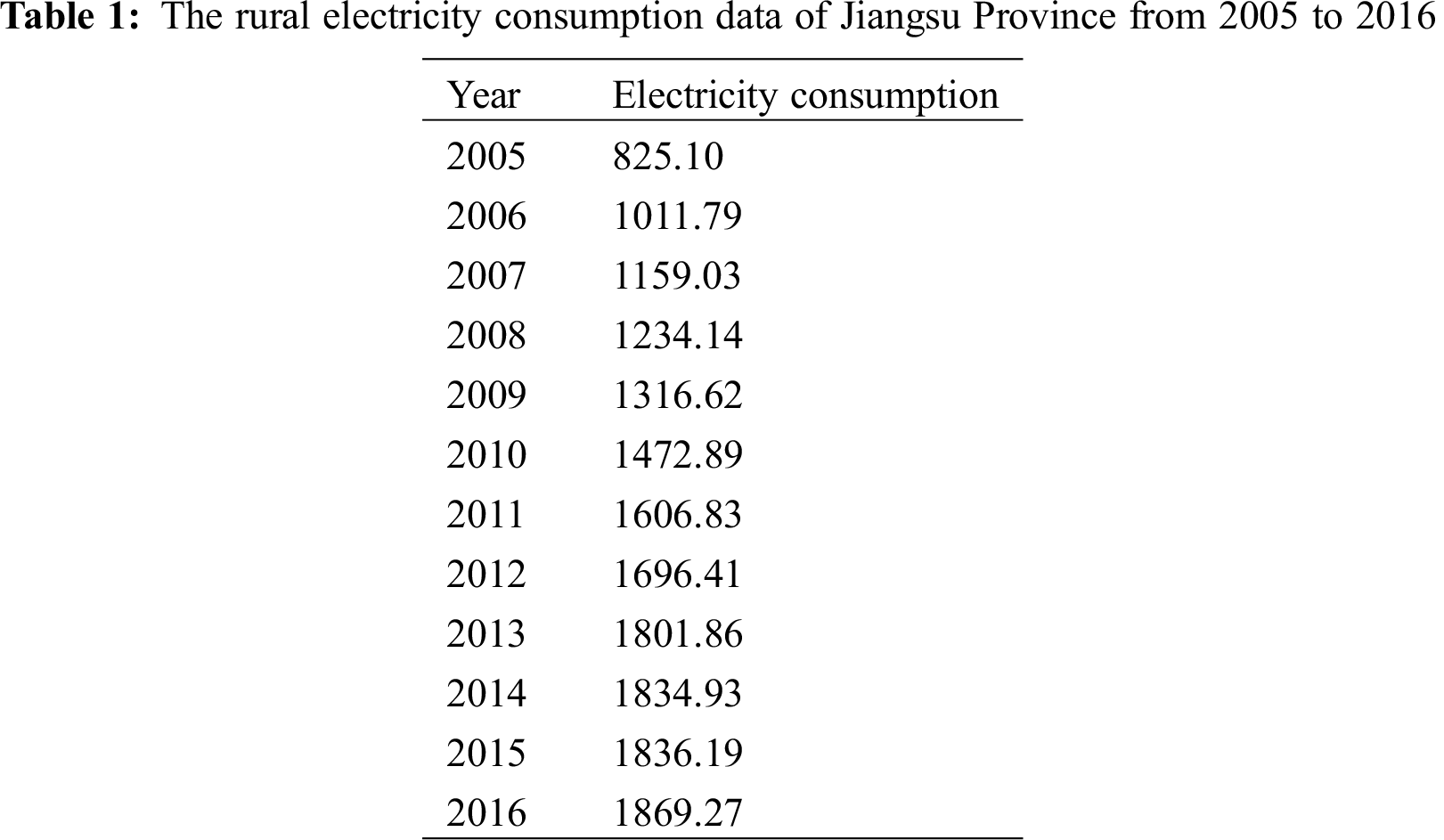
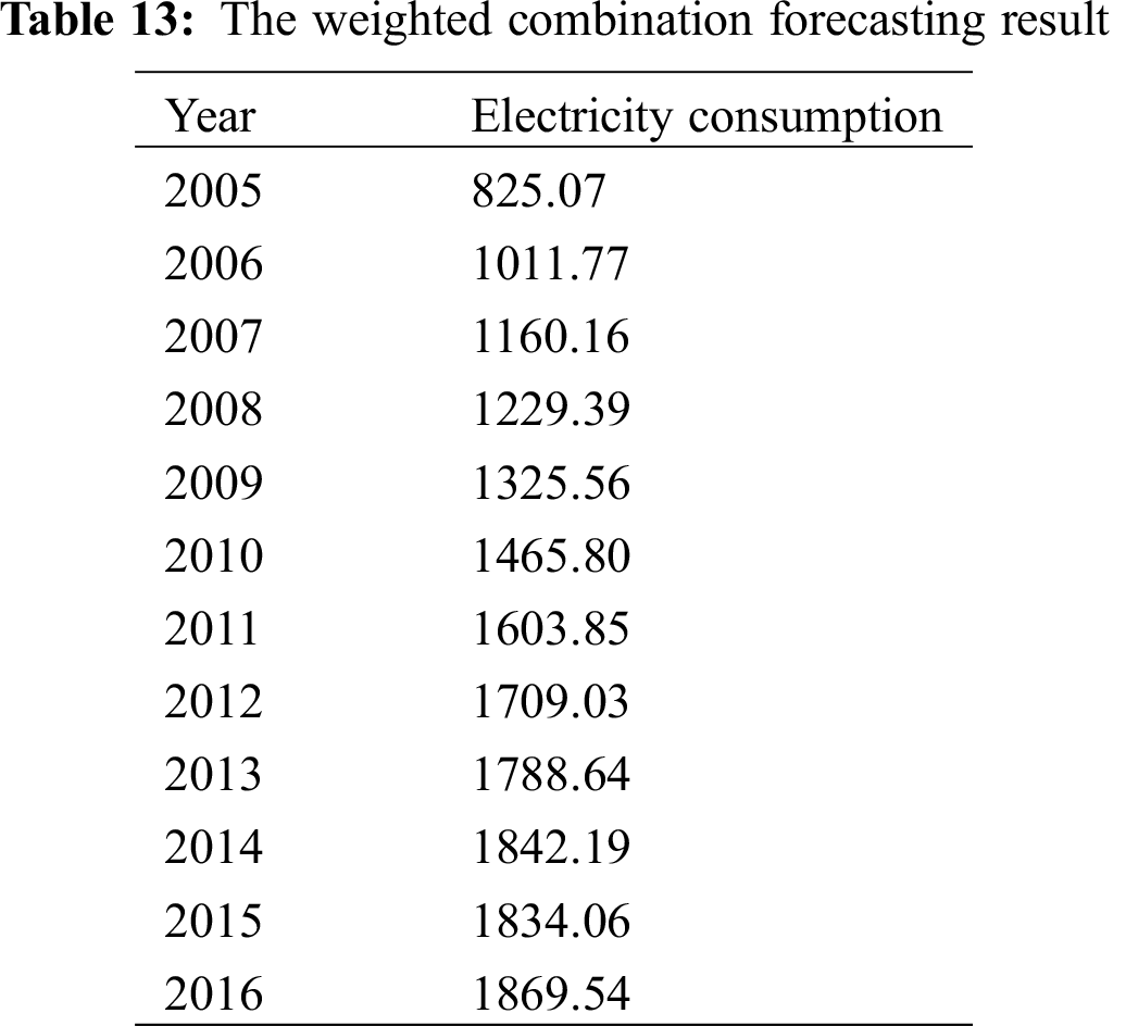
The rural electricity consumption data of Jiangsu Province from 2005 to 2016 are selected to establish the model. The data are from China Statistical Yearbook 2017 (Tab. 1), and the unit of electricity consumption in this paper is 100 million kWh. The years 2005 to 2015 are history years and 2016 is forecasting year. The electricity consumption of 2016 shown in Tab. 1 is taken as validation data.

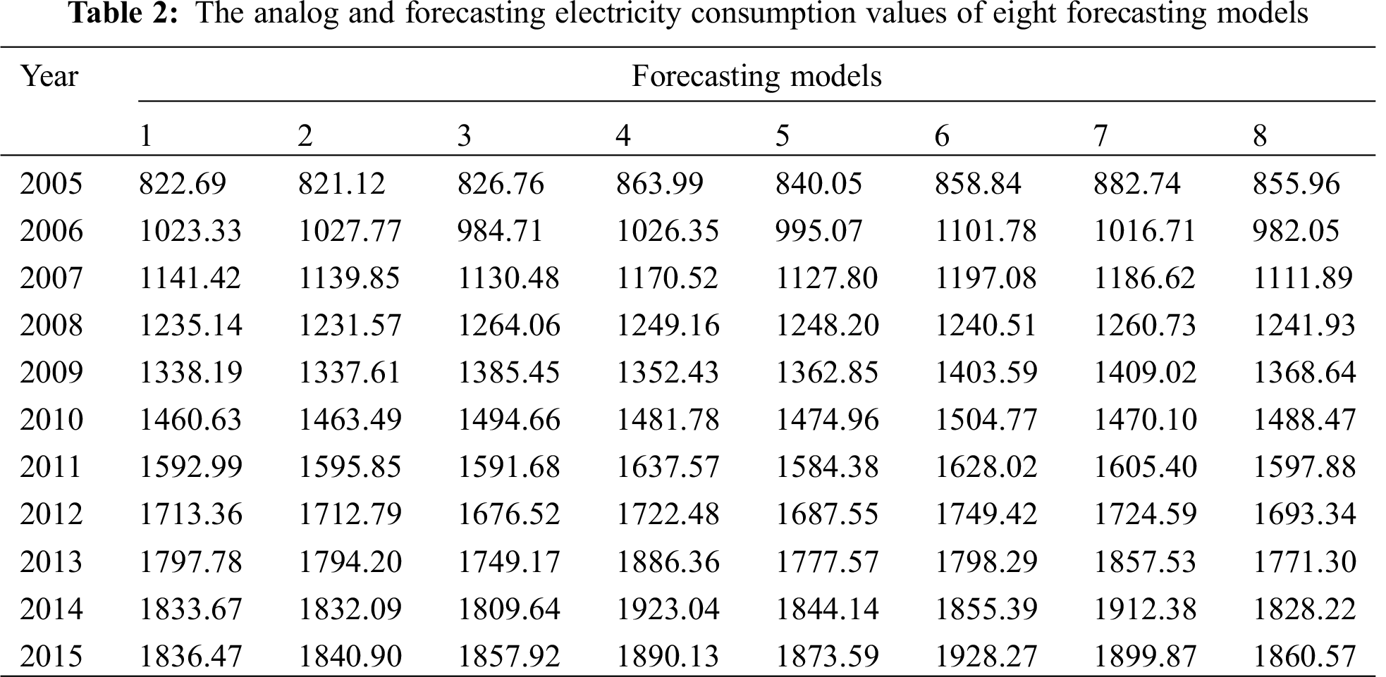
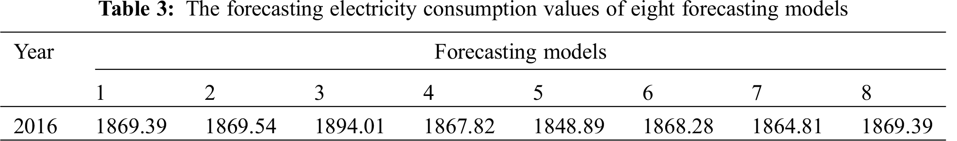
The initial forecasting models are (1) Hyperbola model; (2) COMPERTZ model; (3) Exponential model; (4) Power function model; (5) Cubic curve model; (6) S-curve model; (7) Logarithm model; (8) Para-curve model. Their analog and forecasting electricity consumption values are shown in Tabs. 2 and 3.

Assuming that analog effectiveness and forecasting effectiveness are equally important, λ = η = 0.5. According to the comprehensive effectiveness calculation approach based on Markov chain conversion and cloud model (Eq. (17)), the comprehensive effectiveness of each forecasting model is obtained as shown in Tab. 4.

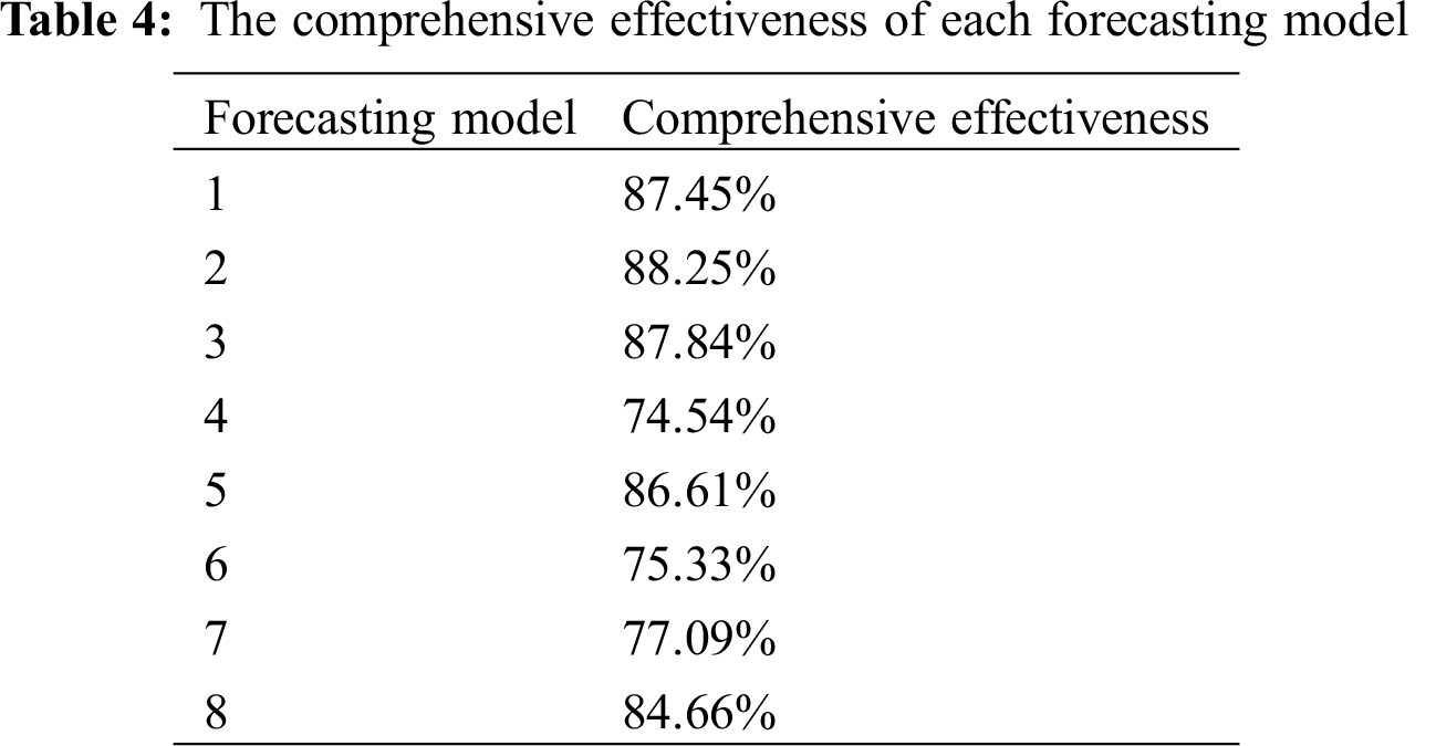
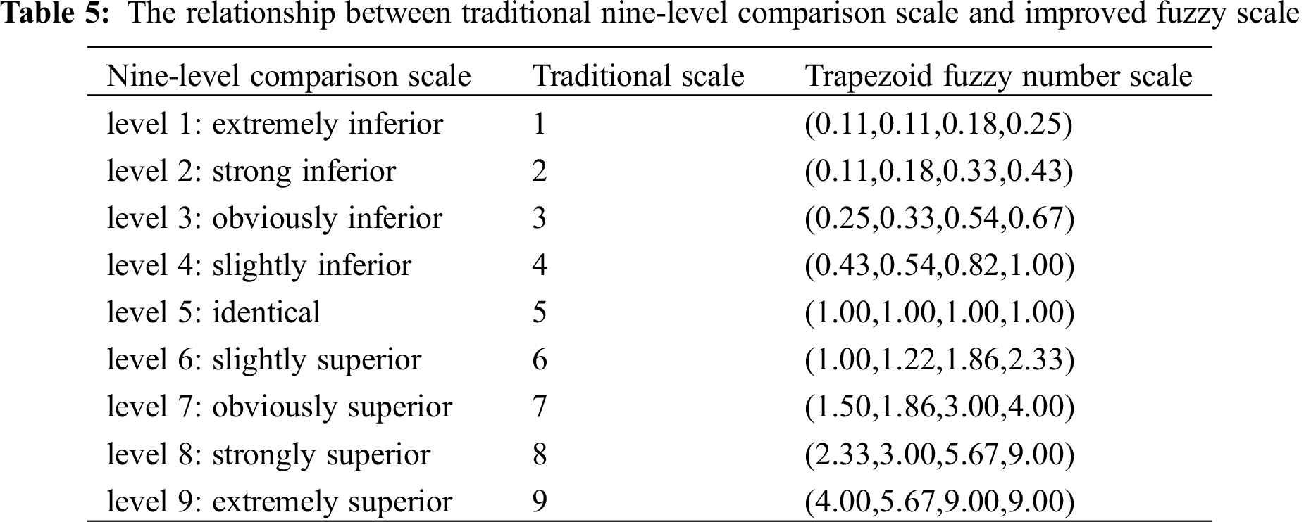
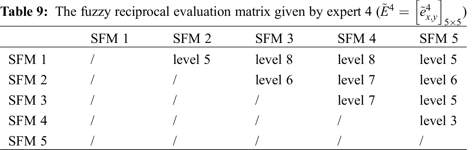
According to Eq. (19), the threshold value of forecasting model selection is 82.72%. Therefore forecasting models 1, 2, 3, 5 and 8 are selected for the subsequent combination forecasting. These models correspond to selected forecasting models (SFM) 1, 2, 3, 4 and 5 in turn. Based on the fuzzy scale joint evaluation method proposed in Section 4, it is assumed that there are four experts to determine the weight of selected forecasting model. This paper uses the trapezoid fuzzy number scale proposed in Reference [24,27] to express the evaluation score of expert. The traditional nine-level comparison scale is improved as shown in Tab. 5. For example, the scale value of comparison scale “level 2: Strong inferior” is 2, which can firstly be converted to 2/8. Then real number “2” corresponds to trapezoid fuzzy number (1, 1.5, 2.5, 3) while real number “8” corresponds to trapezoid fuzzy number (7, 7.5, 8.5, 9). Lastly based on the operation rules of trapezoid fuzzy number the trapezoid fuzzy number scale of “level 2: strong inferior” can be obtained as (0.11, 0.18, 0.33, 0.43), which is shown in Tab. 5.

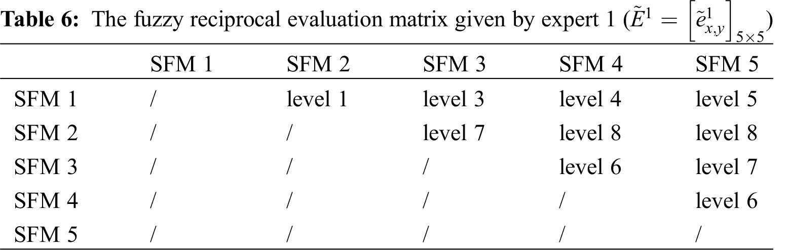
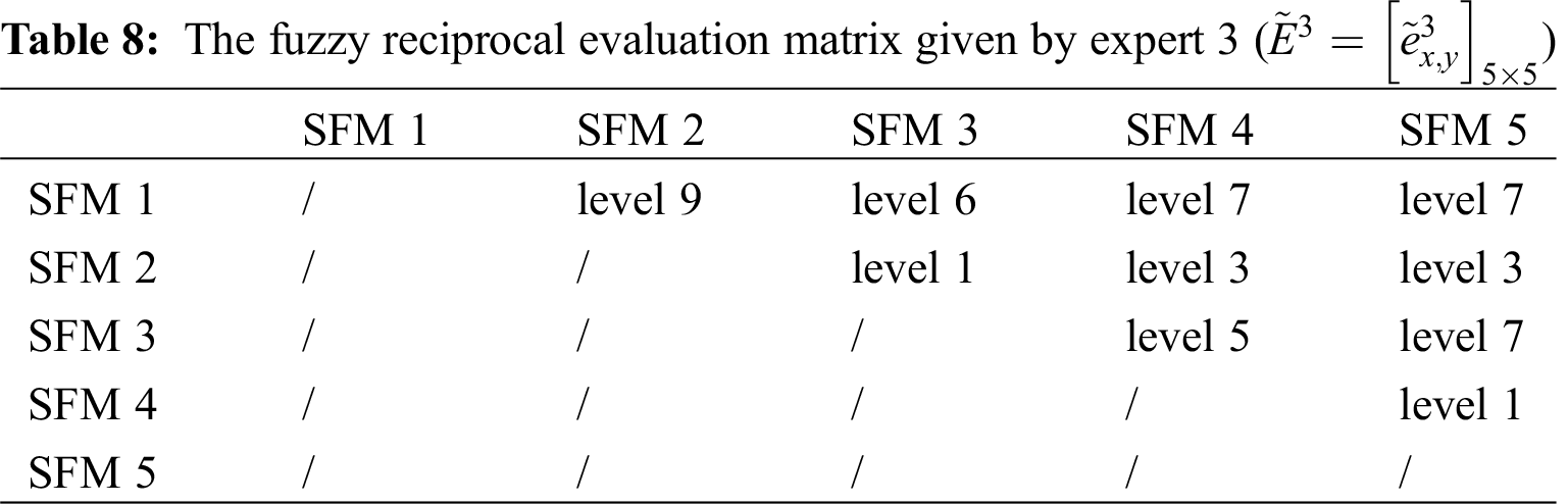
The fuzzy reciprocal evaluation matrices given by the four experts are shown in Tabs. 6, 7, 8 and 9.

Evaluation matrices E~1 , E~2 , E~4 and E~4 are qualified in consistency inspection according to the consistency inspection approach [24,27]. Then the joint evaluation matrix is constructed as E~=[e~x,y]5×5 and e~x,y={e~x,y1,e~x,y2,e~x,y3,e~x,y4} . For example, e~1,21 = (0.11,0.11,0.18,0.25), e~1,22 = (1.00,1.00,1.00,1.00), e~1,23 = (4.00,5.67,9.00,9.00), e~1,24 = (1.00,1.00,1.00,1.00), so e~1,2 = {(0.11,0.11,0.18,0.25),(1.00,1.00,1.00,1.00), (4.00,5.67,9.00,9.00), (1.00,1.00,1.00,1.00)}.

Next the rough boundary interval of e~1,2 is calculated according to Eqs. (22)–(27).

For e~1,21 in e~1,2 , the rough upper boundary is:

L_(e~1,21) = ((0.11,0.11,0.18,0.25) + (1.00,1.00,1.00,1.00) + (4.00,5.67,9.00,9.00) + (1.00,1.00,1.00,1.00))/4

= (1.53,1.94,2.79,2.81).

And the rough lower boundary is L¯(e~1,2) = (0.11,0.11,0.18,0.25)/1 = (0.11,0.11,0.18,0.25).

Then the rough boundary interval of e~1,21 in e~1,2 is obtained as RBI(e~1,21) = [(0.11,0.11,0.18,0.25), (1.53,1.94,2.79,2.81)]. By same way:

RBI(e~1,22) = [(0.70,0.70,0.73,0.75),(2.00,2.56,3.67,3.67)],

RBI(e~1,23) = [(1.53,1.94,2.79,2.81),(4.00,5.67,9.00,9.00)],

RBI(e~1,24) = [(0.70,0.70,0.73,0.75),(2.00,2.56,3.67,3.67)].

According to Eqs. (25)–(27), The rough boundary interval of e~1,2 is obtained as RBI(e~1,2) =[(0.76,0.86,1.11,1.14),(2.38,3.18,4.78,4.79)]. After calculating the rough boundary interval of all elements in E~=[e~x,y]5×5 , rough boundary interval evaluation matrix is constructed as shown in Tab. 10.

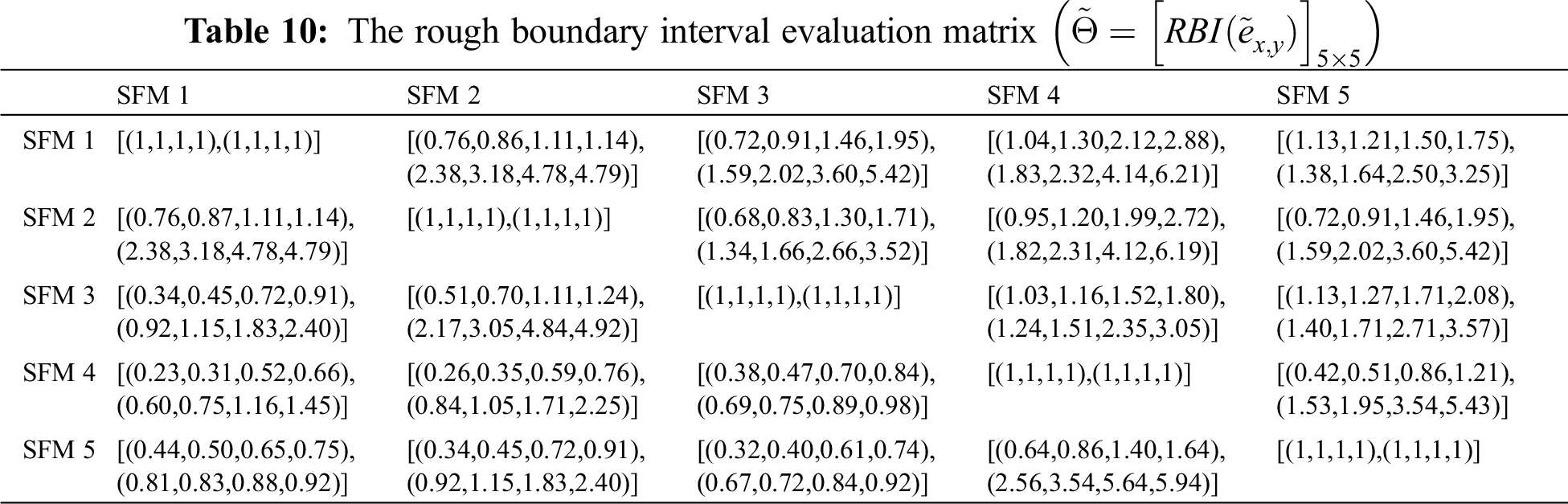
According to Eqs. (29) and (30), Θ~=[RBI(e~x,y)]5×5 is divided into two matrices as: Θ~_=[L_(e~x,y)]5×5 and Θ~¯=[L¯(e~x,y)]5×5 . As shown in Tabs. 11 and 12, Θ~_ and Θ~¯ are converted to Θ_ and Θ¯ which are real number form, respectively.

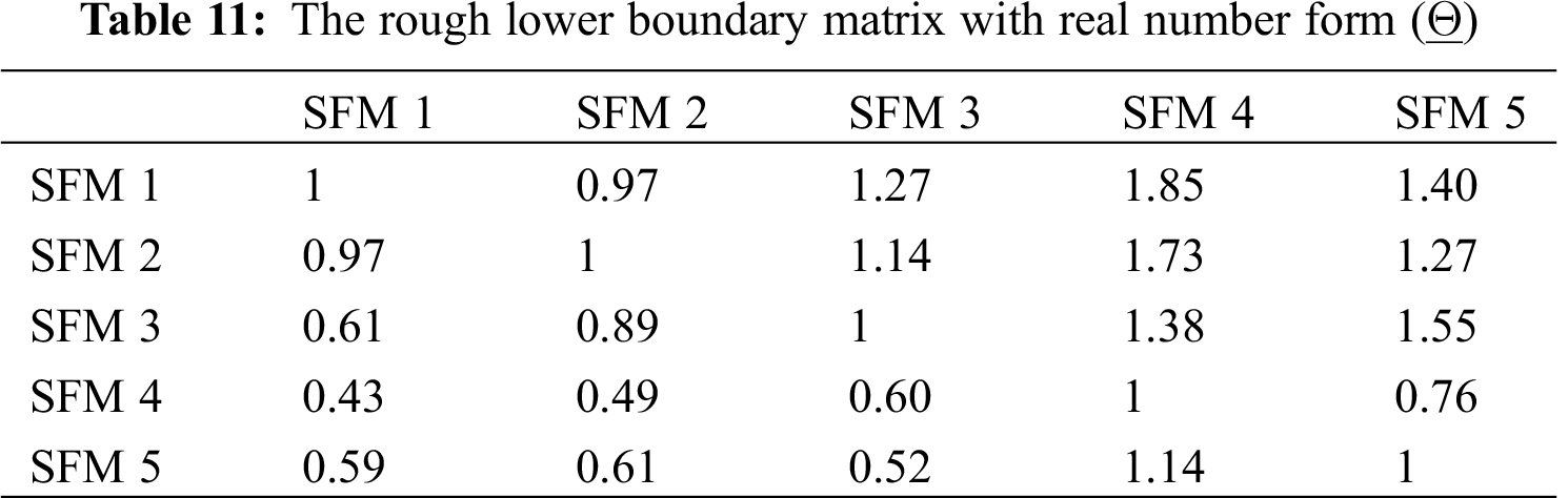
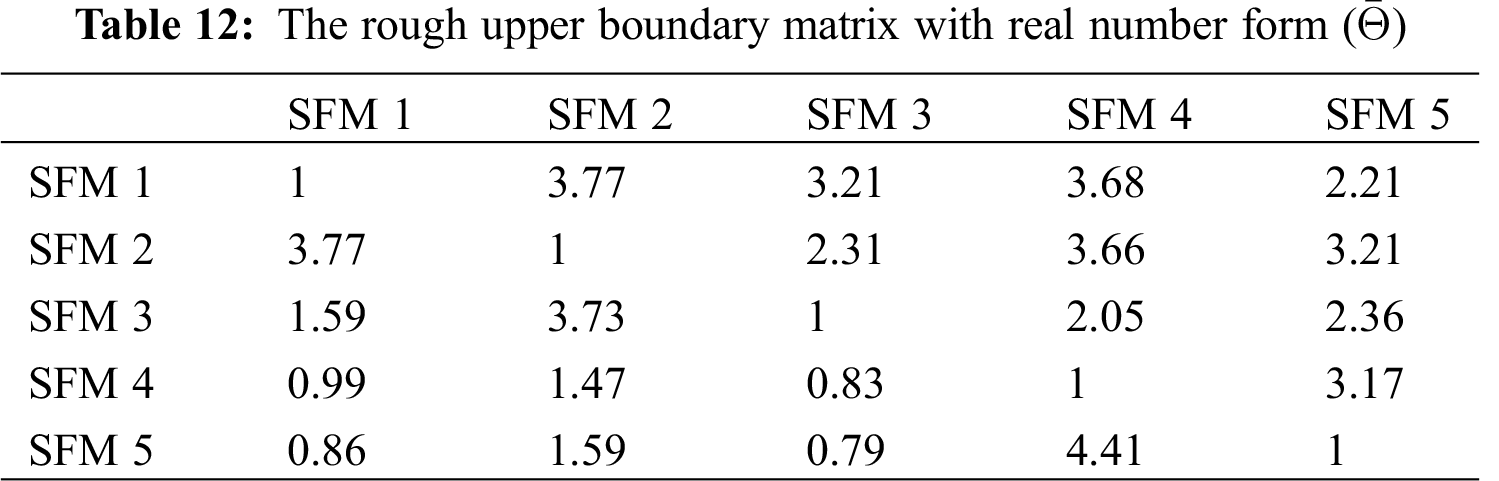
The eigenvectors of Θ_ and Θ¯ corresponding to maximum eigenvalues are obtained respectively as ω_ = [0.56,0.53,0.46,0.28,0.33]T and ω¯ = [0.56,0.55,0.45,0.29,0.31]T. According to Eqs. (33) and (34), the weight vector of five selected forecasting models is obtained as ω = [0.26,0.25,0.21,0.13,0.15]T. Then according to Eq. (35), the weighted combination forecasting result is obtained as shown in Tab. 13.

The percentage error (PE) of single forecasting models (SFM 1, 2, 3, 4 and 5) and weighted combination forecasting model are compared as shown in Tab. 14, while the mean absolute percentage error (MAPE) of single forecasting models (SFM 1, 2, 3, 4 and 5) and weighted combination forecasting model are compared as shown in Tab. 15.

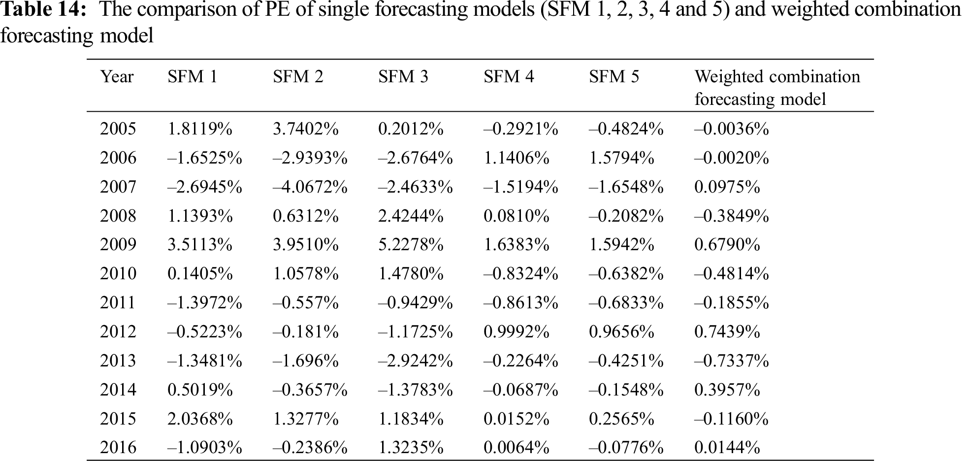
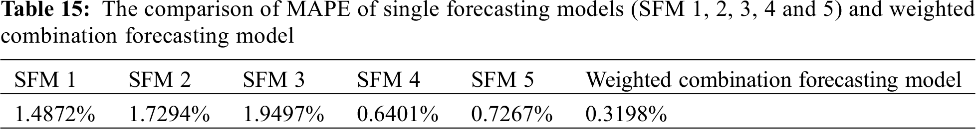
Figs. 2 and 3 are error analysis of single forecasting models (SFM 1, 2, 3, 4 and 5) and weighted combination forecasting model. As can be seen in Fig. 2, the maximum PEs of SFM 1, 2, 3, 4 and 5 are 3.5113%, –4.0672%, 5.2278%, 1.6383% and –1.6548%, respectively, while the maximum PE of weighted combination forecasting model is only 0.7439%, which is greatly reduced. In Fig. 3, the MAPE of weighted combination forecasting model is only 0.3198%. Compared with single forecasting models, the MAPE of weighted combination forecasting model is also greatly reduced.

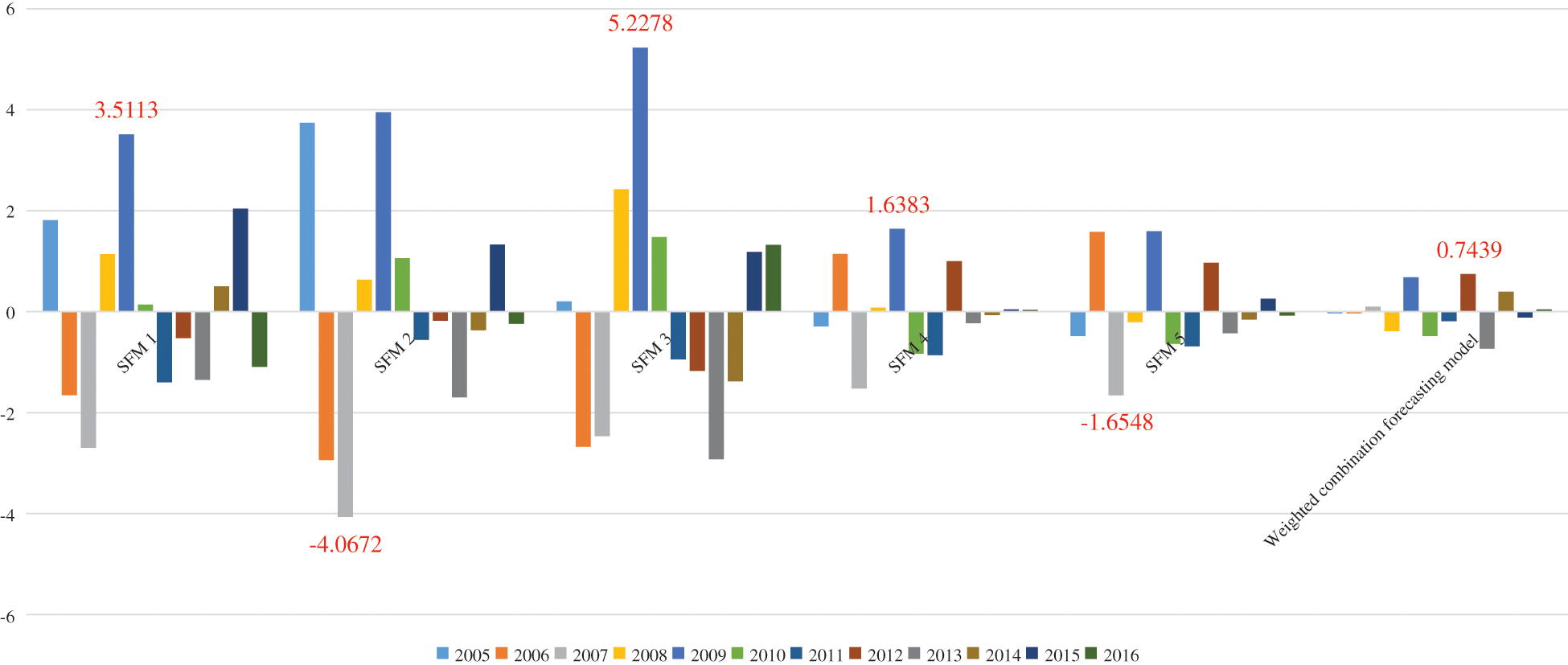
Figure 2: PE analysis

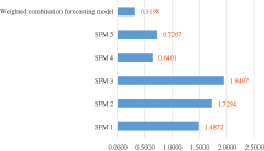
Figure 3: MAPE analysis

It can be seen that this weighted combination forecasting model can effectively improve the forecasting accuracy and increase the credibility of the model. In load forecasting with abundant historical information, combination forecasting model can synthesize information from various single models, which not only improves the accuracy of load forecasting, but also has strong operability.

6  Conclusions

The forecasting model selection is applied to weighted combination forecasting, and the rural electricity consumption data of a province in China is forecasted. The weighted combination forecasting results show that the forecasting indexes PE and MAPE are improved significantly compared with the single forecasting models. The forecasting accuracy has been greatly improved, proving that the forecasting method is effective and feasible, and has played a role in expanding the combined forecasting method. Compared with other combination methods, the weighted combination forecasting based on fuzzy scale joint evaluation method, which is based on the experience and wisdom of experts, is more practical and easier to implement. However, all experts are treated equal in the fuzzy scale joint evaluation. Obviously, the ability of experts is different and this problem will be considered in future work.

Funding Statement: The authors received no specific funding for this study.

Conflicts of Interest: The authors declare that they have no conflicts of interest to report regarding the present study.

References

 1.  Chen, Q., Jin, X., Yao, J., Yang, S., Gong, L. et al. (2014). Improved artificial bee colony algorithm applied to medium and long-term load combination forecasting. Power System Protection and Control, 23, 113–117. [Google Scholar]

 2.  Zhou, S., Zhou, R., Li, H., Li, S. (2015). Method of combine load forecast via information transformation and language evaluation. Proceedings of the Chinese Society of Universities for Electric Power System and Its Automation, 27(2), 20–26. [Google Scholar]

 3.  Jin, X., Luo, D., Sun, G., Zhang, H., Zheng, D. et al. (2012). Sifting and combination method of medium and long term load forecasting model. Proceedings of the Chinese Society of Universities for Electric Power System and Its Automation, 24(4), 150–156. [Google Scholar]

 4.  Sun, G., Yao, J., Xie, Y., Bu, H. (2009). Combination forecast of medium and long term load using fuzzy adaptive variable weight based on fresh degree function and forecasting availability. Power System Technology, 33(9), 103–107. [Google Scholar]

 5.  Yang, J., Ouyang, S., Shi, Y., Huang, R., Liu, Z. (2014). Combined membership function and its application on fuzzy evaluation of power quality. Advanced Technology of Electrical Engineering and Energy, 33(2), 63–69. [Google Scholar]

 6.  Huang, Y., Xu, Z., Liu, J., Zhou, R. (2005). Combining forecast based on fuzzy optimal selection of multi attributes semi structural decision-making. Electric Power, 38(9), 61–65. [Google Scholar]

 7.  Li, C., Niu, D., Meng, L. (2009). A comprehensive model for long- and medium-term load forecasting based on analytic hierarchy process and radial basis function neural network. Power System Technology, 33(2), 99–104. [Google Scholar]

 8.  Niu, D., Lu, H., Zhang, Y. (2008). Combination method of mid-long term load forecasting based on support vector machine within the Bayesian evidence framework. Journal of North China Electric Power University, 35(6), 62–66. [Google Scholar]

 9.  Xiao, X., Ge, J., He, D. (2008). Combination method of mid-long term load forecasting based on support vector machine. Proceedings of the Chinese Society of Universities for Electric Power System and Its Automation, 20(1), 84–88. [Google Scholar]

10. Ma, X., Yan, B., Tang, Y., Zhang, J. (2015). Medium and long-term load forecasting based on optimized combination forecast technology. Proceedings of the Chinese Society of Universities for Electric Power System and its Automation, 27(6), 62–67. [Google Scholar]

11. Jiang, Y., Wang, S., Feng, Y. (2012). Medium-long term power load forecasting based on recursive right combination model. Proceedings of the Chinese Society of Universities for Electric Power System and Its Automation, 24(1), 151–155. [Google Scholar]

12. Zhou, Q., Ren, H., Li, J., Zhang, Y., Zhou, Y. et al. (2010). Variable weight combination method for mid-long term power load forecasting based on hierarchical structure. Proceedings of the Chinese Society for Electrical Engineering, 30(16), 47–52. [Google Scholar]

13. You, S., Cheng, H., Xie, H., Guo, W., Lu, J. (2004). Application of combination forecasting by Fuzzy method in mid-and long-term load forecasting. Proceedings of the Chinese Society of Universities for Electric Power System and Its Automation, 16(3), 53–56. [Google Scholar]

14. Wilinski, A. (2019). Time series modeling and forecasting based on a Markov chain with changing transition matrices. Expert Systems with Applications, 133(7), 163–172. DOI 10.1016/j.eswa.2019.04.067. [Google Scholar] [CrossRef]

15. Arruda, E., Fragoso, M., Ourique, F. (2019). A multi-cluster time aggregation approach for Markov chains. Automatica, 99, 382–389. DOI 10.1016/j.automatica.2018.10.027. [Google Scholar] [CrossRef]

16. Zhu, C., Zhang, Y., Yan, Z., Zhu, J., Zhao, T. (2020). A wind power time series modeling method based on the improved Markov Chain Monte Carlo Method. Transactions of China Electrotechnical Society, 35(3), 577–589. [Google Scholar]

17. Wan, H., Ren, G. (2020). Study on the foundation pit settlement prediction model of logistic curve optimized by Markov Chain. Journal of Geomatics Science and Technology, 37(2), 166–170. [Google Scholar]

18. Wang, H., Liu, K., Zhu, H. (2016). Load forecasting of power system based on cloud model and support vector machine with RBF. Journal of Lanzhou University of Technology, 42(4), 85–88. [Google Scholar]

19. Li, H., Wei, M., Chen, Y., Lin, Z. (2016). Assessment method for power emergency group decision-making based on cloud model. Electric Power, 49(4), 42–48. [Google Scholar]

20. Wang, H., Liu, K., Yang, S. (2016). Load forecasting of power system based on cloud model SVM. Computer Systems & Applications, 25(5), 209–212. [Google Scholar]

21. Liu, D., Zhang, Q., Li, X., Gu, Y., Tan, Z. (2019). Identification of potential harmful behaviors in electricity market based on cloud model and fuzzy petri net. Automation of Electric Power Systems, 43(2), 25–33. [Google Scholar]

22. Yoder, M., Hering, A. S., Navidi, W. C., Larson, K. (2014). Short-term forecasting of categorical changes in wind power with Markov chain models. Wind Energy, 17, 1425–1439. [Google Scholar]

23. Wang, G., Xu, C., Li, D. (2014). Generic normal cloud model. Information Sciences, 280, 1–15. DOI 10.1016/j.ins.2014.04.051. [Google Scholar] [CrossRef]

24. Li, L., Mao, C., Lei, B., Gao, Y., Liu, Y. et al. (2020). Decision-making of product-service system solution selection based on integrated weight and technique for order preference by similarity to an ideal solution. IET Collaborative Intelligent Manufacturing, 2(3), 102–108. DOI 10.1049/iet-cim.2020.0003. [Google Scholar] [CrossRef]

25. Greco, S., Matarazzo, B., Slowinski, R. (2001). Rough sets theory for multicriteria decision analysis. European Journal of Operational Research, 129(1), 1–47. DOI 10.1016/S0377-2217(00)00167-3. [Google Scholar] [CrossRef]

26. Li, J., Fang, H., Song, W. (2019). Failure mode and effects analysis using variable precision rough set theory and TODIM method. IEEE Transactions on Reliability, 99, 1–15. [Google Scholar]

27. He, Y., Wei, C., Long, H., Raza Ashfaq, R., Huang, J. (2018). Random weight network-based fuzzy nonlinear regression for trapezoidal fuzzy number data. Applied Soft Computing Journal, 70(3), 959–979. DOI 10.1016/j.asoc.2017.08.006. [Google Scholar] [CrossRef]

This work is licensed under a Creative Commons Attribution 4.0 International License, which permits unrestricted use, distribution, and reproduction in any medium, provided the original work is properly cited.