| Energy Engineering |
DOI: 10.32604/EE.2021.014177
ARTICLE
Power Data Preprocessing Method of Mountain Wind Farm Based on POT-DBSCAN
Engineering Research Center of Hunan Province for the Mining and Utilization of Wind Turbines Operation Data, Hunan University of Science and Technology, Xiangtan, 411201, China
*Corresponding Author: Qiancheng Zhao. Email: qczhao@hnust.edu.cn
Received: 07 September 2020; Accepted: 20 October 2020
Abstract: Due to the frequent changes of wind speed and wind direction, the accuracy of wind turbine (WT) power prediction using traditional data preprocessing method is low. This paper proposes a data preprocessing method which combines POT with DBSCAN (POT-DBSCAN) to improve the prediction efficiency of wind power prediction model. Firstly, according to the data of WT in the normal operation condition, the power prediction model of WT is established based on the Particle Swarm Optimization (PSO) Arithmetic which is combined with the BP Neural Network (PSO-BP). Secondly, the wind-power data obtained from the supervisory control and data acquisition (SCADA) system is preprocessed by the POT-DBSCAN method. Then, the power prediction of the preprocessed data is carried out by PSO-BP model. Finally, the necessity of preprocessing is verified by the indexes. This case analysis shows that the prediction result of POT-DBSCAN preprocessing is better than that of the Quartile method. Therefore, the accuracy of data and prediction model can be improved by using this method.
Keywords: Wind turbine; SCADA data; data preprocessing method; power prediction
Wind energy is a kind of clean, pollution-free, and renewable green energy. As an important part of new energy, it has been paid close attention by countries all over the world. Many countries have taken the wind power generation as an important strategy for economic development [1,2]. On the basis of the statistics of the World Wind Energy Association, the newly installed global wind power capacity in 2019 was 59.7 GW, and the total installed capacity was close to 650 GW. China accounts for approximately 38% of the global total installed wind power capacity and has become currently the largest wind power market worldwide. Compared with the wind farms on the northern plain, the wind farms in southern China are characterized by strong randomness and instability because of the mountainous territory and complex turbulence, which will have a great impact on wind power integration and is not conducive to safe and reliable operation of the wind turbines (WTs) [3,4]. Operation experience of most wind farms shows that power prediction is the main way to solve this problem [5]. According to the prediction results of WT output, effective dispatching and scientific management of WTs can be carried out to improve the wind energy utilization rate of WTs and ensure the safe operation of power network [6,7].
The operation state of WT is mainly characterized by the power output, and the power curve reflects the performance characteristics and operational features of WT. According to the IEC 61400-12 Standard, the power curve of WT is the relation curve of output power with wind speed change, which is often used to evaluate the operational performance of WT [8,9]. In the actual operation process, there are large amount of abnormal data of wind speed power [10]. Without processing the abnormal data, using the actual measured wind speed power data for analysis will have a huge effect on the results [11].
There are mainly two categories of traditional data cleaning methods with low applicability. The first category is based on mathematical statistics. Shen et al. [12] proposed that under certain wind speed interval conditions, the Quartile method was used to determine the identification boundary of the out-of-limit wind-power data, and then out-of-limit abnormal data in the actual data set were identified and eliminated. Kusiak et al. [13] established a nonlinear model of the power curve to identify and filter abnormal data through the residual method and the control chart. Yue et al. [14] proposed the judgment method of “
Although the above methods such as machine learning can get more accurate data, they did not take into account the impact of the special working environment on the data. At the same time, because machine learning method mainly starts from the characteristics and structure of data, mining the depth and essential characteristics of data, it has been widely used in WT power prediction, with the common methods including SVM [22], neural network [23], gray prediction [24] and so on in recent years. Among them, artificial neural network has the characteristics of strong nonlinear fitting, adaptation and self-learning, and it is especially suitable for predicting wind-power. Such as, Sun et al. proposed the application of GA-ANN model in wind-power prediction [25]. Peng et al. [26] proposed a method for wind-power prediction based on artificial neural network and a hybrid strategy. Although the above direct use of DNN to predict the power can get more accurate results, there are problems of high calculation cost and slow training speed in searching the optimal parameters of the network model, which is not suitable for the nonlinear system with many parameters.
To solve the above problems, this paper proposes a WT power prediction method based on POT-DBSCAN preprocessing. The method not only obtains more accurate data, but also obtains more accurate prediction results by the PSO-BP algorithm, providing an effective early warning research method for the safe and reliable operation of WTs. This research can help the relevant departments of power system to accurately assess the risk of the power grid operation, formulate reasonable power generation plans, effectively reduce the operation cost of the power grid, and greatly promote the development of green energy.
2 Influence of Wind-Power Data
The WT generator is to convert the changing wind energy into mechanical energy, then transform the mechanical energy to electric energy and transport it to the power network. When the wind speed is between the cut in wind speed and the rated wind speed, wind power can be evaluated by the following equation [27]:
where
As shown in Fig. 1, an obvious abnormal data exists in the actual measurement data. According to the characteristics of abnormal data distribution, the operation data of WT can be divided into outlier data, power limit data, deviating cluster data and abnormal stoppage data [28]. The distribution of outlier data in the scatter diagram is discrete, isolated and far from the power curve, which is due to the large data error caused by the sensor anomalies and failures. The deviation cluster data are distributed on the power curve with high density and small range, which is mainly caused by the electromagnetic interference or computer information processing and storage failure for a long time.

Figure 1: Raw WT power curve with operating interference
Some abnormal data may also be due to the sudden change of wind speed, resulting in serious wind speed rising or falling edge. The calculation method of 10-min average compression processing will result in the data fluctuating along and deviating from the power curve, which leads to inaccuracy of the data. A period of wind speed rise stage data using the IEC 61400 Standard Bin method is selected to draw the power curve as shown in Fig. 2. It can be seen from the figure that there are some power points that deviate from the power curve through the 10-min average compression processing calculation method. Taking the red point in the figure as an example, with the sudden increase of wind speed, the power is also increasing. Because there are many data with small power value in 10-min, the average calculated power value will be pulled down and located at the bottom of the power curve. So, the data obtained by the 10-min average compression processing method is not accurate in the process of sudden change of wind speed. With the POT method, the power value can be corrected through multiplying the average value of 10-min by the data within the threshold range. Therefore, this paper proposes a data preprocessing method for POT-DBSCAN.

Figure 2: Power diagram at wind speed rising stage
3 Wind-Power Data Preprocessing Methods
In addition to the data collected by SCADA system, there are also some abnormal data, which are caused by complex environmental changes and sensor failures. Therefore, before modeling and analyzing the WT units, it is necessary to preprocess the data. In this paper, the POT-DBSCAN method is used to preprocess the data.
Let the independent identically distributed random variables be
The distribution of excess numbers is known by the Pickands-Balkama-de Hean Theorem. For a sufficiently large threshold, the distribution function of excess values approximately follows the Generalized Pareto Distribution (GDP). The GDP of the excess distribution is approximately expressed as:
when
when
when the threshold is determined,
The DBSCAN clustering differs from other clustering algorithms in that it classifies clusters according to the density distribution of data sets. It cannot only deal with noise effectively but also cluster arbitrary shape data. The core principle of DBSCAN clustering algorithm is that every point exists in the database. When the density of the points in the adjacent area is greater than a certain set threshold, the data sets will be added to the adjacent class and then repeated clustering is continued. The DBSCAN clustering method, a typical clustering method based on density, can identify a cluster by setting a density threshold. This clustering algorithm has two key parameters—Eps and Minpts. Eps represents the radius of a cluster, and Minpts is the number of neighbors within the cluster. With references [29,30], Minpts is set to 4 in this study, and Eps is calculated using the following equation:
where m denotes the number of objects in the experimental data set, n is the dimensionality of the experimental space,
where
3.3 Wind-Power Data Preprocessing Process
There are various sources of abnormal data of the WT. If the SCADA data containing abnormal data are directly used in the WT power prediction, large errors will be produced. Because the operation state of a WT is easily affected by the abnormal data, it is necessary to preprocess the abnormal data before analysis so as to avoid the influence of abnormal data on the prediction model of the WT. In this paper, the high-frequency data of the wind speed and power are all processed by the POT method to get 10-min data. The specific process is as follows: First, the high-frequency data corresponding to each 10-min data are filtered by the POT method. The filtering rule is taking the average value of each 10-min data which are multiplied by the positive and negative

Figure 3: The process of wind-power data preprocessing
4 PSO-BP Power Prediction Model
4.1 Particle Swarm Optimization BP Neural Network Algorithm
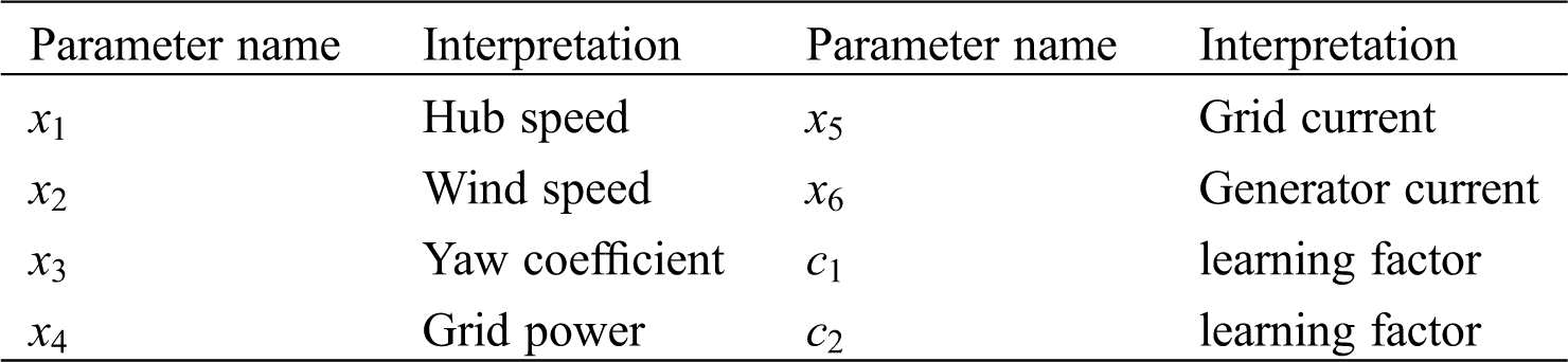
Although the PSO cannot realize adaptive learning and has slow convergence speed and poor robustness, it has strong global optimization ability. If the PSO-BP neural network algorithm is used, it can not only solve the problem that the BP neural network is easy to fall into local optimization and slow training speed, but also can fill the shortage of the PSO Algorithm. The topology of the BP neural network is shown in Fig. 4. The structure of the BP neural network is set as 6-6-1, and the number of training, the learning rate and the error target are 100, 0.1 and 0.0001 respectively. The input layers x1,x2,x3,x4,x5,x6 of the BP neural network represent the hub speed, wind speed, yaw coefficient, grid power, grid current, generator current respectively, and Y of the output layer represents power. The interpretation of every model parameter is shown in Tab. 1.

Figure 4: The topology of the BP neural network
Table 1: Interpretation of model parameters
The performance of the BP neural network prediction will be greatly affected by the setting of weights and thresholds. The PSO Algorithm can be used for global optimization to find the optimal combination of the neural network weights and thresholds. Then the BP neural network with optimized parameters can be used to predict the unit power, which can better improve the prediction performance. The flowchart of the PSO-BP is shown in Fig. 5, and the specific steps are as follows:
(1) The BP neural network is created, and the weights and thresholds of the neural network are initialized.
(2) Set parameters such as the transfer functions, number of training iterations, training error target, learning rate, etc. for the implicit and output layers of the network.
(3) Normalize the input and output data in the training sample.
(4) Set the parameters of PSO algorithm, and randomly generate the position and speed of each particle.
(5) The fitness function is constructed to optimize the weights and thresholds of the neural network.
(6) The fitness value of each particle is calculated to find the best position of individual and global.
(7) The velocity and position of particles are updated according to the correspondent updating equation.
(8) Increase the number of iterations to determine whether the iteration conditions are met. If they are met, stop and output the optimal weight and the threshold value. Otherwise, go to Step (6).
(9) The optimal weights and thresholds obtained from Step (8) are used to train the BP neural network.

Figure 5: Flowchart of PSO-BP neural network algorithm
4.2 Construction of Prediction Model Based on PSO-BP Algorithm
Based on the above theory, the data are preprocessed by the POT-DBSCAN Algorithm, and then the key parameters in the preprocessed data set are selected as the input of the PSO-BP neural network to establish the power prediction model to predict the power of WT. Accuracy is the most important factor to measure the effect of wind power prediction, and the main indexes of evaluating accuracy are the Root Mean Square Error (RMSE), the Mean Absolute Error (MAE), the Root Mean Square Percentage Error of Relative Error (RRMSE) and the Entropy [31,32].The formulas of these indexes are listed in (8), (9), (10) and (11). Where
where xi is a random event that may occur and Pi is the probability of the occurrence of the event xi. The flowchart of this study is displayed in Fig. 6 and the main process and steps involved are listed subsequently.
Stage 1: Data Preprocessing
The wind-power data are processed to the high-frequency data by the POT Method, and then the obvious outlier data are filtered by the DBSCAN clustering method.
Stage 2: Establishment of the PSO-BP Prediction Model
The PSO-BP Prediction Model is established by selecting the data of the hub speed, the wind speed, the yaw coefficient, the grid power, the grid current and the generator current in the normal working state of the SCADA system.
Stage 3: Verify the Effectiveness of the POT-DBSCAN Preprocessing Method
The preprocessed data are used for the power prediction through the PSO-BP Model, and the necessity of preprocessing is verified by the MAE, RMSE, RRMSE and the entropy error.

Figure 6: Flowchart of proposed in this study
The SCADA data used in this study are derived from the 2 MW permanent magnet direct-driven WTs, located in a mountainous wind farm in Southern China. The WT has a diameter of 96 m, a cut-in wind speed of 3 m/s, a rated wind speed of 11 m/s, and a rated power of 2000 KW. The SCADA System records 10-min average values under 1 Hz sampled WT condition and with external environment parameters, including the wind speed, the rotational speed, the current, the power, and so on. The SCADA data of WT No. 1, under the normal operation within 3 to 4 months in 2017, are selected to establish the prediction model. The model has 6-dimensional input and 1-dimensional output, so the number of selected data set is 7200 × 7 groups. According to the size of cut-in wind speed and rated wind speed, the data set is divided into eight parts. In each part, sample data are selected randomly with the ratio of 8:1. And there are totally 900 × 7 groups of sample data. Then 600 × 7 groups of training sample data and 300 × 7 groups of test sample data are selected with the ratio of 2:1. Finally, the accuracy test of the predicted value of the test sample power obtained by the model and the actual value is shown in Fig. 7. The calculated RRMSE was 1.77%, the calculated entropy was 2.69, and the correlation coefficient was 0.996. It can be found that the fitting effect of this model is better, so this model can meet the requirement of precision.

Figure 7: Comparison between the predicted value and the actual value of the test sample
Fig. 8 shows the annual wind-power scatter diagram of WT No. 1 in 2017. First, the high-frequency data corresponding to the 10-min data collected by SCADA system are processed by the POT method. Next, the processed data are saved as a new data set. Then, the new data set is further processed by the DBSCAN clustering method to generate the final data. Fig. 9 is obtained by using the POT-DBSCAN data preprocessing method.
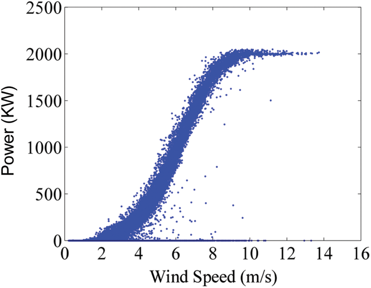
Figure 8: Actual measurement wind-power data

Figure 9: Wind-power data after preprocessing
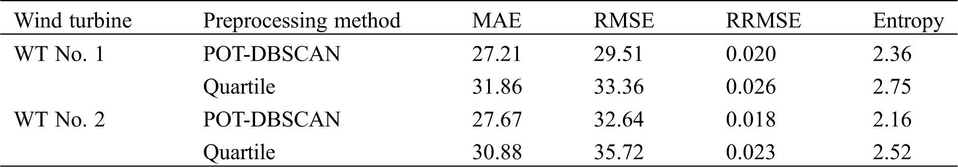
In this experiment, the prediction model is used to predict the power of the WTs. Since there are outlier data, data preprocessing is required to filter all abnormal data points. In recent studies, many excellent data preprocessing methods have been proposed. The Quartile method does not rely on the mean and variance to detect outliers, nor does it need the sequence to follow a certain distribution model. When the proportion of outliers is small, the data identification will be good enough. In this paper, the prediction model of quartile data preprocessing is selected as the benchmark model. In order to verify the superiority and effectiveness of the proposed POT-DBSCAN, the benchmark model is compared with the prediction model after data preprocessing by the POT-DBSCAN. The results are shown in Tab. 2. From the error results in the table, it can be concluded that the prediction effect of the POT-DBSCAN is better. The two methods will be further analyzed later.
Table 2: Prediction results of two preprocessing methods
Under the condition of normal operation, data from WT No. 1 within the two months after August 10th, 2017 and data form WT No. 2 within the two months before October 6th, 2017 are selected for analysis. The power prediction model of the PSO-BP is established by using the data of the POT-DBSCAN and Quartile preprocessing respectively. A subsequent case analysis also shows that setting a lower threshold for prediction model can more effectively predict an upcoming stoppage of the WTs (the MAE, RMSE, RRMSE and the entropy are 50, 50, 0.03 and 3 respectively, which are the effective lower thresholds for the WTs involved in this study). Fig. 10 shows the power prediction error results of the No. 1 WT two months after August 10. According to the trend of the MAE curve in this figure, the MAE values after the POT-DBSCAN preprocessing are all below 50, while the Mae values after the Quartile preprocessing are higher than 50. Similarly, the RMSE and entropy of the POT-DBSCAN preprocessing were below 50 and 3, while the RMSE and entropy were higher than the threshold after the Quartile preprocessing. After the POT-DBSCAN preprocessing, the RRMSE values were lower than 0.03, and the RRMSE values after the Quartile preprocessing were higher than 0.03.

Figure 10: Results of power prediction error of No. 1 WT
Fig. 11 shows the power prediction error results of the No. 2 WT in the two months before October 6. According to the trend of the MAE curve after the POT-DBSCAN preprocessing, the MAE values are all below 50. According to the trend chart of the root mean square error curve after the POT-DBSCAN preprocessing, RMSE values are all below 50. After the POT-DBSCAN preprocessing, RRMSE and entropy values were less than 0.03 and 3. It can be concluded from this figure that after the Quartile preprocessing, the four indicators are higher than the threshold for some time. These results verify the accuracy of the threshold value. Therefore, it can be considered that the WT operating state is better when the MAE, RMSE, RRMSE and the entropy value are below the threshold value of 50, 50, 0.03 and 3 respectively, which is consistent with the results of the normal operation of WT. The MAE, RMSE, RRMSE and the entropy are all lower than the threshold value from the trend chart of indicators pretreated by the POT-DBSCAN. However, from the trend chart of the MAE, RMSE, RRMSE and the entropy after the Quartile preprocessing, it can be seen that the indexes of some days are obviously higher than the threshold value. Because the normal working state of WT is selected, it is unreasonable to have such a phenomenon. Therefore, according to the above numerical results, the POT-DBSCAN method proposed in this paper is superior to the Quartile method. Both Quartile method and DBSCAN method are used to preprocess the 10-min data after averaging, and do not take the impact of sudden change of wind speed on the high-frequency data into consideration, while the POT method can better process the high-frequency data. Thus, it has also been verified that this data preprocessing method can improve the accuracy of the power prediction and is more effective.

Figure 11: Results of power prediction error of No. 2 WT
Aiming at the strong nonlinear relationship of the wind-power data caused by frequent changes of wind speed, a wind-power data preprocessing method based on the POT-DBSCAN is proposed in this paper. First, the power prediction model of WT based on the PSO-BP method is established by using the data collected under the normal operation. Then, the accuracy of the threshold is verified by calculating the MAE, RMSE, RRMSE and the entropy. Finally, through the prediction model analysis of the two WTs, it has been concluded that the indexes of the model after data POT-DBSCAN preprocessing are less than the threshold value, which is consistent with the results of the WT data under the normal operation condition. Data from the forecast model indicator trend chart that have been Quartile data preprocessed can be found to be higher than the threshold for a certain number of days. This is contrary to the result of the WT in normal working state. The results show that the POT-DBSCAN is more effective than the Quartile method. Because the Quartile preprocessing method does not consider the impact of frequent changes in wind speed on high-frequency data, but the POT-DBSCAN method can better solve this problem.
This paper proposes a method for the WT data preprocessing. The frequent changes of wind speed and direction not only affect the reliability of the WT, but also are not conducive to the accurate use of the SCADA data. The POT-DBSCAN preprocessing method proposed in this paper can improve the accuracy of data and prediction models. However, only the wind speed and power are considered in the current method. Wind direction and temperature also have great influence on the power of WT, which should be take into consideration in further studies.
Acknowledgement: The authors are thankful to the Engineering Research Center of Hunan Province for the Mining and Utilization of Wind Turbines Operation Data, Hunan University of Science and Technology, Xiangtan, China, for its extended support in using the facilities available at laboratory.
Funding Statement: This research was supported by National Natural Science Foundation of China (Nos. 51875199 and 51905165), Hunan Natural Science Fund Project (2019JJ50186), the Key Research and Development Program of Hunan Province (No. 2018GK2073).
Conflicts of Interest: The authors declare that they have no conflicts of interest to report regarding the present study.
1. Amirat, Y., Benbouzid, M. E. H., Al-Ahmar, E., Bensa, B., Turri, S. (2009). A brief status on condition monitoring and fault diagnosis in wind energy conversion systems. Renewable and Sustainable Energy Reviews, 13(9), 2629–2636. DOI 10.1016/j.rser.2009.06.031. [Google Scholar] [CrossRef]
2. Márquez, F. P. G., Tobias, A. M., Pérez, J. M. P., Papaelias, M. (2012). Condition monitoring of wind turbines: Techniques and methods. Renewable Energy, 46, 169–178. DOI 10.1016/j.renene.2012.03.003. [Google Scholar] [CrossRef]
3. Zhou, Q., Wang, C., Zhang, G. (2019). Hybrid forecasting system based on an optimal model selection strategy for different wind speed forecasting problems. Applied Energy, 250, 1559–1580. DOI 10.1016/j.apenergy.2019.05.016. [Google Scholar] [CrossRef]
4. Estefania, A., Sergio, M. M., Andrés, H. E., Emilio, G. L. (2018). Wind turbine reliability: A comprehensive review towards effective condition monitoring development. Applied Energy, 228, 1569–1583. DOI 10.1016/j.apenergy.2018.07.037. [Google Scholar] [CrossRef]
5. Noorollahi, Y., Yousefi, H., Mohammadi, M. (2016). Multi-criteria decision support system for wind farm site selection using GIS. Sustainable Energy Technologies and Assessments, 13, 38–50. DOI 10.1016/j.seta.2015.11.007. [Google Scholar] [CrossRef]
6. Chehouri, A., Younes, R., Ilinca, A., Perron, J. (2015). Review of performance optimization techniques applied to wind turbines. Applied Energy, 142, 361–388. DOI 10.1016/j.apenergy.2014.12.043. [Google Scholar] [CrossRef]
7. Li, J. L., Zhang, X. R., Zhou, X., Lu, L. Y. (2019). Reliability assessment of wind turbine bearing based on the degradation-Hidden-Markov model. Renewable Energy, 132, 1076–1087. DOI 10.1016/j.renene.2018.08.048. [Google Scholar] [CrossRef]
8. IEC, IEC 61400-12-1. (2005). Wind Turbines—Part 12-1: Power performance measurements of electricity producing wind turbines. International Electrotechnical Commission: Geneva, Switzerland. [Google Scholar]
9. Taslimi-Renani, E., Modiri-Delshad, M., Elias, M. F. M., Rahim, N. A. (2016). Development of an enhanced parametric model for wind turbine power curve. Applied Energy, 177, 544–552. DOI 10.1016/j.apenergy.2016.05.124. [Google Scholar] [CrossRef]
10. Dai, J. C., Liu, D. S., Wen, L., Long, X. (2016). Research on power coefficient of wind turbines based on SCADA data. Renewable Energy, 86, 206–215. DOI 10.1016/j.renene.2015.08.023. [Google Scholar] [CrossRef]
11. Swapna, S., Niranjan, P., Srinivas, B., Swapna, R. (2016). Data cleaning for data quality. IEEE International Conference on Computing for Sustainable Global Development. New Delhi, India. [Google Scholar]
12. Shen, X., Fu, X., Zhou, C. (2019). A combined algorithm for cleaning abnormal data of wind turbine power curve based on change point grouping algorithm and quartile algorithm. IEEE Transactions on Sustainable Energy, 10(1), 46–54. DOI 10.1109/TSTE.2018.2822682. [Google Scholar] [CrossRef]
13. Kusiak, A., Zheng, H. Y., Song, Z. (2009). Models for monitoring wind farm power. Renewable Energy, 34(3), 583–590. DOI 10.1016/j.renene.2008.05.032. [Google Scholar] [CrossRef]
14. Yue, W., David, G. I., Bruce, S., Stuart, J. G. (2014). Copula-based model for wind turbine power curve outlier rejection. Wind Energy, 17(11), 1677–1688. DOI 10.1002/we.1661. [Google Scholar] [CrossRef]
15. Zhao, Y., Lehman, B., Ball, R., Mosesian, J., Palma, J. F. D. (2013). Outlier detection rules for fault detection in soar photovoltaic arrays. Proceedings of the 28th Annual IEEE Applied Power Electronics Conference and Exposition, pp. 2913–2920, Long Beach, CA, USA: IEEE. [Google Scholar]
16. Zheng, L., Hu, W., Min, Y. (2015). Raw wind data preprocessing: A data-mining approach. IEEE Transactions on Sustainable Energy, 6(1), 11–19. DOI 10.1109/TSTE.2014.2355837. [Google Scholar] [CrossRef]
17. Sun, P., Li, J., Wang, C., Lei, X. (2016). A generalized model for wind turbine anomaly identification based on SCADA data. Applied Energy, 168, 550–567. DOI 10.1016/j.apenergy.2016.01.133. [Google Scholar] [CrossRef]
18. Wang, L., Zhang, Z., Long, H., Xu, J., Liu, R. (2017). Wind turbine gearbox failure identification with deep neural networks. IEEE Transactions on Industrial Informatics, 13(3), 1360–1368. DOI 10.1109/TII.2016.2607179. [Google Scholar] [CrossRef]
19. Santos, P., Villa, L. F., Reñones, A., Bustillo, A., Maudes, J. (2015). An SVM-based solution for fault detection in windturbines. Sensors, 15(3), 5627–5648. DOI 10.3390/s150305627. [Google Scholar] [CrossRef]
20. Schlechtingen, M., Santos, I. F., Achiche, S. (2013). Using data-mining approaches for wind turbine power curve monitoring: A comparative study. IEEE Transactions on Sustainable Energy, 4(3), 671–679. DOI 10.1109/TSTE.2013.2241797. [Google Scholar] [CrossRef]
21. Wu, X., Wu, B., Sun, J., Li, M. (2015). A possibilistic fuzzy c-means clustering algorithm. International Journal of Food Engineering, 13(1), 517–530. [Google Scholar]
22. Simani, S., Alvisi, S., Venturini, M. (2019). Data-driven control techniques for renewable energy conversion systems: Wind turbine and hydroelectric plants. Electronics, 8(2), 237. DOI 10.3390/electronics8020237. [Google Scholar] [CrossRef]
23. Schlechtingen, M., Santos, I. F. (2014). Wind turbine condition monitoring based on SCADA data using normal behavior models. Part 2: Application examples. Applied Soft Computing, 14, 447–460. DOI 10.1016/j.asoc.2013.09.016. [Google Scholar] [CrossRef]
24. Zhang, Y., Li, M., Dong, Z. Y., Meng, K. (2019). A probabilistic anomaly detection approach for data-driven wind turbine condition monitoring. International Journal of Electrical Power Energy Systems, 5, 149–158. [Google Scholar]
25. Sun, P., LI, J., Yan, Y., Lei, X., Zhang, X. (2015). Wind turbine anomaly detection using normal behavior models based on SCADA data. International Conference on High Voltage Engineering and Application, Poznan, Poland. [Google Scholar]
26. Peng, H., Liu, F., Yang, X. (2013). A hybrid strategy of short term wind power prediction. Renewable Energy, 50, 590–595. DOI 10.1016/j.renene.2012.07.022. [Google Scholar] [CrossRef]
27. Xiao, Z., Zhao, Q. C., Yang, X. B., Zhu, A. F. (2020). A power performance online assessment method of a wind turbine based on the probabilistic area metric. Applied Sciences, 10(9), 3268. [Google Scholar]
28. Schlechtingen, M., Santos, I. F. (2011). Comparative analysis of neural network and regression based condition monitoring approaches for wind turbine fault detection. Mechanical Systems & Signal Processing, 25(5), 1849–1875. DOI 10.1016/j.ymssp.2010.12.007. [Google Scholar] [CrossRef]
29. Daszykowski, M., Walczak, B., Massart, D. L. (2001). Looking for natural patterns in data: Part 1. Density-based approach. Chemometrics and Intelligent Laboratory Systems, 56(2), 83–92. DOI 10.1016/S0169-7439(01)00111-3. [Google Scholar] [CrossRef]
30. Daszykowski, M., Walczak, B., Massart, D. L. (2002). Looking for natural patterns in analytical data. Part 2. Tracing local density with OPTICS. Journal of Chemical Information & Computer Sciences, 42(3), 500–507. DOI 10.1021/ci010384s. [Google Scholar] [CrossRef]
31. Richman, J. S., Moorman, J. R. (2000). Physiological time-series analysis using approximate entropy and sample entropy. American Journal of Physiology Heart & Circulatory Physiology, 278(6), H2039–H2049. DOI 10.1152/ajpheart.2000.278.6.H2039. [Google Scholar] [CrossRef]
32. Alcaraz, R., Rieta, J. J. (2010). A review on sample entropy applications for the non-invasive analysis of atrial fibrillation electrocardiograms. Biomedical Signal Processing & Control, 5(1), 1–14. DOI 10.1016/j.bspc.2009.11.001. [Google Scholar] [CrossRef]
 | This work is licensed under a Creative Commons Attribution 4.0 International License, which permits unrestricted use, distribution, and reproduction in any medium, provided the original work is properly cited. |