Energy Engineering

DOI: 10.32604/EE.2021.014865

ARTICLE

Long-Term Electricity Demand Forecasting for Malaysia Using Artificial Neural Networks in the Presence of Input and Model Uncertainties

Vin Cent Tai1,*, Yong Chai Tan1, Nor Faiza Abd Rahman1, Hui Xin Che2, Chee Ming Chia2, Lip Huat Saw3 and Mohd Fozi Ali4

1Centre for Modelling and Simulation, Faculty of Engineering, Built Environment and Information Technology, SEGi University, Petaling Jaya, Malaysia
2Mechanical Engineering Department, Faculty of Engineering, Built Environment and Information Technology, SEGi University, Petaling Jaya, Malaysia
3Lee Kong Chian Faculty of Engineering and Science, UTAR, Kajang, Malaysia
4Faculty of Civil Engineering, Universiti Teknologi MARA, Shah Alam, Malaysia
*Corresponding Author: Vin Cent Tai. Email: taivincent@segi.edu.my
Received: 04 November 2020; Accepted: 29 January 2021

1  Introduction

Malaysia is projected to become a net energy importer by 2030 [1]. Traditional power generation mix lacks renewable energy sources to cover fast depletion of oil. Malaysia is picking up on solar energy to enhance the national power generation mix [2]. However, integration of increasingly large amount of solar power may pose a challenge to power system planning and operation, as different configurations can result in different requirements for system protection, management, and control to maintain the grid stability [3].

Good electricity demand forecasting is essential to operation and planning of power utilities, and is also vital for energy suppliers, policy makers, financial institutions, and other participants in electric energy generation, transmission, distribution, and markets [4]. Electricity demand forecasts can be split into three categories: short-term, mid-term, and long-term. Short-term load forecasts (STLF) are usually from one hour to one week, mid-term load forecasts (MTLF) are usually from a week to a year, and long-term load forecasts (LTLF) are longer than a year. LTLF is essential for electric power system planning as it affects the construction scheduling for purchasing new generating units, building new generation facilities, developing transmission and distribution systems [5].

Auto-Regressive Integrated Moving Average (ARIMA) and SARIMA models are frequently used techniques in electricity demand forecasting [6]. These conventional parametric regression forecasting techniques fail to ensure accurate results as they suffer several weaknesses, such as complexity of modelling and lack of flexibility [7] and do not consider the effects introduced by other variables such as economic and demographic factors. To overcome the weaknesses, forecasting methods based on Artificial Intelligence (A.I.) such as Fuzzy Logic, ANN, Expert Systems, Support Vector Machine, Analytic Hierarchy Process, and hybrid methods that combine parametric methods and A.I. have been proposed [8,9] Signal processing methods such as Empirical Mode Decomposition (EMD) [10] and Fast Ensemble-Decomposed Model (FED) [11] have also been developed to improve the prediction accuracy of LTLF. These methods though reportedly give more accurate predictions than the conventional ones, any long-term forecast is inaccurate by nature due to uncertain and uncontrollable factors that are directly and indirectly influencing the underlying forecasting process [12]. However, uncertainty quantification in LTLF has received little attention. Uncertainty quantification in LTLF can provide an important risk management reference for policymakers when making important decisions on power system planning [13].

This paper presents a flexible LTLF framework that combines SARIMA, Latin-Hypercube Sampling (LHS), and ANN to perform LTLF for Malaysia, considering propagation of model and input uncertainties. The framework is termed UQ-SNN, abbreviated from Uncertainty Quantified SARIMA Neural Network. The formulation of the UQ-SNN framework and the rationale behind are presented in the rest of the paper. The rest of the paper is organised as follows: The conventional SARIMA model for input variable forecasting is reviewed in Section 2. Then, the data used to construct the input variables for UQ-SNN are described and analyse in Section 3, followed by modelling the forecasting engine using ANN in Section 4. The UQ-SNN framework that combines the methods described in Sections 3 and 4 is presented in Section 5, alongside with the comparison of its performance with a conventional SARIMA model. Conclusions are presented in Section 6.

2  SARIMA Model

Based on the basic ARIMA model for time series regression, SARIMA model incorporates seasonality components to account for seasonal behaviors in the time series signals [14,15]. The model is generally being expressed in the form of SARIMA (p, d, q) × (P, D, Q)S, where p, d, q and P, D, Q are the orders of Auto-Regression (AR), Integrated (I), and Moving Average (MA) trends for the non-seasonal and seasonal elements, respectively. Subscript S is the number of time steps for a single seasonal period. The AR part describes the correlations between the present and past values, non-stationary element in the time series data is processed by the integrated part, and the dependencies on errors of past values are accounted by the MA part. Mathematically, the model is described as follows [12–16]:

∅p(B)ΦP(BS)∇d∇SDxt=θq(B)ΘQ(BS)ϵt (1)

where: xt is the forecast variable; ϕ(⋅),θ(⋅),andΦ(⋅),Θ(⋅) are the AR and MA polynomials of for non-seasonal and seasonal components, respectively; ∇dand∇SD are the differential operator for non-seasonal and seasonal components, respectively; B is known as the backshift operator, defined as Bk(xt)=xt−k and ϵt is the white noise.

In this study, the selection of hyperparameters (p, d, q, P, D, Q) for the SARIMA model was realised using the “forecast” library for R programming [16]. The value of S that yielded minimum mean squared error between the historical data and the predicted data was selected to construct the model. ACF (auto-correlation function) and PACF (partial ACF) were used to check the stationarity of the time series signals, while unit root tests were done by using Augmented Dickey-Fuller (ADF) and Kwiatkowski-Phillips-Schmidt-Shin (KPSS) tests.

3  Data Analysis and Model Development

A total of 4 factors have been considered to construct the ANN model: Primary Energy Supply (PES) per capita, population, Gross Domestic Product (GDP) per capita, and climate. All these four factors are thought to have strong influence on electric consumption [5,17–19]. PES and GDP measure the scale of economic and conditions of a country, population size influences the growth on energy demand, and climate affects the use of energy to power air-conditioning units for comfort. Fig. 1 presents the Pearson correlation of those factors. The chart shows that annual mean rainfall is weakly correlated to all other factors involved, therefore it is excluded in this study.

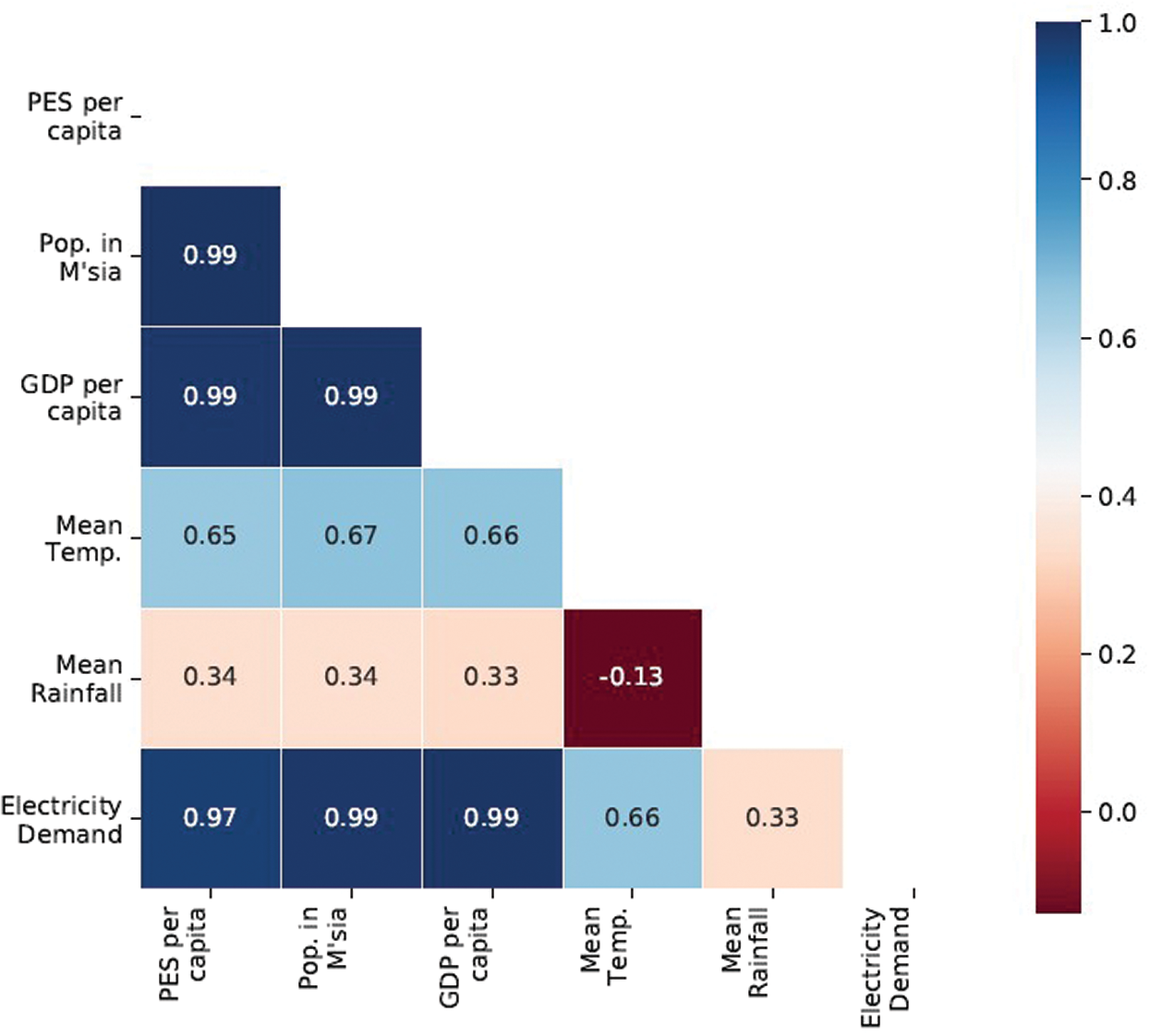
Figure 1: Pearson correlation between variables of the dataset

The historical data of PES, GDP, population, and electricity demand form years 1980 to 2016 were taken from the Malaysia Energy Information Hub database (https://meih.st.gov.my). The data were split into training and validation sets by 7:3 ratio to construct SARIMA models. The models were then used to forecast their respected future values with 95% confidence intervals (CI), from 2017 to 2030. The historical data and the SARIMA results for GDP per capita, population, and PES per capita are as shown in Figs. 2–4, respectively.

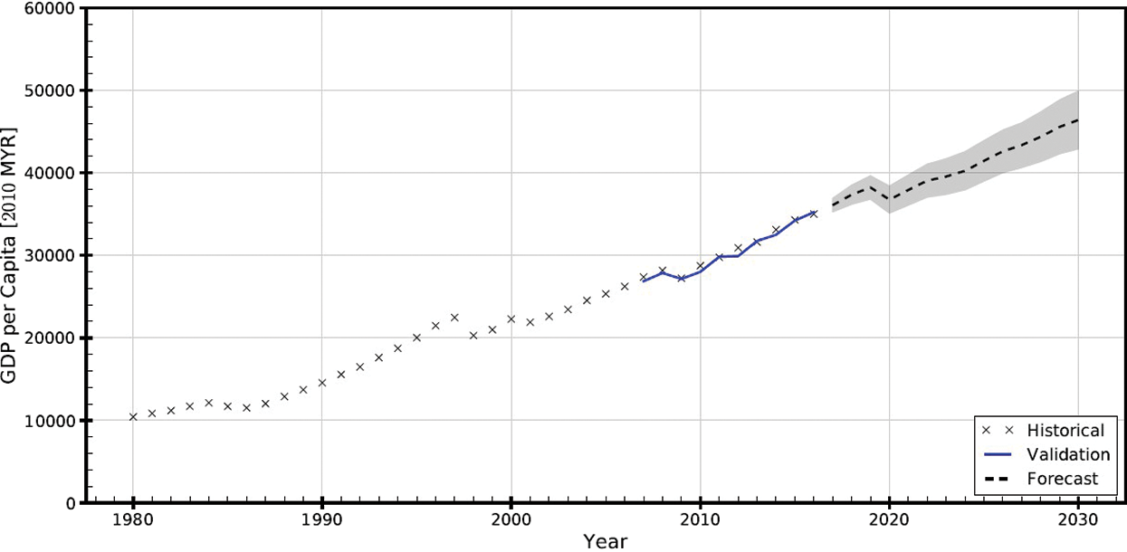
Figure 2: Plot of GDP per capita at constant 2010 MYR value from years 1980 to 2030. The hyperparameters are (0, 1, 0) × (1, 1, 0, 11)

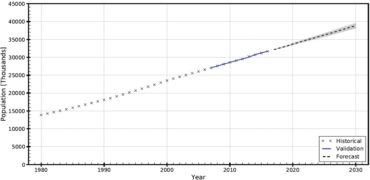
Figure 3: Plot of population in Malaysia from years 1980 to 2030. The hyperparameters are (1, 1, 1) × (0, 1, 1, 7)

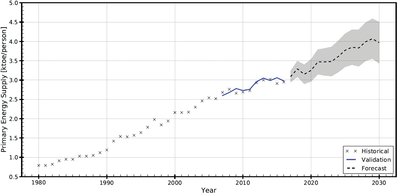
Figure 4: Plot of PES per capita in Malaysia from years 1980 to 2030. The hyperparameters are (0, 1, 0) × (0, 1, 0, 21)

Climate is also a major contributor to energy consumption [17–19]. Only the bi-annual mean average temperature and rainfall data have been taken into consideration in this study. The monthly climate data from 1980 to 2015 used in this study were taken from the World Bank database (http://sdwebx.worldbank.org). As rainfall is weakly correlated to energy demand, only temperature data has been used to construct its SARIMA model. The model was then used to forecast quarterly temperature from 2016 to 2030, as shown in Fig. 5. The statistics of the model residuals presented in Fig. 6 confirmed that the SARIMA model is reliable. Presented in Fig. 7 is the historical and forecast trends of annual mean temperature and rainfall in Malaysia from 1980 to 2030.

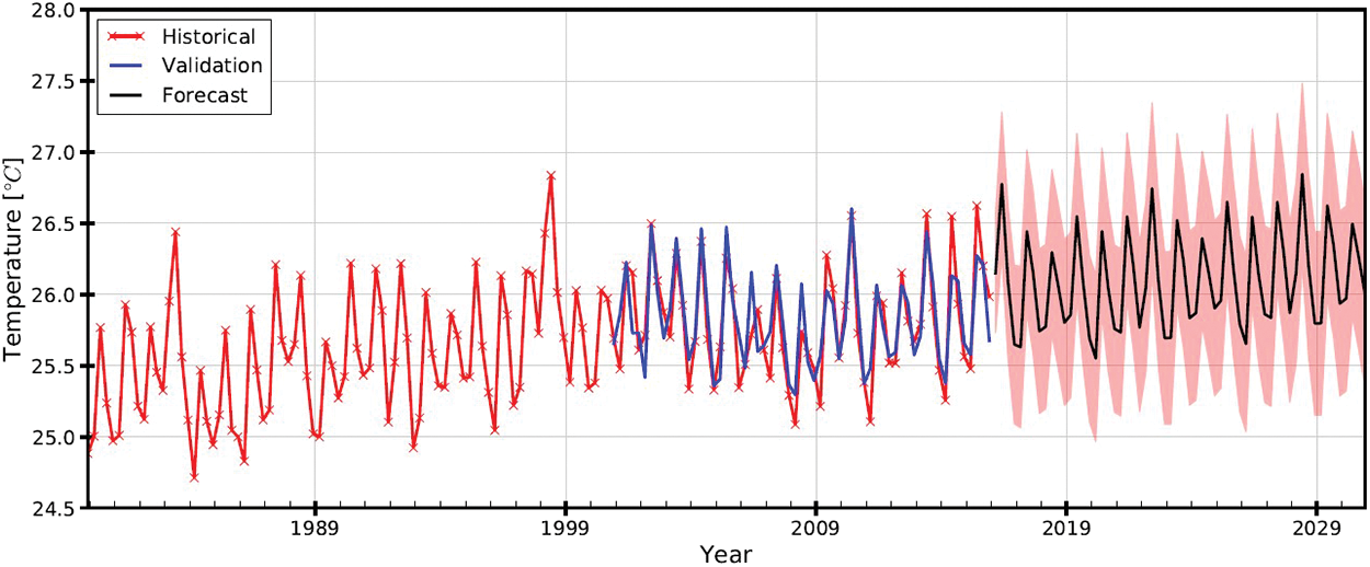
Figure 5: Plot of quarterly mean temperature of Malaysia from years 1980 to 2030. The hyperparameters are (1, 1, 1) × (0, 1, 1, 24)

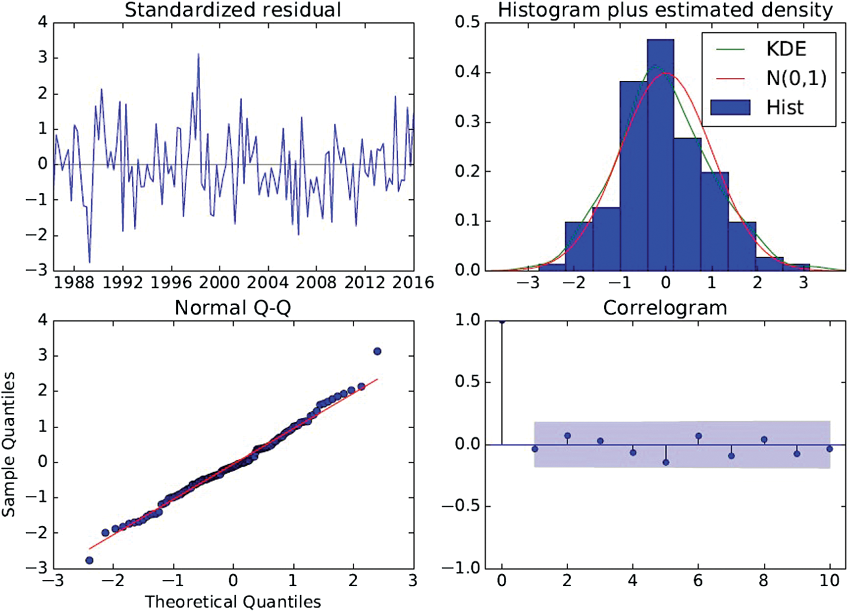
Figure 6: Diagnostic plot quarterly mean temperature of Malaysia

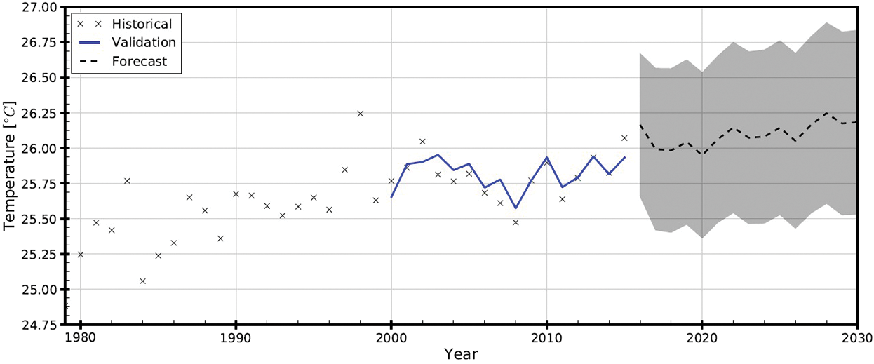
Figure 7: Plot of annually averaged temperature of Malaysia from years 1980 to 2030. The forecast values are based on the SARIMA model presented in Figs. 5 and 6

The forecast values of each variable (see Figs. 2–5, and 7) are described in statistical sense at 95% prediction interval and the variable at each time-step is assumed to be normally distributed and independent. Note that the auto-correlation of each variable has already been dealt with in the SARIMA forecasting stage.

To simulate the possible electricity consumption scenarios from 2020 to 2030, the variables were resampled Nd times at each time-step from the joint probability distribution to construct the inputs for use in ANN model in later stage. The statistical properties of each variable (described in mean (µ) and standard error of mean ( σx¯ )) at each time-step of two-year intervals are presented in Tab. 1.

Table 1: Outputs of SARIMA for use as ANN forecast input

4  Artificial Neural Networks

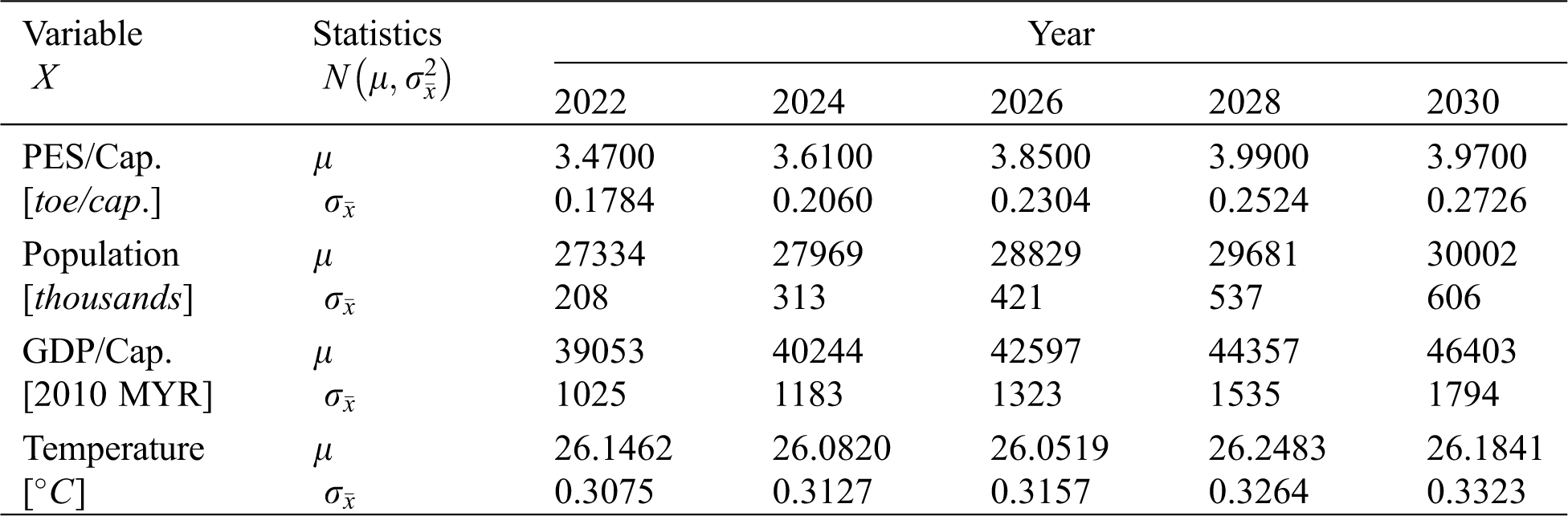
Fig. 8 depicts the Multi-Layer Perceptron (MLP) ANN architecture for this study. It consists of an input layer of four input units, three hidden layers with five units each, and an output layer with one unit for electricity demand. All the units (i.e., neurons) are fully connected in a feed-forward fashion.

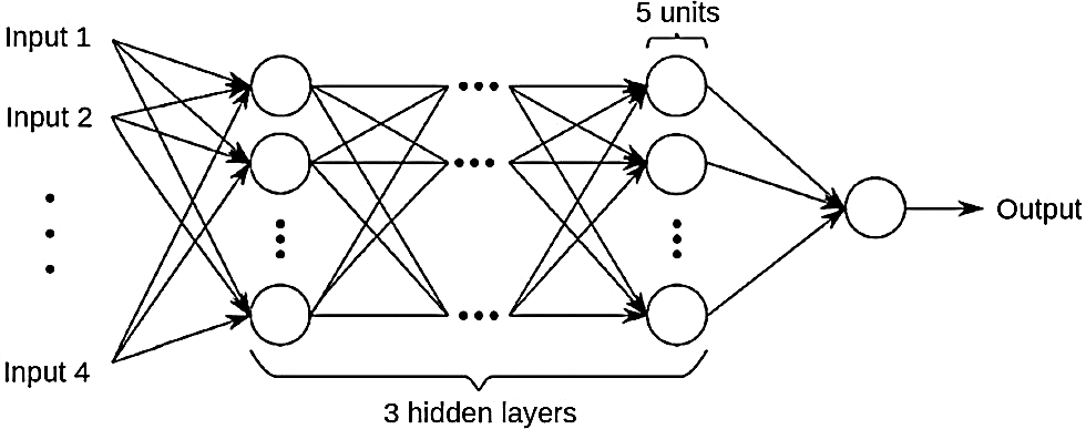
Figure 8: ANN architecture for UQ-SNN

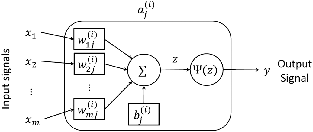
Figure 9: Illustration of perceptron model of neuron aj(i)

Each neuron is modelled as depicted in Fig. 9 known as perceptron. Mathematically, the process of jth neuron in layer ith releases signal y when reacts to input signal {x1,x2,⋅⋅⋅,xm} is as follows:

z=∑km⁡wkj(i)xk+bj(i) (2)

y=Ψ(z)=max(0,z) (3)

where, wkj(i) is the weight assigned to the kth input signal, b is a constant known as bias, and Ψ(⋅) is activation function. In the present study, Rectified Linear Unit (ReLU) activation function has been employed due to its ability to solve vanishing gradient problems and faster in computation [20]. Learning of input-output signals was realised using Back-propagation algorithm. Adaptive Moments (Adam) optimisation [21] has been used to minimise the loss function, ℓ (i.e., the objective function) by iteratively adjusting the weights during the learning phase:

ℓ=1n∑i=1n⁡(Yi−Y^i)2+λ∑j=1m⁡wj2 (4)

The first term of the loss equation is Mean Squared Error (MSE) of the model and targeted outputs for all n number of outputs. The second term of the loss equation is penalty function known as L2-regularization, which consists of a regularisation constant λ for all m number of weights. In conjunction with Back-propagation algorithm, L2-regularization helps to improve the model generalisation by penalising large weight values during the learning phase. In this study, λ=0.001 has been used. On top of that, early stopping is activated when ℓ stopped to improve for 100 successive epochs, such way to prevent overfitting and improve model generalisation.

The historical data of the input variables are split into 7:3 ratio by random for ANN training and testing, respectively. However, the historical data composed of annual data from 1980 to 2015 are not sufficient for ANN to learn the underlying relationships between the input and output variables. To overcome this, the annual data are interpolated to create another 12 data points in between each year, assuming each variable is linear in the respective years.

The modelling is realised with TensorFlow, a Google’s open-source modelling platform for artificial neural network and deep learning [22]. The performance of the ANN is presented in Fig. 10. Both D’Agostino K2 and Shapiro-Wilk tests confirm that the validation error ( ϵm ) is Gaussian. The R2 of the cross-validation plot of computed and validation datasets is 0.9994. A SARIMA model with hyperparameters (0, 1, 2) × (0, 1, 1, 3) has been constructed for validation purposes, with R2 score of 0.9787. This confirms that the proposed ANN can predict better than the conventional SARIMA method. The detail simulation results from both methods are tabulated in Tab. 2.

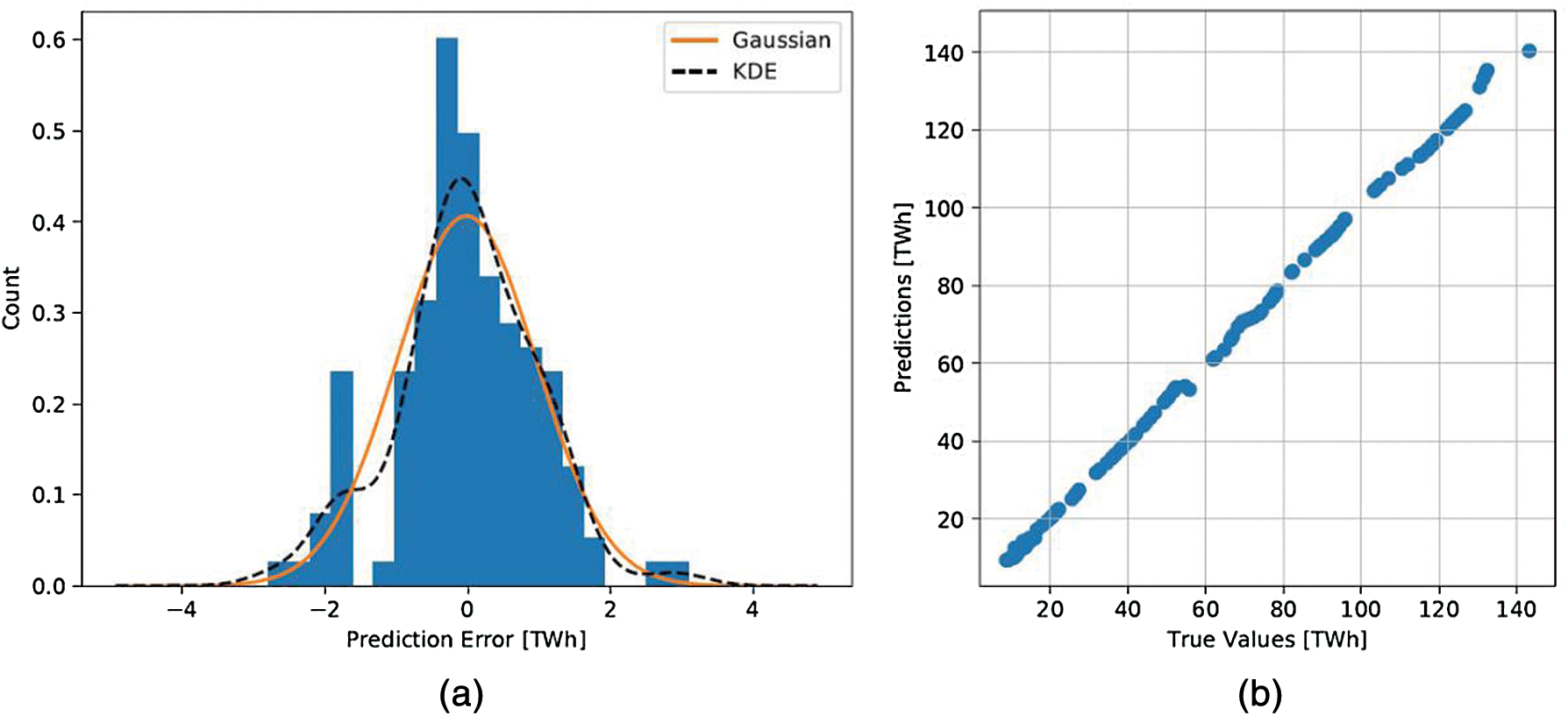
Figure 10: ANN model performance: (a) Validation error; (b) Cross-validation plot

5  Long-Term Electricity Demand Forecasting

Fig. 11 illustrates the UQ-SNN model architecture. The uncertainty of each input variables is described with their respective statistical properties obtained with SARIMA modelling (see Tab. 1). The uncertainty induced by the ANN model, is treated as an input variable using the ϵm obtained in the ANN model validation stage. The final output Y of the model with uncertainty can be described as follows:

Y=f(X1,⋯,X4)+ϵm (5)

where the bold font X and ϵm represent the Nd samples of input and model error with uncertainties. To determine Nd, sample convergence tests have been carried out on the sample µ and σx¯ of X and ϵm . About 10000 samples are required from the multi-dimensional joint probability distribution using Latin-Hypercube Sampling (LHS). Nd samples are drawn at each year of interest and fed into the ANN model to yield Nd size of forecast output. The results are presented in Fig. 12.

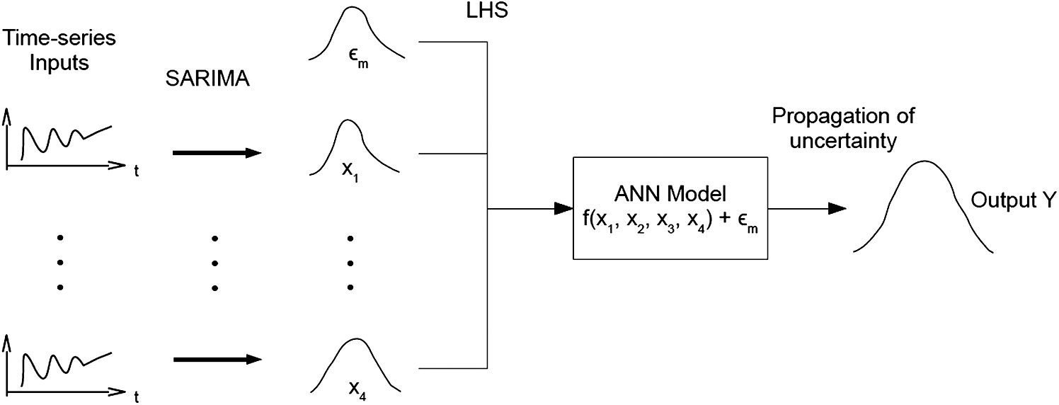
Figure 11: UQ-SNN model architecture

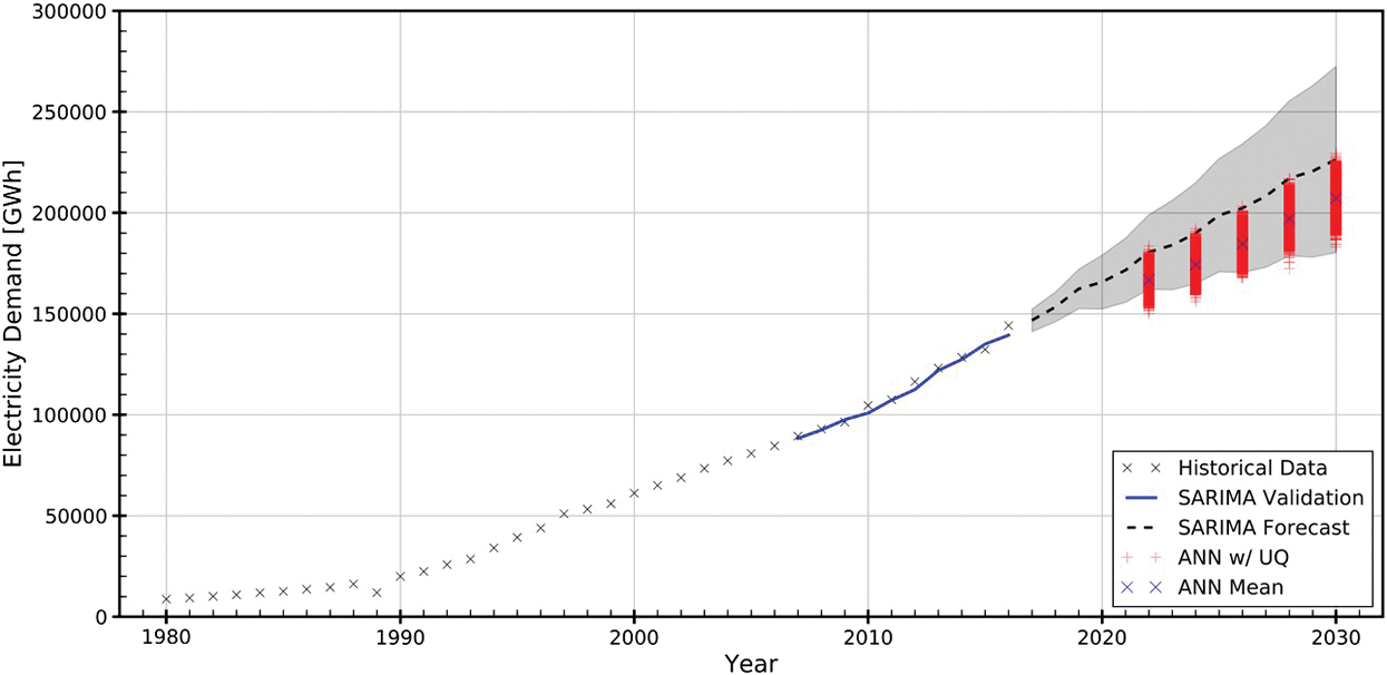
Figure 12: LTLF using SARIMA and UQ-SNN for Malaysia

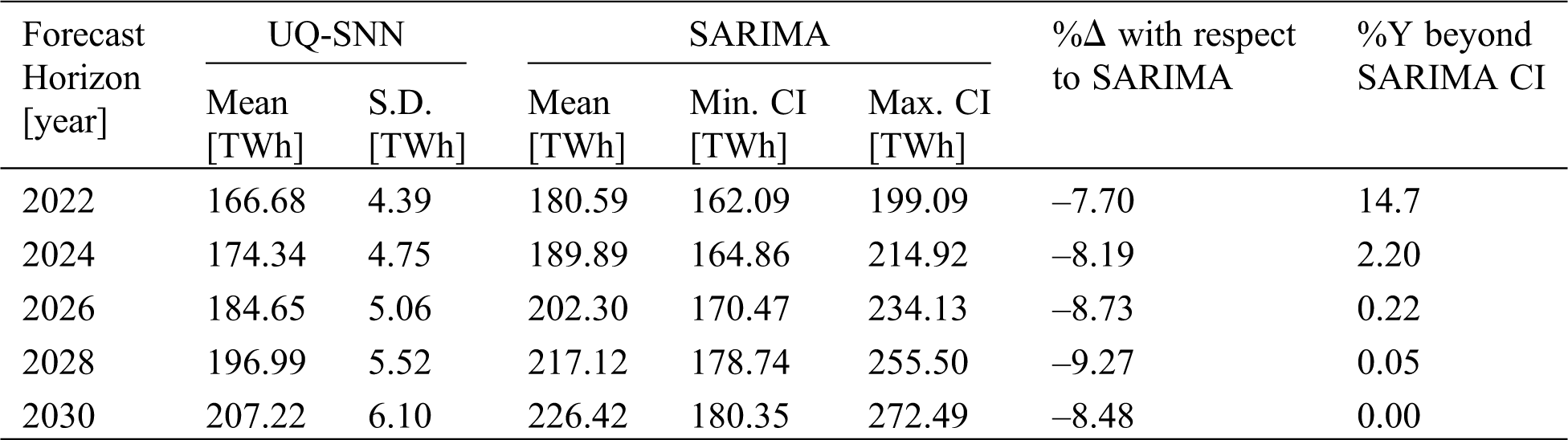
Tab. 2 presents the LTLF results obtained using SARIMA and UQ-SNN, alongside with the comparison of both methods in terms of percentage difference with respect to SARIMA results (%∆) and percentage of UQ-SNN outputs (%Y) that fall outside the SARIMA 95% CI. In general, the UQ-SNN predicts a slower electricity consumption growth than SARIMA. By year 2030, the electricity consumption in Malaysia projected by UQ-SNN is 207.22 TWh, about 8.48% lower than SARIMA prediction. When uncertainty is concerned, all the consumption predicted by UQ-SNN fall inside the SARIMA 95% CI. Although UQ-SNN produces lower consumption growth than SARIMA model, its predicted mean electricity consumption at each year of interest is still within the SARIMA’s 95% CI bounds. Therefore, the results obtained by the UQ-SNN are comparable with the SARIMA model.

Table 2: Comparison of LTLF using SARIMA and UQ-SNN

6  Conclusions

LTLF is crucial for optimum operation and planning of electric power systems. A new LTLF approach called UQ-SNN has been developed and applied to forecast to electricity demands of Malaysia from 2022 to 2030. GDP per capita, PES per capita, population growth, and temperature have been used as inputs for LTLF of Malaysia. Pearson correlation has been used to study the importance of variables involve. Due to limited number of data is available, 12 data points for every year in historical data have been created through interpolation for each of the variables. SARIMA models have been constructed to model the input values with uncertainty of those variables in the forecast horizons.

An MLP ANN model with 3 hidden layers of 5 units each has been constructed for use as forecasting engine in the UQ-SNN framework. Validation error of the ANN using historical data is used to construct the model uncertainty and treated as an input variable. The variables described in uncertainty are then sampled 10000 times using LHS Monte-Carlo simulation to yield the electricity demands in statistical sense. The forecast results are then compared with SARIMA prediction for electricity demands in the forecast horizons. Considering that the mean values of the proposed ANN model are within 10% different than the SARIMA model, it is reasonable to conclude that the proposed method is comparable with the conventional SARIMA model.

The proposed UQ-SNN can capture input and model induced uncertainties, which is crucial in LTLF. Although only 4 variables have been used in this study, the proposed method is flexible and can be easily extended to include other variables to increase the model complexity and accuracy. By 2030, UQ-SNN predicts that Malaysia will consume 207.22 TWh of electricity with SD of 6.10 TWh.

Funding Statement: The project is funded by the Ministry of Higher Education Malaysia, under the Fundamental Research Grant Scheme (FRGS Grant No. FRGS/1/2016/TK07/SEGI/02/1).

Conflicts of Interest: The authors declare that they have no conflicts of interest to report regarding the present study.

This work is licensed under a Creative Commons Attribution 4.0 International License, which permits unrestricted use, distribution, and reproduction in any medium, provided the original work is properly cited.