Energy Engineering

DOI: 10.32604/EE.2021.014627

ARTICLE

Probabilistic Load Flow Calculation of Power System Integrated with Wind Farm Based on Kriging Model

Lu Li1, Yuzhen Fan2, Xinglang Su1,*and Gefei Qiu1

1Faculty of Land Resource Engineering, Kunming University of Science and Technology, Kunming, 650500, China
2School of Control and Computer Engineering, North China Electric Power University, Beijing, 102206, China
*Corresponding Author: Xinglang Su. Email: ednali@126.com
Received: 13 October 2020; Accepted: 29 October 2020

1  Introduction

With the large-scale integration of renewable energy sources such as wind power and photovoltaics (PV) into the grid, there are more and more random factors in the operation of power system, which intensifies the uncertainty of system operation [1]. The calculation of probabilistic load flow (PLF) can take into account the influence of random disturbance or uncertain factors in the operation of power system on steady state operation of system, comprehensively evaluate the weak points and potential risks in the operation of system, and provide valuable information for planning and scheduling department to make decisions, which has always been a focus of research [2,3].

The common calculation methods of PLF include simulation methods and analytical methods. In simulation methods, Monte Carlo simulation (MCS) method [4] owns high accuracy when the sampling scale is large enough, but it takes a long time, so it is usually used as a standard method to evaluate the accuracy of other PLF methods. In analytical methods, convolution method performs convolution calculation according to the probability distribution function of input random variable and obtains the probability distribution characteristics of output random variable [5], which concept is clear but calculation burden is large. In order to solve the above problems, an approximate method is introduced, that is, on the premise of not reducing the accuracy, a mathematical model with a small amount of calculation and a calculation result similar to the actual simulation result is constructed to replace the actual simulation program. Moreover, common approximate models include polynomial response surface method (RSM) [6], artificial neural network (ANN) model [7], and support vector machine (SVM) function model [8], etc. However, polynomial response surface model has a lower fitting degree for nonlinear problems; the characteristics of SVM model varies with its used functions; ANN model is a “black box” model, which lacks strict statistical test and is easy to fall into local extremum. Kriging model is a kind of smallest unbiased variance estimation method estimating the unknown information, which can achieve global approximation in the design space and has high fitting accuracy [9,10].

Both analytical and approximate methods assume that random variables in probabilistic power flows are independent of each other. When it deals with random variables with correlation, new steps are needed to solve the correlation problem of random variables. Haesen et al. [11] used Nataf inverse transformation to predict wind speed to obtain a wind speed series with correlation. Liu et al. [12] transformed multidimensionally correlated non-normal random variables into independent normal random variables based on marginal probability distribution. Bin et al. [13] proposed a simulation method of correlated random variables based on Copula theory and rank correlation coefficient based on cumulative distribution function of random variables. The above correlation modeling methods all need to know the probability distribution function of random variables, but for non-normal multi-dimensional random variables, it is difficult to give a complete joint probability distribution [14].

Kriging is a regression algorithm for spatial modeling and prediction (interpolation) of stochastic process based on covariance function. This paper proposes a combined Kriging model and polynomial normal transformation (PNT) method to calculate PLF of wind farm access to system. Firstly, PNT is used for wind speed prediction to obtain wind speed sequences related to wind turbine clusters, while output model of wind turbine cluster is established. This method does not need to know the probability distribution function of input random variable, but only needs to use polynomial normal transformation according to its digital characteristics to quickly and accurately obtain relevant wind speed sequences. Then, taking the output of PNT as input, relationship between system response and random input is established by Kriging model, thus probability statistics of system response can be calculated. Finally, a wind farm in Yunnan power grid is taken as an example to verify the effectiveness, accuracy, and rapidity of the proposed method.

2  Polynomial Normal Transformation

In this paper, PNT is adopted to transform the non-normally correlated multi-dimensional random variables into the normal uncorrelated variable space, take sampling points in the normally uncorrelated variable space, and then inversely transform these sampling points to the original non-correlated variable space. This transformation-inverse transformation process enables the method to deal with the PLF problem with correlated random variables [15,16].

Common polynomial normal transformation methods mainly include third-order polynomial normal transformation (TPNT) [17], fifth-order polynomial normal transformation (FPNT) [18] and ninth-order polynomial normal transformation (NPNT) [19]. Considering the calculation accuracy and complexity of polynomial normal transformation, this paper employs the most widely applied third-order polynomial normal transformation (TPNT).

Assume a set of correlated multidimensional random variables, denoted X=[x1,x2,⋯,xm]T , where the mean value and standard deviation of xi is μxi and σxi , and the correlation coefficient matrix of these variables is expressed by

RX=[1ρx1,x2ρx2,x11⋯ρx1,xm⋯ρx2,xm⋮⋮ρxm,x1ρxm,x2⋮⋯1] (1)

where ρxi,xj represents the correlation coefficient between xi and xj .

Besides, xi can be expressed as a third-order polynomial of a standard normal distribution vector, i.e.,

xi=a0,i+a1,izi+a2,izi2+a3,izi3 (2)

where a0,i , a1,i , a2,i , and a3,i denote polynomial coefficients.

The polynomial coefficient can be obtained from the probabilistic weighted moment (PWM) of random variable. Suppose PWM of random variable xi is βiγ , and its unbiased estimation [20] can be expressed as

βiγ=1n∑k=γ+1n(k−1)(k−2)⋯(k−γ)(n−1)(n−2)⋯(n−γ)xik (3)

The linear moment of xi can be obtained from PWM of the variable, as follows [21]

{λ1,i=β0,iλ2,i=2β1,i−β0,iλ3,i=6β2,i−6β1,i+β0,iλ4,i=20β3,i−30β2,i+12β1,i−β0,i (4)

The coefficient of the polynomial can be obtained according to the linear moment of xi , as follows

{a0,i=λ1,i−1.81379937λ3,ia1,i=2.25518617λ2,i−3.93740250λ4,ia2,i=1.81379937λ3,ia3,i=−0.19309293λ2,i+1.574961λ4,i (5)

The above transformation transforms non-normal random variables into normal random variables. In order to ensure that the correlated coefficient matrix of random variables remains unchanged in the transformation process, correlated coefficient matrix RZ between variables that obey normal distribution needs to be further given by

RZ=[1ρz1,z2ρz2,z11⋯ρz1,zn⋯ρz2,zn⋮⋮ρzn,z1ρzn,z2⋮⋯1] (6)

The detailed relationship between RX and RZ can be referenced in literature [22], as follows

6a3,ia3,jρzi,zj3+2a3,ia3,jρzi,zj2+(a1,i+3a3,i)(a1,j+3a3,j)ρzi,zj+[(a0,i+a2,i)(a0,j+a2,j)−ρxi,xjσxiσxj−μxiμxj]=0 (7)

where ρzi,zj is the correlated coefficient between zi and zj ; σxi and σxj denote the standard deviation of xi and xj , respectively; μxi and μxj mean the expected value of xi and xj , respectively.

Solve the above unary cubic equation and select the root that satisfies −1≤ρzi,zj≤1 , ρxi,xjρzi,zj≥0 as the value of ρzi,zj .

At this time, Z is still correlated, so it needs to be transformed into an independent normal distribution by using orthogonal transformation, as follows

Z=LU (8)

where the lower triangular matrix L is the Cholesky decomposition of correlation coefficient matrix RZ : RZ=LLT ; U=[u1,u2,⋯,un]T is a random variable subject to independent normal distribution.

Substitute Eq. (8) into Eq. (2), the original space X can be obtained. The calculation process of TPNT prediction of wind farm groups related to wind speed can be referred to Appendix A.

3  Kriging Model Method

3.1 Modelling of Kriging

Kriging model was proposed by Krige, a South African geologist, in 1951, which was first applied to geostatistics. Subsequently, Sack et al. [23] applied it to engineering design, and Remero et al. [24] applied it to structural reliability analysis in 2004. Since then, the application field of Kriging model has been explored and studied continuously.

As an approximate model, the essence of Kriging model instead of actual simulation program is to approximate the relationship between system response and design variables with Kriging model, which is composed of a parametric model and a non-parametric model. It is more flexible than the simple parametric model and simultaneously overcomes the limitation of non-parametric model in processing high-dimensional data [25]. Kriging model simulates a certain point with the help of known information around this point, so it establishes a model related to known information, which requires few parameters to be determined, small calculation amount, and simple model. In addition, the estimation model can be determined through a small number of sample tests.

Kriging model assumes that the actual relationship between system response and random variables can be expressed as

y(x)=fT(x)β+z(x) (9)

where β denotes the regression coefficient; f(x) is the regression model; z(x) is a random process, which obeys the normal distribution N(0,σ2) , but the covariance is non-zero. The covariance of z(x) can be expressed as follows

cov[z(xi),z(zj)]=σ2R(θ;xi,xj) (10)

where R(θ;xi,xj) is the correlation function between sample points xi and xj ; θ is the relevant parameter.

The commonly used regression models and related functions are listed in Appendices B and C respectively. Research shows that the type of regression model does not play a decisive role in the accuracy of simulation [26]. In order to simplify the calculation process, the regression value f(x) is set as 1. The existence of z(x) is the fundamental reason why Kriging model is different from the response surface, and it plays a decisive role in simulation accuracy of model. In this paper, Gaussian correlation equation [27] is employed as

(θk;xi,xj)=exp(−∑k=1nN⁡θk(xki−xkj)2) (11)

where nN denotes the number of random variables; xki and xkj are the k th components of xi and xj ; θk means the correlated parameter.

After the regression model and correlation function are determined, the expression of approximate response y^(x) of y(x) concerning point x to be measured can be established. The known training sample is denoted as S=[x1,x2,⋯,xm]T , its actual response value is Y=[y1,y2,⋯,ym]T , and m is the capacity of training sample. Then the estimated value of any point x to be measured is

y^(xnew)=f(xnew)Tβ^+r(xnew)R−1(Y−Fβ^) (12)

where f(xnew) is the regression quantity; R is a symmetric matrix consisting of R(θk;xi,xj) with a diagonal element of 1 and a size of m×m ; F is the regression matrix F=[f(x1),f(x2),⋯,f(xm)]T ; r(xnew) is the correlation vector between measured point and sample point, which can be expressed as

r(xnew)=[R(θ;xnew,x1),R(θ;xnew,x2),⋯,R(θ;xnew,xm)] (13)

The maximum probability estimation factor is expressed as

β^=(FTR−1F)−1FTR−1Y (14)

The correlated model needs to solve the relevant parameter θ , and according to the maximum probability estimation, it can be obtained as

σ^2=1m(Y−Fβ^)R−1(Y−Fβ^) (15)

The relevant parameter θ is determined by solving an optimization problem as follows

maxθ>0−mln⁡(σ^2)+ln⁡(detR)2 (16)

At this point, Kriging model is established.

3.2 Case Studies of Kriging Models

The numerical example of Eq. (17) is used to verify the simulation effect of Kriging model. In the sampling space, four groups of training sample points with scales of 15, 25, 35, and 45 are respectively taken, which are substituted into Eq. (17) to obtain four sets of response values, and Kriging model is constructed. Zhu et al. [28] proposes a method to solve Kriging model, in which two main functions are dacefit and predictor. The function dacefit establishes Kriging model based on sample points, while the function Predictor calculates the response value of the measured points based on Kriging model.

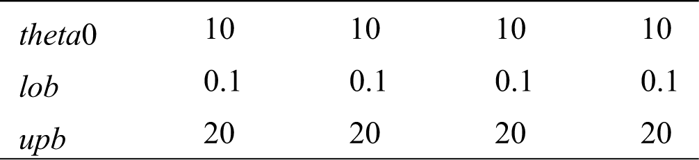
When constructing Kriging model, it is necessary to give the initial value theta0 of the relevant function parameter θ in Eq. (13), and the lower limit lob and upper limit upb of the search range, and their length is equal to the number of design variables. The initial value and search range of θ in this example are shown in Tab. 1.

{y1=x12+x22−x3x4y2=2x12−x22+x32−x4−1≤xi≤1,i=1,2,3,4 (17)

Table 1: The parameter settings of Kriging model

After the model is established, the accuracy of the model should be tested. Randomly generate 100 sets of sample points to be tested in the sampling space, and substitute them into Kriging model and Eq. (17) to obtain the corresponding predicted and actual values. Their relative error is provided in Tab. 2, which shows that the established Kriging model owns good approximate accuracy.

Table 2: The relative error of Kriging model

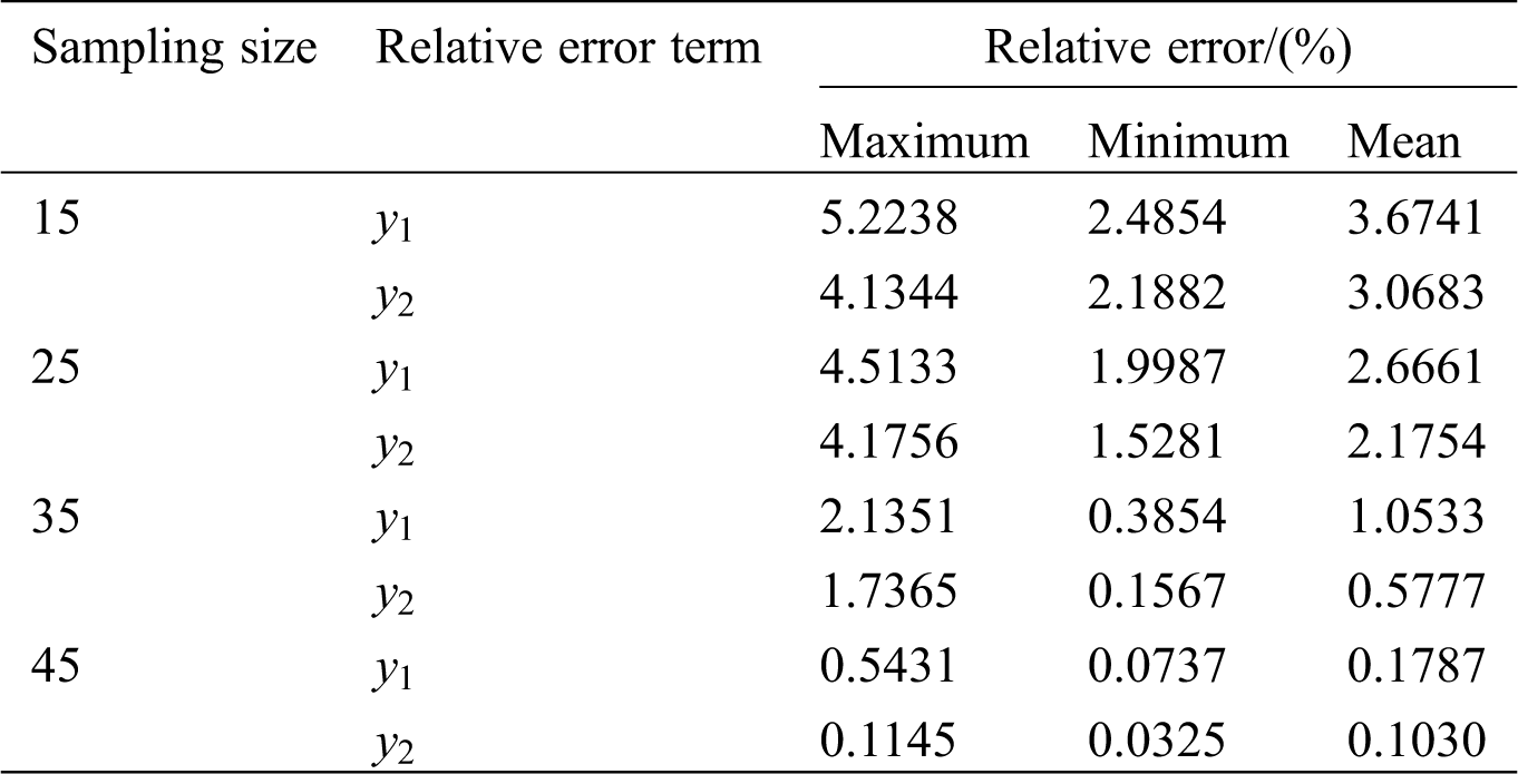
Fig. 1 indicates the mean relative error between the predicted value and the actual value of Kriging model. It can be seen from that the accuracy of Kriging model is related to the size of training sample. The larger the training sample size is, the higher the accuracy of Kriging model will be.

Figure 1: The mean of relative error between predictive value of Kriging model and real value

4  Calculation Steps

In the deterministic power flow calculation, node injection power equation and branch power equation [29] of system can be expressed by

{X=f(W)L=g(X)=g(f(W)) (18)

where W is the power injected into the node; X is the node voltage; L is the branch current; f is the power equation injected into the node; g is the branch power equation.

This paper defines output of wind turbine clusters in the node injected power as input variable and the amplitude of node voltage and the power of branch as output variable. When the input variable is a random variable, the output variable becomes a random variable. PLF problem is to obtain the probability distribution or digital characteristics of output variable when input variable is random.

During calculation, the sample value of output of n groups of wind turbine clusters is firstly generated by TPNT, and then the deterministic power flow is calculated by employing sample value of each group to obtain the corresponding node voltage and branch power of n groups, and then Kriging model is established [30]. Then, TPNT generates output sample values of N groups of wind turbine clusters, and Kriging model is used to obtain the estimated values of node voltage and branch power corresponding to N groups, calculate their probability statistics and compare them with the exact solution based on Monte Carlo method.

The calculation process is shown in Fig. 2 while the basic steps are as follows:

1.    Input basic data: the number of wind turbine clusters m , the training sample size N , the sample size n to be tested;

2.    TPNT method is used to generate a series of wind speed sequences with a scale of n×m and calculate the output of the corresponding wind turbine clusters;

3.    The node voltage and branch power corresponding to N groups are calculated by deterministic power flow calculation, and Kriging model is established;

4.    TPNT method is used to generate a set of wind speed series with a scale of N×m , and the corresponding output of wind turbine clusters are calculated;

5.    The estimated values of node voltage and branch power corresponding to N groups are obtained by Kriging model;

6.    The probability statistics of Kriging model results are calculated and compared with the exact solution based on Monte Carlo method.

Figure 2: Calculation flow chart

5  Case Studies

Based on historical wind speed data of an actual wind farm in Yunnan Power Grid, Kriging model is established, and the power flow calculation is performed on PSD-BPA through command line programming [31]. All case studies are undertaken by Matlab 2019a through a personal computer with IntelRcoreTMi7 CPU at 2.0 GHz and 32 GB of RAM. Monte Carlo method runs 5000 times to obtain near the wind farm node voltage and branch power of statistical information as accurate values, and 50 times in comparison with the results of Kriging model simulation input.

This wind farm has four wind turbine clusters, with installed capacity of 49.5 MW, 42 MW, 34.5 MW, and 42 MW respectively, and total installed capacity of 168 MW, operating with constant power factor of 0.95. Fig. 3 is a regional grid structure diagram of wind farm access system, which is connected to 220 kV main network in the 220 kV area by Node 2 through 110 kV line of two LGJ-300 conductors [32,33].

Figure 3: Structure diagram of regional grid after accessing wind farm

Fig. 4 shows the probability density curve of historical wind speed sequences and TPNT generated wind speed sequences (wind turbine cluster 1 and wind turbine cluster 2 are taken as examples). It can be seen from that wind speed sequences generated by TPNT are very close to the measured historical data, which indicates that TPNT method is effective.

Suppose historical wind speed and parameters of marginal probability distribution function of wind speed generated by TPNT are ηar and ηat , respectively. The relative error index of the parameters of marginal probability distribution function can be expressed by Eq. (19)

ζa=|ηat−ηarηar|×100% (19)

where ηar and ηat are the historical given value of parameter a and the fitting value of TPNT method, respectively.

In order to facilitate the calculation of Eq. (19), probability distribution model of wind speed adopts Weibull distribution that fits well with the actual statistical distribution of wind speed [34], and its probability distribution function can be expressed as

f(v)=kc(vc)k−1exp(−(vc)k) (20)

where v represents wind speed; k and c are the shape parameters and scale parameters of Weibull distribution, respectively, which can be approximated by the expected value of wind speed μv and standard deviation σv :

k=(σv/μv)−1.086 (21)

c=μvΓ(1+1/k) (22)

where Γ represents the gamma function.

The accuracy of correlation model established by TPNT method can be evaluated through Eq. (19), and calculation results are shown in Tab. 3. It can be seen that the correlation samples generated by TPNT have high accuracy in fitting the parameters of marginal probability distribution function of input random variables, and the sample quality keeps improving with the increase of sampling scale.

Table 3: Relative error index of Weibull distribution parameters of wind speed

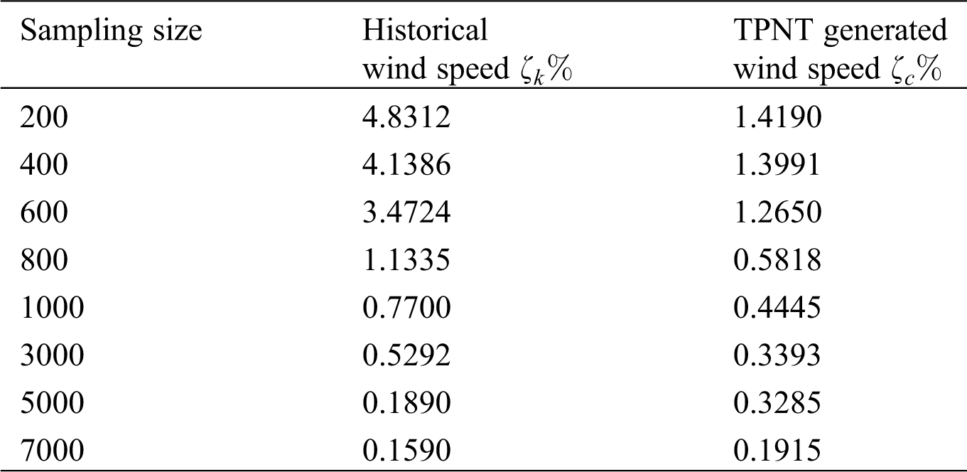
Figure 4: Probability density curves of wind speed. (a) Wind turbine cluster 1, (b) Wind turbine cluster 2

The voltage amplitude of two nodes near wind farm and power of three branches are selected as the observed values, which are numbered as Node 1, Node 2, Branch 1, Branch 2, and Branch 3, respectively, as shown in Fig. 3.

According to the historical wind speed data of 4 wind turbine clusters, a set of relevant wind speed sequences are generated from TPNT to establish wind turbine cluster output model, which is connected to the system for 50 basic power flow calculations to obtain the corresponding 50 voltage groups of Nodes 1 and 2, along with the response values of active power of Branch 1, Branch 2 and Branch 3. Kriging model is constructed according to 50 groups of response values, and 5000 groups of node voltage and branch power are generated by the constructed Kriging model, and the statistical results of 5000 Monte Carlo simulations are compared and analyzed to verify the validity, accuracy, and rapidity of Kriging model.

In Fig. 5, the probability density distribution curve of the voltage amplitude of Node 1 and Node 2 are obtained by Kriging model, and compared with the simulation result based on Monte Carlo method. As can be seen from Fig. 5, the results of 50 times Kriging model method have a high degree of fitting with 5000 times MCS, indicating that Kriging model can well simulate system output.

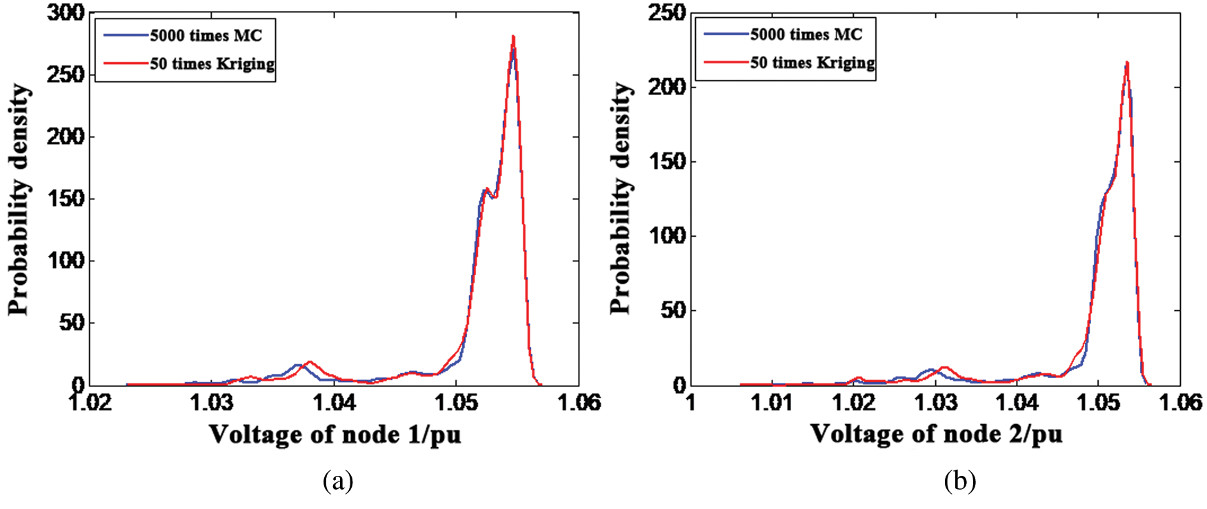
Figure 5: Probability density curves of the related bus voltages under Kriging and recorded history datum. (a) Node 1, (b) Node 2

Fig. 6 compares the probability density distribution of active power of three branches obtained by two methods. The probability density curve obtained by Kriging model fits the histogram obtained by MCS well.

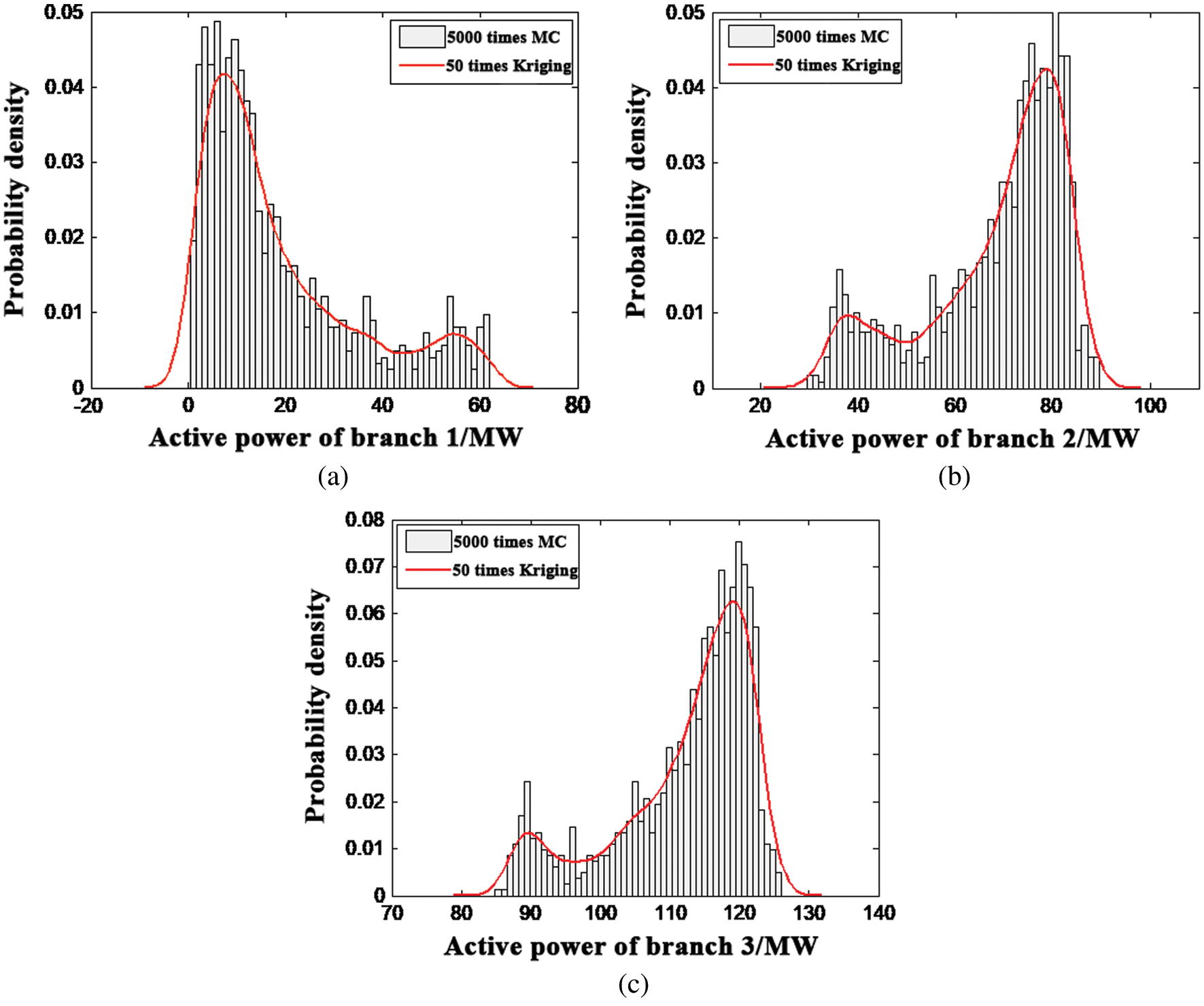
Figure 6: Probability density distribution of the related branches’ power flow under Kriging and recorded history datum. (a) Branch 1, (b) Branch 2, (c) Branch 3

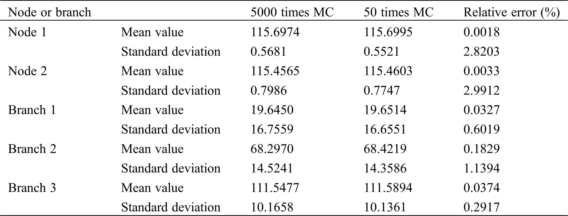
Table 4: Branch powers and bus voltage expectations and standard deviations

Let the simulation results of Kriging model and Monte Carlo method be ξmc and ξkrig , respectively, and the relative error between them is:

ε=|ξmc−ξkrig|ξmc×100% (23)

Tab. 4 compares mean value and standard deviation of the grid related node voltage and branch power. It can be seen from that the mean value and standard deviation of the Kriging model results and the relative error between the exact value are below “0.2%” and “3%”, respectively, which once again verifies the high accuracy of Kriging model.

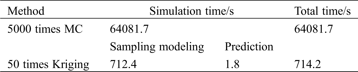
Tab. 5 shows the simulation time of two methods. It shows that simulation time of Kriging model method is far less than that of Monte Carlo method, which proves the rapidity of the method proposed in this paper, and solves the problems of the traditional random analysis method with many simulation times and long simulation time.

Table 5: Simulation time of the two methods

6  Conclusions

Due to the proximity of geographical locations in the same wind farm, the wind speed between different wind power clusters has a strong correlation, so that the output of each wind turbine cluster has a strong correlation. In this paper, TPNT method is adopted to model wind turbine clusters with relevant wind speed, and Kriging model is applied to PLF analysis of system. An example of a real wind power farm in Yunnan power grid shows that Kriging model owns 100 times less than MC computation burden. Kriging also owns higher simulation accuracy, which verifies the effectiveness, accuracy, and rapidity of this method.

This paper provides an effective modeling and analysis method for studying PLF problem based on correlation. Compared with traditional random analysis method, it has fast calculation speed and less memory, and can quickly calculate system probability statistics with correlated random variables. Besides, based on calculation and analysis of PLF in this paper, Kriging model method could be applied to the Optimal power flow calculation and analysis of power system. The measured data will be used to verify feasibility of the proposed method.

Funding Statement: The authors received no specific funding for this study.

Conflicts of Interest: The authors declare that they have no conflicts of interest to report regarding the present study.

Appendix A. TPNT Generates Correlation Wind Speed Sequence

Using TPNT to generate a wind speed sequence with a specified correlation coefficient, which mainly includes three parts:

1.    Sampling points are selected from the independent standard normal space U ;

2.    The transformation Z=LU is used to convert these sampling points from space U to space Z ;

3.    Eq (2) is used to transform the sampling point from space Z to the original space X .

The flow chart of TPNT to predict relevant wind speed of wind farm group is depicted in Fig. A1:

Figure A1: Forecasting related wind speed of wind farm group by TPNT method

Appendix B. Regression Model

The regression part of Kriging model simulates the overall trend of the response, which provides global approximations within the design space, commonly employing zero-order, first-order and second-order polynomials, as follows

zero-order, p=1 ,

f1(x)=1

first-order, p=n+1 ,

f(x)=1,f(x)=x,…,f(x)=x

second-order, p=12(n+1)(n+2) ,

f1(x)=1

f2(x)=x1,…,fn+1(x)=xn

fn+2(x)=x12,…,f2n+1(x)=x1xn

f2n+2(x)=x22,…,f3n(x)=x2xn

⋯⋯fp(x)=xn2

Researches indicate that regression part has little effect on the accuracy of the model, and usually just simply takes constant.

Appendix C. Correlation Model

The existence of random function Z(x) is the fundamental reason why Kriging model is different from the response surface, and it plays a decisive role in the accuracy of the model. Z(x) obeys Gaussian distribution N(0,σ2) , but its covariance is non-zero. It is determined by correlation function R(θ;xi,xj) , which is adopted to calculate the degree of correlation between two samples, and can be expressed as follows

R(θ;xi,xj)=∏k=1n⁡Rk(θk;dk)

where dk=xki−xkj .

The common correlation functions are shown in Tab. C1.

Table C1: Correlation function

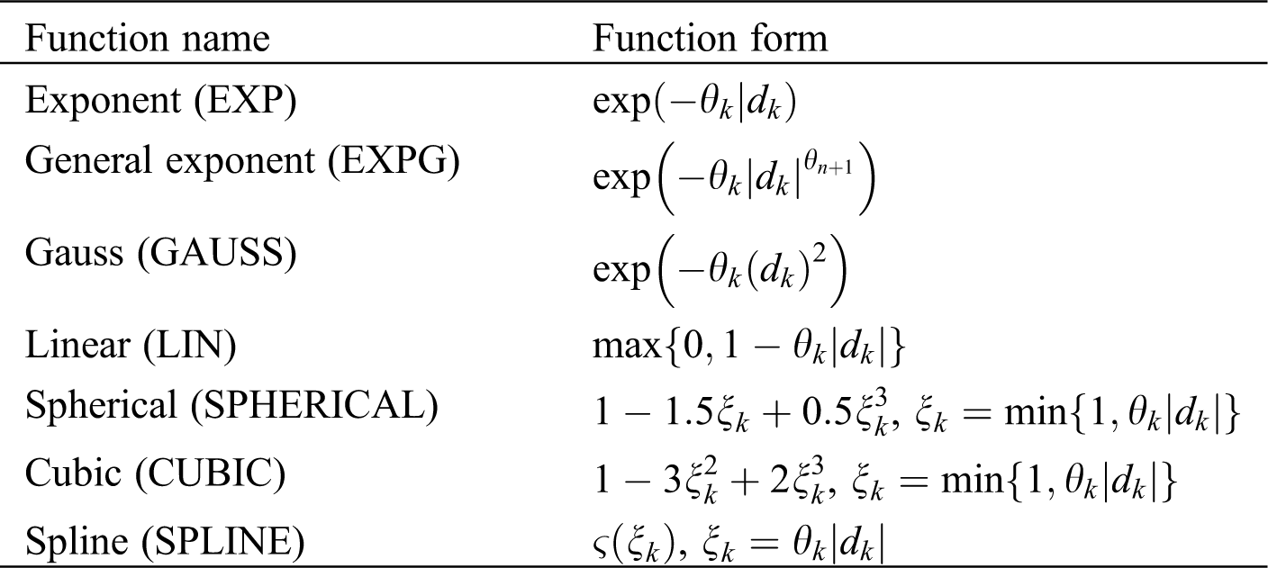
Note: ς(ξk)={1−15ξk2+30ξk30≤ξk≤21.25(1−ξk)30.2<ξk<10ξk≥1

This work is licensed under a Creative Commons Attribution 4.0 International License, which permits unrestricted use, distribution, and reproduction in any medium, provided the original work is properly cited.