Approach for the Simulation of Linear PDEs with Constant Coefficients, Testing Multi-Dimensional Helmholtz and Wave Equations

Nomenclature

1  Introduction

Linear and nonlinear partial differential equations (PDEs) are widespread in scientific and engineering problems. Mathematical models in physics, mechanics, and other fields can be applied to describe the physical phenomena. Many phenomena have been modeled by the linear type PDEs. However, for more complex conditions on the material property and geometric domain, the modeling requires nonlinear type PDEs. An ambitious method recently proposed is the splitting technique to linearize the nonlinear PDEs [1]. At each iterative step, we need to solve the linear PDEs, which are basic requirements in the solutions of PDEs.

For the wave equations, rare analytic solutions are gained. In most cases, we need to numerically solve the wave equations [2–6]. Recently, Chen et al. [7] developed a novel spatial-temporal radial Trefftz collocation method for 3D transient wave propagation analysis.

For the linear PDEs with constant coefficients the typical analytic processes to derive the series solutions are the separation of variables, deriving ordinary differential equations (ODEs) which are in general coefficients varying like the Bessel equation and the Legendre equation, solving the corresponding Sturm-Liouville problem to determine the eigenfunctions and eigenvalues, and finally determining the expanding coefficients to match the specified conditions. In the traditional method, we may encounter difficulty in that the solution bases are some special functions, which are not elementary functions. The analytic process would become tedious when the dimension of the linear PDE is raised. To overcome these difficulties, we will propose a novel method to transform the second-order multi-dimensional linear PDE to a second-order ODE with constant coefficients, which can greatly simplify the analytic works and derive a very powerful method with elementary functions or the compositions of elementary functions as the bases of the series solutions.

We consider a boundary value problem (BVP) for the Helmholtz equation:

(1)

(2)

where or and is a given constant. is a smooth boundary of with and is the outward normal derivative on the surface .

Next, we consider an initial boundary value problem (IBVP) for the wave equation:

(3)

(4)

(5)

(6)

where or and is a given speed of the wave. is a smooth boundary of which is bounded.

For a harmonic wave motion in the steady state, the wave equation can be reduced to the Helmholtz equation, which is also known as the reduced wave equation [8]. Recently, Fu et al. [9] applied the wave theory to the water wave interactions with multiple-bottom-seated-cylinder-array structures and provided the meshless generalized finite difference method for solving them. Owing to the popular applications of the Helmholtz equation in many areas a lot of numerical methods were developed [10–14]. Among the many methods, the singular boundary method is a powerful one to solve various engineering problems as reviewed by Fu et al. [15]. However, for the Helmholtz equation equipped with a large wave number and given in a complex domain, it is still a great challenge to solve it.

The rest of the paper is outlined sequentially. Section 2 devotes to a new approach of the second-order linear PDEs with constant coefficients, by transforming them to a second-order ODE with constant coefficients. The leading term is multiplied by the characteristic form, whose value determines the particular solutions of the PDE. In Section 3, we introduce new variables to transform the 2D and 3D Helmholtz equations to the second-order ODEs and then derive very useful bases in Section 4. The numerical tests of the 2D and 3D Helmholtz equations are carried out in Section 5. The g-analytic function theory for the wave equation is developed in Section 6, where we prove the g-analytic Cauchy-Riemann equations and provide the g-analytic function as the general solution of the wave equation. New projective bases for multi-dimensional wave equations are derived in Section 7. The numerical tests of 2D and 3D wave equations are carried out in Section 8. Finally, the conclusions are coined in Section 9.

2  New Approach of Linear PDEs with Constant Coefficients

We generalize Eqs. (1) and (3) to the d-dimensional second-order linear PDEs with constant coefficients:

(7)

where is a symmetric matrix.

In the characteristic theory of second-order linear PDEs, the characteristic form [8,16].

(8)

is crucial, where with the characteristic vector.

We introduce a new projective variable by

(9)

where we relax to which may be a complex number. w is the projection of the field point x to a nonzero characteristic vector a, and we seek u(x) to be a projective type solution:

(10)

It leads to

(11)

where the prime denotes the differential of with respect to

Theorem 1. For Eq. (7) with and if w is given by Eq. (9) and u is given by Eq. (10) then

(12)

is a projective type solution. Here, satisfies

(13)

where the parameters are selected to rendering and and satisfy

(14)

Proof. It follows from Eqs. (7), (10), and (11) that

(15)

which by Eq. (8) can be recast to Eq. (13). The fundamental solutions of Eq. (13) depend on the eigenvalue in Eq. (14), which is in general a complex eigenvalue with such that

(16)

where D and E are constants. Inserting Eq. (9) for into Eq. (16), we can derive Eq. (12). □

Eq. (7) belongs to the elliptic type PDEs if the characteristic equation possesses no real solutions of a. In the case of and of Eq. (7), Theorem 1 is insufficient since Eq. (13) is reduced to

(17)

from which only the first-order solution can be achieved in view of Therefore we must consider

(18) to seek a in the complex numbers. The elliptic type linear PDE with and can be recast to the canonical form as the standard Laplace equation:

(19)

Lemma 1. For Eq. (19), if w is given by Eq. (9) and u is given by Eq. (10) then the following particular solutions are available:

(20)

where and

(21) where

(22) in which

Proof. For Eq. (19), Eq. (18) reduces to

(23)

There exists no real solution for a, unless the undesired one with Let

(24)

We can take where k is a parameter and By Eq. (23),

(25)

renders the real solutions of other parameters which are located on the sphere with a radius k in the (d − 1)-dimensional space. Such that we have

(26) which is a complex variable. Taking the exponential of w, generates

(27) and the particular solutions in Eq. (20) follow.

On the other hand, we can generate particular solutions by

(28)

where Through some manipulations Eq. (28) leads to the particular solutions in Eq. (21). By cyclically exchanging the independent variables, we can generate many other particular solutions. □

Up to now the discussions of particular solutions of the linear PDE with constant coefficients are somewhat heuristic and formal. To display the advantage of the present approach, we consider a specific PDE:

(29)

By inspection the general solution is

(30)

where a, b, c are constants, and and are differentiable functions.

Let and We can obtain

(31)

Taking and we obtain as a particular solution. If Eq. (31) reduces to

(32)

which leads to a constant and

(33)

If we take and we can obtain

(34)

as a particular solution. By using the Fourier series, we can generate a particular solution where

(35)

This case shows that the new approach can find the general solution of Eq. (29).

These particular solutions involve the parameters, which can be employed as useful bases to expand the solution of the linear PDE with constant coefficients. Below we will give definite linear PDEs of Helmholtz and wave equations, and derive the particular solutions involving parameters as the expanding bases of the solutions.

3  New Projective Solutions of Helmholtz Equations

We first construct a new projective solution of Eq. (1) with To facilitate the proof of the new results, we introduce a projective variable in view of Fig. 1:

(36)

where w signifies the distance of the line on the plane to the original point, and the pair is a unit characteristic vector satisfying

(37) where is a parameter. It follows from Eq. (36) that

(38)

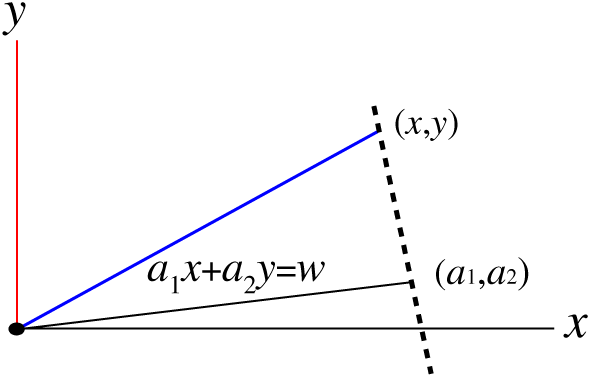
Figure 1: A schematic plot to signify a new projective solution of the 2D Helmholtz equation in terms of w, where w is the projection of to a unit characteristic vector

Theorem 2. For the 2D Helmholtz equation, if w is given by Eq. (36) and Eq. (37) is satisfied, then

(39)

satisfies Eq. (1) with where

(40)

Proof. It follows from Eqs. (39) and (38) that

(41)

Inserting them into Eq. (1) with yields

(42)

If Eq. (37) and the condition (40) are satisfied, then Eq. (1) with is proved. □

We extend the above results to a 3D setting. We introduce the projective variable by

(43)

and the triplet satisfy

(44)

(45)

Theorem 3. For the 3D Helmholtz equation, if w is given by Eq. (43) and Eq. (44) is satisfied, then

(46)

satisfies Eq. (1) with where satisfies Eq. (40).

Proof. It follows from Eqs. (46) and (45) that

(47)

Inserting them into Eq. (1) with yields

(48)

If Eq. (44) and the condition (40) are satisfied, then in Eq. (46) satisfies Eq. (1) with □

4  New Bases for 2D and 3D Helmholtz Equations

Since satisfies Eq. (40), two linearly independent solutions can be derived as follows:

(49)

Correspondingly, for Eq. (1) with we can expand its solution by

(50)

where is the number of undetermined coefficients and and each is given by

(51) which satisfies Eq. (37).

Alternatively, for Eq. (1) with we take

(52)

where

(53) which satisfies Eq. (44).

Up to now, the following innovation points of the paper can be highlighted:

1.    When the linear PDEs encountered are equipped with constant coefficients, the problem of finding a solution is reduced to solving the ODE with constant coefficients.

2.    The problem of finding a solution is thus reduced to solving the characteristic equation, which is a simple algebraic equation for the characteristic vector.

3.    For solving the algebraic equation in the complex domain, all possible bases of the considered PDE can be constructed, without using the technique of special functions.

4.    The solution of the linear PDE is then expanded by the derived bases, which makes it easy to determine the expansion coefficients by the meshless collocation method.

On the other hand, the proposed projective variable method is limited by the following conditions:

1.    The linear PDEs must be constant coefficients, and for the problem with varying coefficients, it is not applicable.

2.    The problem is limited to the continuous one, which with some kind of discontinuity the proposed projective variable method is not applicable.

In the near future, the localization technique as applied in reference [17] may be adopted to the projective variable method for solving the linear PDEs with varying coefficients and with discontinuity.

5  Numerical Experiments of Helmholtz Equations

Now the numerical solutions of the 2D and 3D Helmholtz equations can be carried out by using the projective solutions method (PSM).

We assess the errors of by the maximum error (ME) and root-mean-square-error (RMSE):

(54)

(55)

where denotes the exact solution and the numerical solution, and is the number of tested points.

5.1 Example 1

First, the Dirichlet problem is considered by giving an exact solution:

(56)

which is defined in a square

We take a very large wave number and a referenced value to solve this problem is that the maximum error (ME) = 0.01 is obtained in reference [14]. With m = 100 (n = 200) and collocating points on four sides, we can derive a linear system to determine coefficients and in Eq. (50). Very small errors with and root-mean-square-error are obtained. It is much more accurate than that obtained in reference [14] by using the Trefftz method.

Next, we consider the boundary shape to be a complex amoeba-like curve:

(57)

and we consider the same exact solution (56) with With and we obtain and For the mixed boundary value problem, we can obtain and The high accuracy of the PSM is obvious.

Next, we consider a doubly-connected domain problem with the inner boundary given by Eq. (57) and the outer boundary given by

(58)

Similarly, we take a very large and compare the numerical solution obtained by the PSM to the exact one in Eq. (56). With and collocating points on the boundaries, very small errors are obtained with and

To test the stability of PSM, we add a white noise with an intensity 0.01 on the Dirichlet boundary data. Upon comparing to the noisy error 0.01, quite small errors are obtained with and

To demonstrate that the PSM is a well-posed method, we consider the inverse Cauchy problem on the above doubly-connected domain, where the Dirichlet and Neumann boundary data are imposed on the outer boundary. Upon comparing to the noisy error 0.01, quite small errors are obtained with and For this problem, the resulting linear system is well-posed with 146 steps to obtain the expansion coefficients. If no noise perturbs the Dirichlet and Neumann boundary data, the accuracy is very good with and

5.2 Example 2

Next, the Dirichlet problem is considered for a given exact solution of the 2D Helmholtz equation with

(59)

which is defined in a domain with the boundary:

(60)

With and we obtain and Again the high accuracy of the proposed PSM can be seen.

5.3 Example 3

We consider:

(61)

(62)

where

(63) is the boundary shape of Ω.

Under and the PSM is used to find the solution, which is compared to the exact solutions on where and It is remarkable that when we take very accurate solution with and is obtained. Although for and is obtained. This example shows that the PSM is effective.

Next, we consider a bumpy sphere as the boundary:

(64)

The PSM is compared to the exact solution on of which and are obtained. When we take very accurate solution with and is obtained.

Although is raised to and are obtained, which compared to the maximum value 2.89 is acceptable. When we take very accurate solution with and is obtained.

6  The g-Analytic Function Theory for Wave Equation

The g-analytic function for the one-dimensional wave equation has been derived by Liu [18] based on the g-number theory. In order to derive the g-analytic function for the multi-dimensional wave equation we introduce

(65)

(66)

(67)

where d is a d-dimensional director and ∇ is a d-dimensional gradient operator with respect to x. is a directional derivative of along the direction d.

In terms of we can recast Eq. (3) to

(68)

By Eq. (66), we have

(69)

Summing these equations yields

(70)

due to Thus, from Eqs. (68) and (70), a 2D like wave equation is available:

(71)

Liu [19] has introduced the g number which is the Minkowski space, where 1 and g obey the product rule:

(72)

Using

(73)

we can deduce

(74)

Let

(75)

be the conjugation of w given in Eq. (65). By the chain rule we have

(76)

(77)

(78)

Accordingly, we can derive the following result.

Theorem 4. The d-dimensional wave equation, possesses a general solution where F and G are twice differentiable functions. The function is an g-analytic function if and only if

(79)

Moreover, and satisfy

(80)

by which is an g-analytic function in the -dimensional space-time.

Proof. It is straightforward from Eq. (78) that

(81)

is the general solution of Eq. (3).

Take the operator to the second equation in Eq. (79),

(82)

Take the operator to the first equation in Eq. (79),

(83)

which by Eq. (67) changes to

(84)

Subtracting Eqs. (84) by (82) leads to hence by Eq. (70), we prove the first equation in Eq. (80).

Conversely, the operator acting on the first equation in Eq. (79) generates

(85)

Take the operator to the second equation in Eq. (79),

(86)

which by Eq. (67) changes to

(87)

Subtracting Eqs. (87) by (85) leads to the second equation in Eq. (80). This ends the proof. □

In Theorem 4, Eq. (79) is the g-analytic Cauchy-Riemann equations for the multi-dimensional wave equation, which is appeared in the literature for the first time. As a demonstration of Theorem 4, we take a simple g-analytic function

such that

Using it is easy to verify

Hence, the first g-analytic Cauchy-Riemann equation in Eq. (79) is verified. By

the second g-analytic Cauchy-Riemann equation in Eq. (79) is identified.

Lemma 2. The g-analytic function for the wave equation satisfies

(88)

where and

Proof. In view of Eq. (67) the Cauchy-Riemann equations in Eq. (79) can be written as

(89)

which are sufficient and necessary conditions for to be g-analytic. Inserting into the second one in Eq. (88), leads to

(90)

(91)

(92)

Inserting them into the second one in Eq. (88), yields

(93)

which renders

(94)

Thus, the first one in Eq. (88) is proved. □

Lemma 2 is interesting that any differentiable function is a g-analytic function, where and satisfy the wave equation. The g-analytic function theory bears certain similarities to the analytic function theory for complex functions. The polynomial is a very useful solution of the wave equation, which can generate powerful bases to expand the solution.

Lemma 3. The polynomial is given by reference [20].

(95)

where

(96)

(97)

Proof. The Minkowski length of is

(98)

where we suppose that is a space-like vector with

Thus from Eq. (65), we have

(99)

Let

(100)

and from

(101)

(102)

By Eqs. (99) and (74), we have

(103)

hence the first identity in Eq. (95) is proven by taking the power

By Eq. (98), Eq. (102) can be recast to

(104)

Taking the exponential generates

(105)

which makes

(106)

The powers are given by

(107)

and the combinations of them yield

(108)

We end the proof. The derivation of Eq. (95) is similar to the time-like vector with □

Eq. (95) is a novel polynomial solution of the wave equation. As a demonstration of Lemmas 2 and 3, we consider

such that

It is easy to verify by

and by

7  New Projective Bases for Multi-Dimensional Wave Equations

For the wave equations, we have the following results.

Theorem 5. For the 2D wave equation of Eq. (3) with there exist four types projective solutions:

(109)

(110)

where and is a real number.

Proof. We begin with

(111)

where the pair satisfy

(112)

is a parameter, i.e., i is an imaginary number and is a real number. Hence, is a 2D imaginary vector.

It follows from Eq. (111) that

(113)

Let

(114)

Then, we have

(115)

Inserting them into Eq. (3) with yields

(116)

By Eq. (112), it reduces to

(117)

To satisfy this equation we must take such that

(118)

Any twice differentiable function together with Eqs. (112) and (118) satisfy the wave equation. Because are imaginary numbers, we take

(119)

Then, in view of Eqs. (114), (118), (119), (111) and (112), we can obtain Eqs. (109) and (110) by taking the real and imaginary parts of

(120)

where is a 2D director satisfying □

Theorem 6. For the 3D wave equation of Eq. (3) with there exist four projective solutions:

(121)

(122)

where and is a real number.

Proof. Since the proof is similar to that in Theorem 5, we omit it. □

Eqs. (109) and (110) alone cannot form the bases. Therefore, we generalize them to a series of numbers for for and for by

(123)

Consequently, for Eq. (3) with we can expand the solution by

(124)

where the last two bases are obtained from Lemma 3. The number kc/T is the frequency of the kth-order cosine and sine bases, and T is a given value. For low-frequency waves, we take a large value of T, while for high-frequency waves we take a small value of T.

Alternatively, for Eq. (3) with we can expand the solution by

(125)

where T is a parameter, and

(126)

Remark 1. Let us consider the one-dimensional wave equation in a finite rod with a length L and subject to homogeneous boundary conditions From the Fourier series method the following series solution is known:

(127)

where are the eigenvalues. Indeed, Eq. (127) is a special case of Eq. (124) when it is reduced to one dimension. It is interesting that the present theory can reduce the problem of multi-dimensional wave propagation problem in a finite bounded domain to solve a second-order ordinary differential equation (ODE) with constant coefficients in Eq. (116). The key of this method is the new concept of projection in Eq. (111), where the projective variable w is obtained by projecting to Next, the imaginary wave number vector in Eq. (112) helps us to derive the related series solution. Indeed, the present theory can be deemed as an extension of the Fourier series theory, but without going into the details of the methods of the separation of variables and the determination of eigenfunctions and eigenvalues. The present theory is easily tailored to the problem in an arbitrary domain, which is a main restriction to hinders the application of Fourier series theory.

Remark 2. The present theory is also an extension of the d’Alembert solutions and of the one-dimensional wave equation . Indeed, we can derive

(128)

to be the general solution of Eq. (3) with where is any differentiable function of w as proved in Lemma 2.

8  Numerical Tests of 2D and 3D Wave Equations

Now we are in a good position to test the bases in Eqs. (124) and (125) used in the solutions of 2D and 3D wave equations.

8.1 Example 4

We consider the following exact solution [20,21]:

(129)

and the boundary shape of the 2D domain is given by the following parametric equation:

(130)

(131)

We take collocated points to satisfy the Dirichlet boundary condition and two initial conditions. As suggested by the solution in Eq. (129), we may get rid of the last two bases in Eq. (124). With unknown coefficients are to be determined from a linear system, which is scaled by such that all the column norms equal to [22]. Up to and are obtained, which is quite accurate. However, when we raise to whose results are not so good with and as shown in Fig. 2 by a solid line.

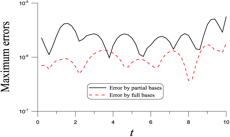
Figure 2: For Example 4 of the 2D wave equation, comparing numerical solutions with partial and full bases for a long-term solution

Therefore, we take the full bases in Eq. (124) into account with and unknown coefficients. For and are more accurate than that using the partial bases. Up to and are obtained, which is quite accurate as shown in Fig. 2 by a dashed line.

To compare with [20], the spatial domain is changed to a unit square. With and and are more accurate than that obtained in reference [20]. ME with respect to t is plotted in Fig. 3.

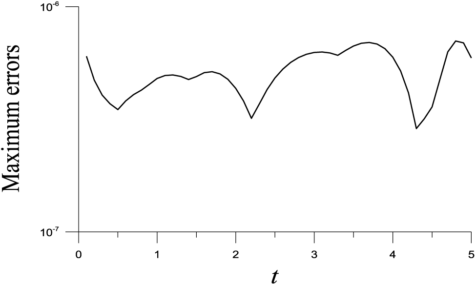
Figure 3: For Example 4 of the 2D wave equation in a unit square, showing maximum errors for a long-term solution

8.2 Example 5

We consider the vibrating problem of a 2D circular membrane with zero boundary condition and zero initial velocity but with the following initial displacement:

(132)

The radius is and The analytical solution is expressed by the Bessel functions:

(133)

where is the zeroth order first kind Bessel function and the first ten eigenvalues are given in the textbook [23].

We take collocated points to satisfy the Dirichlet boundary condition and two initial conditions. With and unknown coefficients to be determined, up to the numerical solution is compared to the one in Eq. (133) with at the point in Fig. 4. They are quite close.

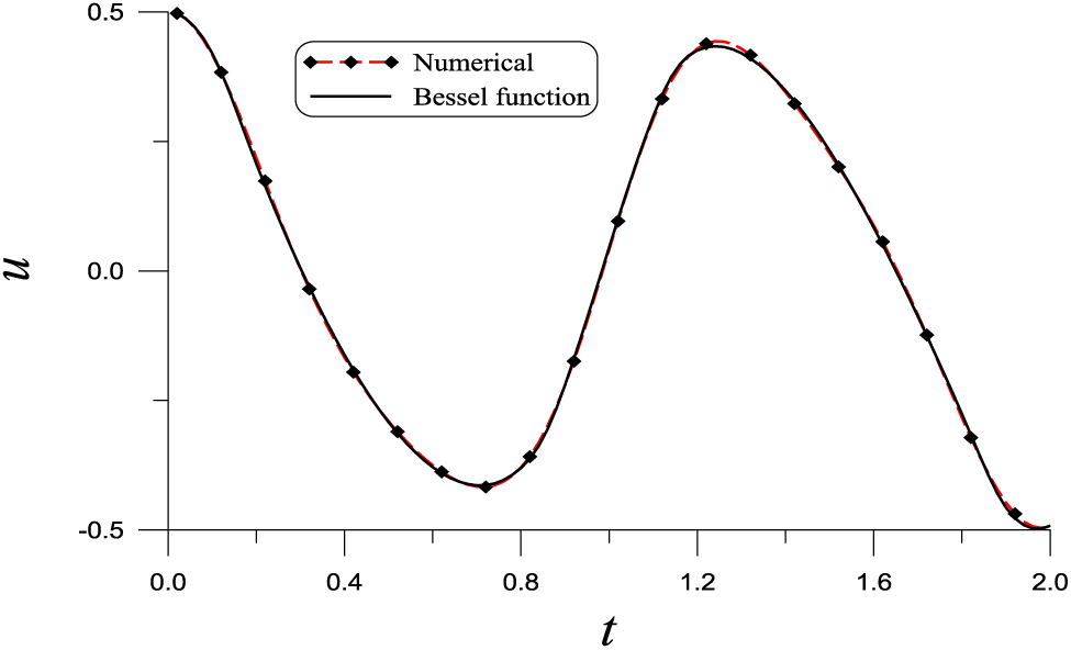
Figure 4: For Example 5 of the 2D wave equation of a vibrating circular membrane, comparing numerical solution with that obtained from the zero-order first kind Bessel function

8.3 Example 6

Consider

(134)

We take collocated points, and with and up to and are obtained. ME with respect to t is plotted in Fig. 5 by a solid line. The numerical solution at and on is with and which is more accurate than that obtained in [20], whose maximum error is

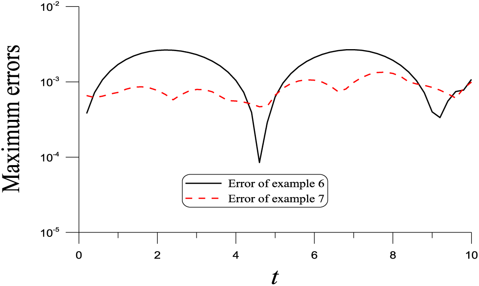
Figure 5: For Examples 6 and 7 of the 3D wave equation showing maximum errors

8.4 Example 7

We give

(135)

We take collocated points, and with and up to and as plotted in Fig. 5 by a dashed line. The numerical solution at and on is with and which is more accurate than that obtained in [20], whose maximum error is

9  Conclusions

Three major topics were treated in the paper to develop the new projective solutions of linear partial differential equations (PDEs) with constant coefficients, 2D and 3D Helmholtz equations, and 2D and 3D wave equations. A new concept of projective variable is introduced, such that we can transform the PDE to the second-order ODEs with constant coefficients, whose leading term is multiplied by the characteristic form. These results are novel and not yet reported in the literature. Depending on the value of the characteristic form we can derive particular solutions involving the parameters, which are used as the useful bases to expand the solutions of linear PDE with constant coefficients. We project the field point to a unit characteristic vector to obtain a new coordinate, which can reduce the 2D and 3D Helmholtz equations to the constant ODE, and then two linearly independent projective solutions involve the unit vector as parameters. The solutions of 2D and 3D Helmholtz equations are easily expanded in terms of these functions as the bases and a powerful numerical technique was created to solve the 2D and 3D Helmholtz equations. We have established the g-analytic function theory for the wave equations. The necessary and sufficient conditions for the g-analytic function were proved to be the g-analytic Cauchy-Riemann equations. The cosine functions, sine functions, and polynomial functions are combined as the bases for the wave equations. Owing to its simple bases, the projective solutions method (PSM) outperforms the conventional methods. Numerical experiments verified the accuracy and efficiency of the PSM for solving the Helmholtz and wave equations.

Acknowledgement: The authors would like to express their great thanks to the reviewers, who supplied good opinions to improve this paper.

Funding Statement: The authors received no specific funding for this study.

Author Contributions: The authors confirm contribution to the paper as follows: study conception and design: Chein-Shan Liu, Chung-Lun Kuo; data collection: Chung-Lun Kuo; analysis and interpretation of results: Chein-Shan Liu; draft manuscript preparation: Chein-Shan Liu, Chung-Lun Kuo. All authors reviewed the results and approved the final version of the manuscript.

Availability of Data and Materials: Data sharing is not applicable to this article as no new data were created or analyzed in this study.

Conflicts of Interest: The authors declare no conflicts of interest to report regarding the present study.

References

1. Liu, C. S., Chang, C. W. (2023). Nonlinear Cauchy/Robin inverse problems solved by an optimal splitting-linearizing method. International Journal of Heat and Mass Transfer, 213, 124329. https://doi.org/10.1016/j.ijheatmasstransfer.2023.124329 [Google Scholar] [CrossRef]

2. Young, D. L., Ruan, J. W. (2005). Method of fundamental solutions for scattering problems of electromagnetic waves. Computer Modeling in Engineering & Sciences, 7, 223–232. [Google Scholar]

3. Shu, C., Wu, W. X., Wang, C. M. (2005). Analysis of metallic waveguides by using least square-based finite difference method. Computers, Materials & Continua, 2, 189–200. [Google Scholar]

4. Godinho, L., Tadeu, A., Amado Mendes, P. (2007). Wave propagation around thin structures using the MFS. Computers, Materials & Continua, 5, 117–128. [Google Scholar]

5. Young, D. L., Gu, M. H., Fan, C. M. (2009). The time-marching method of fundamental solutions for wave equations. Engineering Analysis with Boundary Elements, 33, 1411–1425. https://doi.org/10.1016/j.enganabound.2009.05.008 [Google Scholar] [CrossRef]

6. Gu, M. H., Young, D. L., Fan, C. M. (2009). The method of fundamental solutions for one-dimensional wave equations. Computers, Materials & Continua, 11, 185–208. [Google Scholar]

7. Chen, L., Xu, W., Fu, Z. (2022). A novel spatial-temporal radial Trefftz collocation method for 3D transient wave propagation analysis with specified sound source excitation. Mathematics, 10, 897. https://doi.org/10.3390/math10060897 [Google Scholar] [CrossRef]

8. Chester, C. R. (1970). Techniques in partial differential equations. New York: McGraw-Hill. [Google Scholar]

9. Fu, Z. J., Xie, Z. Y., Ji, S. Y., Tsai, C. C., Li, A. L. (2020). Meshless generalized finite difference method for water wave interactions with multiple-bottom-seated-cylinder-array structures. Ocean Engineering, 195, 106736. https://doi.org/10.1016/j.oceaneng.2019.106736 [Google Scholar] [CrossRef]

10. Fan, C. M., Young, D. L., Chiu, C. L. (2009). Method of fundamental solutions with external source for the eigenfrequencies of waveguides. Journal of Marine Science and Technology, 17, 164–172. https://doi.org/10.51400/2709-6998.1953 [Google Scholar] [CrossRef]

11. Chen, K., Harris, P. J. (2001). Efficient preconditioners for iterative solution of the boundary element equations for the three-dimensional Helmholtz equation. Applied Numerical Mathematics, 36, 475–489. https://doi.org/10.1016/S0168-9274(00)00021-0 [Google Scholar] [CrossRef]

12. Singer, I., Turkel, E. (1998). High-order finite difference methods for the Helmholtz equation. Computer Methods in Applied Mechanics and Engineering, 163, 343–358. https://doi.org/10.1016/S0045-7825(98)00023-1 [Google Scholar] [CrossRef]

13. Chen, W. (2002). Meshfree boundary particle method applied to Helmholtz problems. Engineering Analysis with Boundary Elements, 26, 577–581. https://doi.org/10.1016/S0955-7997(02)00028-0 [Google Scholar] [CrossRef]

14. Kuo, C. L., Yeih, W., Liu, C. S., Chang, J. R. (2015). Solving Helmholtz equation with high wave number and ill-posed inverse problem using the multiple scales Trefftz collocation method. Engineering Analysis with Boundary Elements, 61, 145–152. https://doi.org/10.1016/j.enganabound.2015.07.015 [Google Scholar] [CrossRef]

15. Fu, Z. J., Xi, Q., Gu, Y., Li, J., Qu, W. et al. (2023). Singular boundary method: A review and computer implementation aspects. Engineering Analysis with Boundary Elements, 147, 231–266. https://doi.org/10.1016/j.enganabound.2022.12.004 [Google Scholar] [CrossRef]

16. Zauderer, E. (2011). Partial differential equations of applied mathematics, 3rd edition. New York: John Wiley & Sons. [Google Scholar]

17. Fu, Z. J., Tang, Z. C., Xi, Q., Liu, Q. G., Gu, Y. et al. (2022). Localized collocation schemes and their applications. Acta Mechanica Sinica, 38, 422167. https://doi.org/10.1007/s10409-022-22167-x [Google Scholar] [CrossRef]

18. Liu, C. S. (2015). The g-analytic function theory and wave equation. Journal of Mathematics Research, 7(3), 85–98. https://doi.org/10.1557/JMR.1992.0085 [Google Scholar] [CrossRef]

19. Liu, C. S. (2000). A Jordan algebra and dynamic system with associator as vector field. International Journal of Non-Linear Mechanics, 35, 421–429. https://doi.org/10.1016/S0020-7462(99)00027-X [Google Scholar] [CrossRef]

20. Liu, C. S., Kuo, C. L. (2016). A multiple-direction Trefftz method for solving the multi-dimensional wave equation in an arbitrary spatial domain. Journal Computational Physics, 321, 39–54. https://doi.org/10.1016/j.jcp.2016.05.030 [Google Scholar] [CrossRef]

21. Gu, M. H., Fan, C. M., Young, D. L. (2011). The method of fundamental solutions for the multi-dimensional wave equations. Journal of Marine Science and Technology, 19, 586–596. [Google Scholar]

22. Liu, C. S. (2012). An equilibrated method of fundamental solutions to choose the best source points for the Laplace equation. Engineering Analysis with Boundary Elements, 36, 1235–1245. https://doi.org/10.1016/j.enganabound.2012.03.001 [Google Scholar] [CrossRef]

23. Kreyszig, E. (2006). Advanced engineering mathematics. New York: John Wiley & Sons. [Google Scholar]