 Submit a Paper
 Propose a Special lssue
 Open Access
ARTICLE

Supervised Learning for Finite Element Analysis of Holes under Biaxial Load
School of Mechanical and Aerospace Engineering, Nanyang Technological University, 639798, Singapore
* Corresponding Author: Wai Tuck Chow. Email:
(This article belongs to the Special Issue: Advances in Methods of Computational Modeling in Engineering Sciences, a Special Issue in Memory of Professor Satya Atluri)
Digital Engineering and Digital Twin 2024, 2, 103-130. https://doi.org/10.32604/dedt.2024.044545
Received 02 August 2023; Accepted 07 March 2024; Issue published 06 May 2024
 View Full Text
 Download PDF
Abstract
This paper presents a novel approach to using supervised learning with a shallow neural network to increase the efficiency of the finite element analysis of holes under biaxial load. With this approach, the number of elements in the finite element analysis can be reduced while maintaining good accuracy. The neural network will be used to predict the maximum stress for holes of different configurations such as holes in a finite-width plate (2D), multiple holes (2D), staggered holes (2D), and holes in an infinite plate (3D). The predictions are based on their respective coarse mesh with only 2 elements along the whole quarter perimeter. The result shows the prediction errors are under 5% for all the listed hole configurations. In contrast, the conventional FEM with the respective coarse mesh has errors above 20%. To achieve similar accuracy, the conventional FEM would require finer mesh with at least 6 elements along the perimeter. Furthermore, this setup is also effective in predicting the maximum stress for the 3D problem. With the aid of supervised learning, the FEM analysis of a coarse mesh with only 2 elements along the quarter perimeter can attain prediction errors of less than 2%. For the same coarse mesh, the conventional FEM has errors above 35%. To achieve similar accuracy for the 3D problem, the conventional FEM would require finer mesh with more than 8 elements along the perimeter. This result shows that supervised learning has great potential to enhance the efficiency of finite element analysis with fewer elements while attaining satisfactory results.Keywords
The use of finite element analysis (FEA) to solve problems of engineering is popular in many engineering industries due to its ability to represent complex geometry and capture local stress concentration effects. Furthermore, due to the increasing computational power available and the decreasing costs of FEA software, the use of FEA has grown significantly over the years. Yet, modeling a large segment of a component can still require high computational costs. To keep the computational costs practical, coarser mesh and linear elements are often used. As a result, the accuracy of the model is poor, and it is insufficient for fatigue analysis to be carried out. To achieve the accuracy needed, the sub-modeling of the FEA model is performed in high-stress areas. Sub-modeling is the process of creating a solid model of the local geometry at the region of interest within the global model. Subsequently, the local solid model must undergo mesh refinement together with a transfer of boundary conditions from the global model. Unfortunately, sub-modeling is usually performed manually. Therefore, sub-modeling often is a labor-intensive process especially when the part has many features that require many sub-models. As a result, performing these complex 3-D design iterations with local geometry changes or topology optimizations often requires significant time and resources. Moreover, even with sub-modeling, the choice of 3D elements is often linear due to computational limitations. Hence, a huge amount of effort and resources can be saved if machine learning techniques could be applied to increase the accuracy of the finite element analysis of coarse 3D mesh and reduce the need for sub-modeling.
Machine learning is the usage of models to learn from data and make assessments without being explicitly programmed. The goal is to create a trained neural network model based on the pattern of the training data and be able to make predictions involving different sets of data with similar patterns. Improvement in machine learning techniques over the years has made it an effective tool to be used across many different industries such as finance, social research, and medicine. Improvements can be categorized into two areas, software and hardware. For instance, the algorithm using the Scaled Conjugate Gradient (SCG) is a more robust variant of the original conjugate gradient method (CG). It is less computationally complex and faster. SCG is used as a backpropagation algorithm to minimize errors in the neural network. Moller [1] demonstrated that SCG can converge to a minimum point where the CG cannot due to the Hessian matrix for global error function not being positive definite. In addition, SCG does not include any user-dependent parameters that are crucial for the success of the algorithm, unlike CG. Furthermore, he showed that the calculation complexity of one iteration of SCG can be more than 3 times less than that of the CG method. Meanwhile, the Levenberg-Marquardt method (LM) is developed to solve non-linear least squares problems. Gavin et al. [2–4] demonstrated that LM is more robust than the Gauss-Newton algorithm in minimization tasks where it can converge to the solution even when the starting point is very far off from the minimum. At the same time, it also converges to the minimum point faster than the gradient descent method. Finally, regularization techniques have been developed to curb the problem of overfitting the neural network (NN) to training data sets. One such method is the Bayesian Regularization (BR). Kayri [5] demonstrated that the BR algorithm with tangent sigmoid transfer function in the framework of a single hidden layer feed-forward neural network is effective in predicting nonlinear relations and non-continuous data such as social data. He also showed that using 2 neurons in such a framework has the highest reliability and robustness.
As for hardware advancements, neural processing units (NPU) are increasingly adopted for machine learning tasks which are traditionally performed by the central processing unit (CPU) or graphics processing units (GPU). NPUs are dedicated processing units optimized for power and area efficiency for matrix math. For instance, the 700 MHz NPU used by Google, known as a Tensor Processing Unit (TPU) has a matrix multiplication unit with over 65,000 arithmetic logic units and can process 92 trillion 8-bit operations per second [6]. In addition, Norman et al. [6] expected that rapid improvements will be made in NPU due to its design simplicity. Hence, with the rapid advancement in machine learning algorithms and NPU hardware, there seems to be a huge potential in integrating machine learning with finite element analysis.
Hashash et al. [7] utilized neural network to define the non-linear material constitutive models in the FEA analysis. Manevitz et al. [8] used neural network time series methodology to determine the location for finite element mesh refinement at optimum interval. Chow [9] demonstrated that by using supervised learning algorithms, the errors of coarse mesh can be significantly reduced for holes on a finite-width plate under a uniaxial load. However, more study is required to evaluate if supervised learning can be effectively applied to a more diverse set of problems.
The main objective of this paper is to provide the optimal approach to effectively utilize supervised learning to optimize the FEA of holes under biaxial load in a diverse set of problems. This study also evaluates the extent of reduction in errors by using supervised learning. In this paper, SCG, LM, and BR algorithms were used to train the NN. In addition, pure linear and tangent sigmoid transfer functions will be evaluated. The displacement nodal solutions of the nearest 6 nodes to the quarter-hole’s edge were used as the training parameters. The input data set used to train the NN will consist of a small set of 20 different course mesh of a hole in an infinite-width plate. There will only be 2 elements along the quarter-hole perimeter in the coarse mesh. An analytical solution of a hole under biaxial load will be used as the output target data. Subsequently, the NN will be used to predict the maximum stress of holes under a more diverse range of problems such as holes on a finite-width plate, multiple holes, staggered holes, and holes on the 3D plate.
An artificial neural network consists of neurons, weights, and biases. Using an iterative minimization procedure based on the different back-propagation techniques, the weights are adjusted to reduce the error [10,11]. In addition to weights, biases are included in a neural network to introduce flexibility and better generalization to the neural network. Bias is an extra input to neurons that may allow the neuron to be activated even when inputs are 0. The inclusion of biases is essential in neural networks to prevent overfitting to the training data set [12,13].
Many studies have been done to optimize the weight initializations to curb problems of vanishing gradients and exploding gradients [14,15]. These problems could cause weight updates that are overly small or large which stops the backpropagation from working effectively. However, they are only prevalent in multi-layered neural networks or recurrent neural networks with gradient-based propagation methods. Fortunately, this study uses only one hidden layer in a feed-forward neural network. Hence weight initialization will not be focused on mitigating these problems.
Weight initialization will instead be focused on reducing training time. The Nguyen-Widrow algorithm will be used to initialize the weights and biases for all 3 backpropagation methods. This eliminates most of the weight adjustments, hence only small adjustments are needed to be made during training. The Nguyen-Widrow algorithm has been demonstrated to be able to accelerate the training process and testing accuracy [16–19]. Since the Nguyen-Widrow method requires the layer’s transfer function to have a finite input range, it will only be used when the layer has a tangent sigmoid transfer function. For layers with a pure linear transfer function, weights and biases will be initialized randomly with values between −1 and 1.
The following three sections present the three different back-propagation algorithms used in the study. These three backpropagation methods were chosen as they are the most common methods used in MATLAB machine learning.
2.1 Scaled Conjugate Gradient (SCG)
The Conjugate Gradient (CG) method is implemented as an iterative algorithm in the minimization problem. It can be regarded as being between the gradient descent algorithm and Newton’s method. The gradient descent algorithm requires the calculation of first order derivative which is the gradient to find the minimum of the cost function. It has a slow convergence rate where subsequent steps often contradict previous steps. On the other hand, Newton’s method requires the calculation of second order derivative which has high computational cost. CG method accelerates the convergence rate of the steepest descent by performing the search along conjugate directions such that subsequent steps never contradict previous steps. It also has lower computational costs compared to Newton’s method. The Scaled Conjugate Gradient (SCG) method which is faster and more robust will be used [1].
Consider a quadratic function:
where
The algorithm is started by choosing the initial weight vector
The weight vector and residual are then updated:
The direction vector of the next step,
such that
CG method will fail and converge to nonstationary point if matrix
where
Similar to SCG, the Levenberg-Marquardt (LM) method is an iterative process such that the final weight is obtained through iterations with step
Consider the cost function:
where
where
where
The minimum point of the cost function has a gradient of 0. By taking the derivative of
Eq. (11) is known as Gauss-Newton update. By introducing a damping factor
where
2.3 Bayesian Regularization (BR)
To reduce overfitting, this method uses regularization parameters
When
The application of Bayesian Regularization (BR) within the framework of the LM algorithm will be used [27]. At each iteration, one step of the LM algorithm will be used to minimize
This section will first present the analytical stresses and displacement of a hole in an infinite-width plate under uniaxial load. Next, it will introduce the approach to how the analytical solution can be integrated with supervised learning for both uniaxial load and biaxial load.
3.1 Stress and Displacement around a Hole under Uniaxial Load
In Fig. 1, a hole in an infinite-width plate is subjected to uniaxial tensile load where the tensile load only exists in one primary axis. The stress field solution under uniaxial load [28] can be integrated to obtain the displacement field as follows:
where
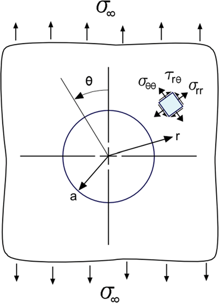
Figure 1: Figure of a hole in an infinite plate under uniaxial tensile load
3.2 Approach to Apply Supervised Training for Uniaxial Load
The input data set used to train the NN will consist of a set of 20 course mesh of a hole in an infinite-width plate. An analytical solution of a hole under biaxial load will be used as the output target data. A coarse mesh of the quarter-hole is shown in Fig. 2. The infinite-width effect is approximated using half width = 20 × hole radius. Ansys 2D linear element, Plane 182 [29], is used. There are only 2 elements along the perimeter of the quarter-hole in the coarse mesh. The displacement nodal solution of the nearest 6 nodes to the quarter-hole’s edge is used as the training parameters. The 6 nodes are shown in Fig. 2. The transfer function of the first layer will be either tangent sigmoid or pure linear, while the transfer function of the output layer will be set to pure linear.
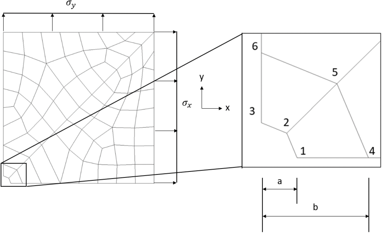
Figure 2: Coarse mesh of a quarter-hole with 2 elements along the perimeter
The material property is based on Aluminum, where
where i is node = 1 to 6 and
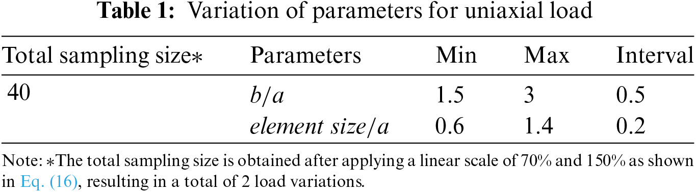
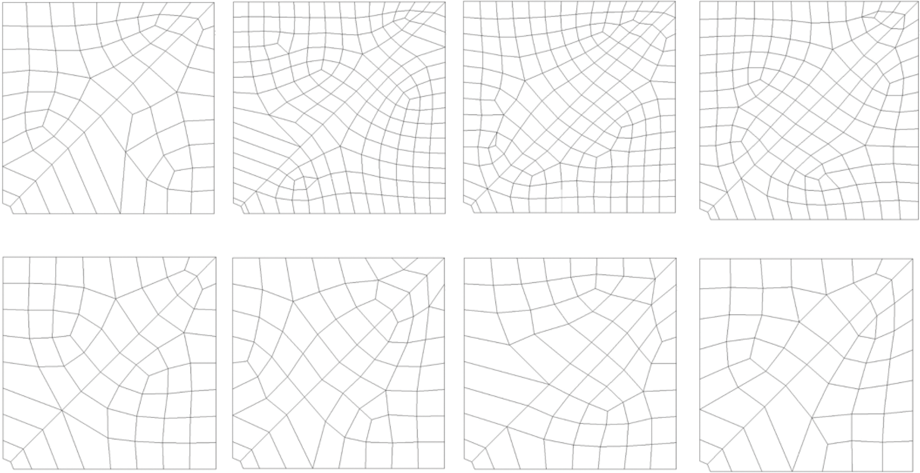
Figure 3: Samples of mesh variations
The neural network consists of a single hidden layer as shown in Fig. 4. The effectiveness of the neural network in predicting the maximum stress of a single hole in a finite-width plate will be investigated using different combinations of training parameters based on the displacements of the 6 nodes shown in Fig. 2. Two approaches to conduct supervised training will be used, one for uniaxial and the other for biaxial load.
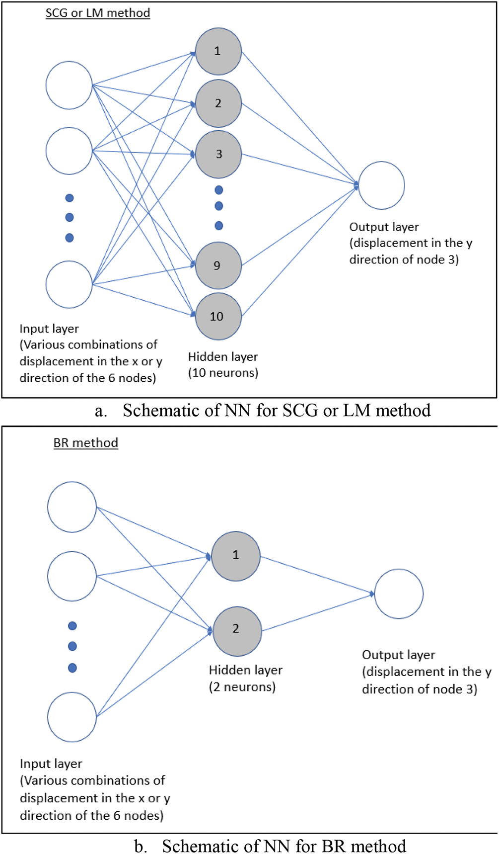
Figure 4: Neural network with 1 output
10 neurons will be used for the SCG and LM method, while 2 neurons will be used for the BR method as the BR method requires fewer neurons to perform effectively as demonstrated by Kayri [5]. Numerical experimental was conducted and the result shows the accuracy improvement starts to taper off as the number of neurons for SCG and LM methods approaches 10. This could be because there are only 10 input parameters from the 6 nodes (2 DOF × 6 nodes with 2 less due to symmetric boundary conditions). The target consists of the analytical solution of only
where i is node = 1 to 6 and
where
3.3 Stress and Displacement around a Hole under Biaxial Load
Since deformation is small, assuming that the response is linear, the principle of superposition can be applied to the uniaxial load solution [28]. In Fig. 5, the analytical stress for hole under applied biaxial stress,
where
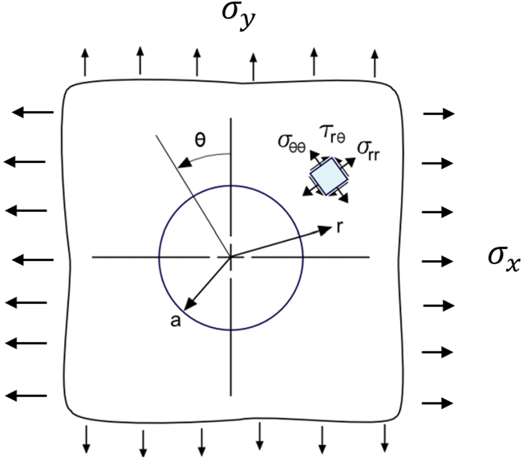
Figure 5: Figure of a hole in an infinite plate under biaxial tensile load
By applying superposition on plane stress displacements under uniaxial load given by Eqs. (14) and (15), the radial and tangential displacement of the hole under biaxial load and plane stress conditions are as follows:
where
Aside from plane stress conditions, this paper also evaluates the effectiveness of a 2D coarse mesh training data set generated under general plane strain conditions. Under general plane strain conditions, the strain in the z-direction
Using Eqs. (19) and (20) to convert the polar stresses in Eqs. (24) and (25) to applied stresses in the cartesian coordinate system, then by integrating the strains, the displacements in terms of applied stresses
Notice that Eq. (26) is a function of the z-component strain
To obtain
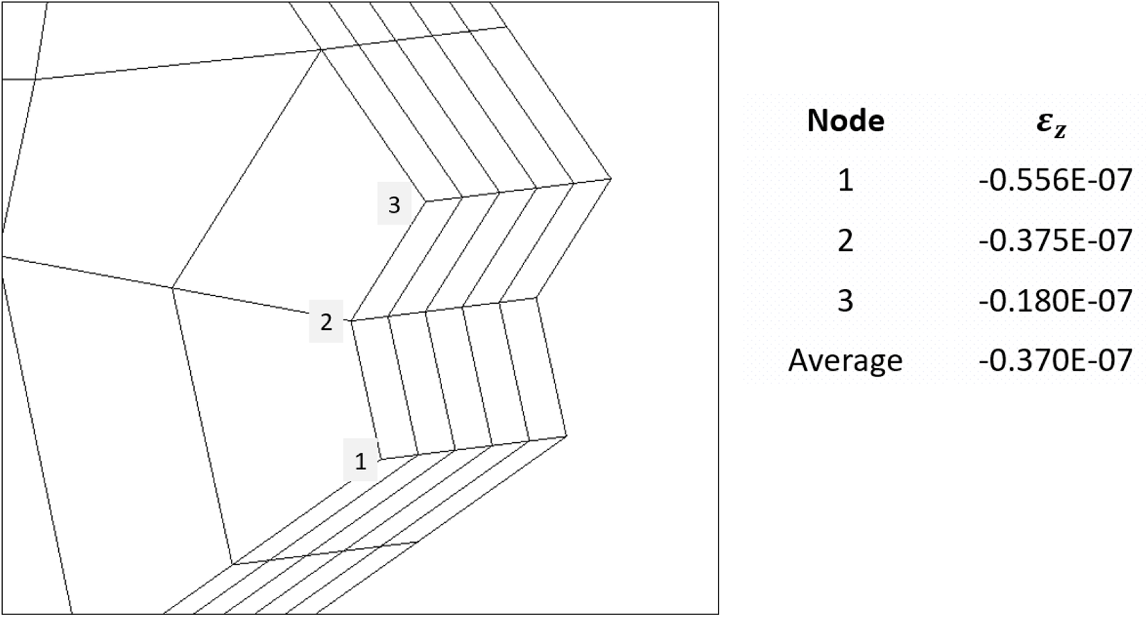
Figure 6:
3.4 Approach to Apply Supervised Training for Biaxial Load
The neural network is trained with the same set of 2D coarse mesh used in the uniaxial load case. Fig. 7 shows the neural network models used for the analysis. In Fig. 2,
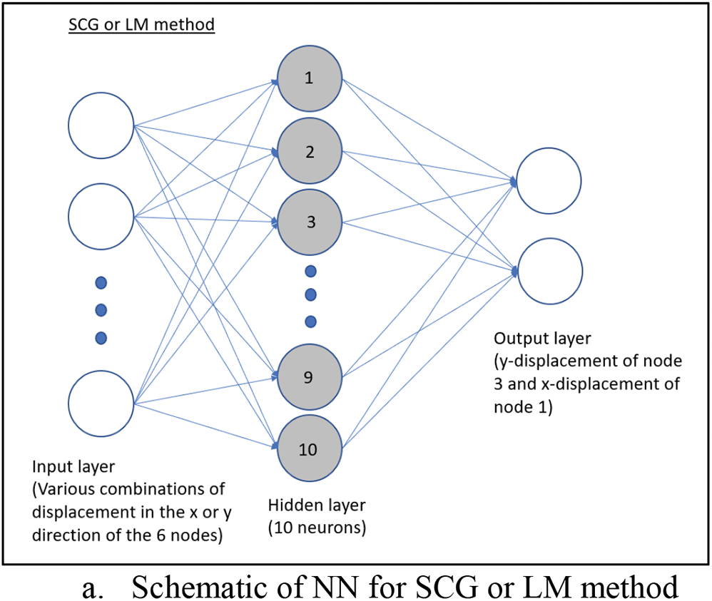

Figure 7: Neural network with 2 outputs
The target data consists of analytical solutions of
where i is node = 1 to 6 and
When substituting
Finally, by using Eq. (20), the predicted maximum stress which is the tangential stress at node 1 can be obtained.
In this study, Matlab’s library [30], fitnet, is used for the neural network supervised training with ‘trainscg’ (SCG), ‘trainbr’ (BR), and ‘trainlm’ (LM) as the backpropagation method. For SCG and LM methods, 70% of the training sample size is used for the training of neural networks, 15% for the validation of the neural network model, and the remaining 15% for the testing of the accuracy of the model. For the BR method, which is a self-validating algorithm, 85% of the training sample size is used for training and 15% for testing. At the hidden layer, either tangent sigmoid or pure linear transfer function will be used. Their effectiveness will be evaluated against each other. In addition, uniaxial and biaxial approaches are compared.
For the prediction of 2D mesh, plane stress condition is used to generate the 2D coarse mesh training data set. For the prediction of 3D mesh, the general plane strain condition is used to generate the 2D coarse mesh training data set [9].
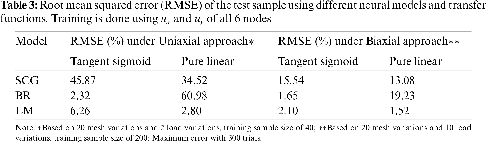
4.1 Infinite-Width Hole: Neural Network Option
The accuracy of the test result based on the displacement at all 6 nodes as training parameters is shown in Table 3. BR method with tangent sigmoid transfer function and LM method with pure linear transfer function offer low prediction errors for both approaches.
To further improve the result, the study evaluates the displace field on the element attached to the maximum stress location at Node 1. In this element, Node 2 and Node 5 have non-zero
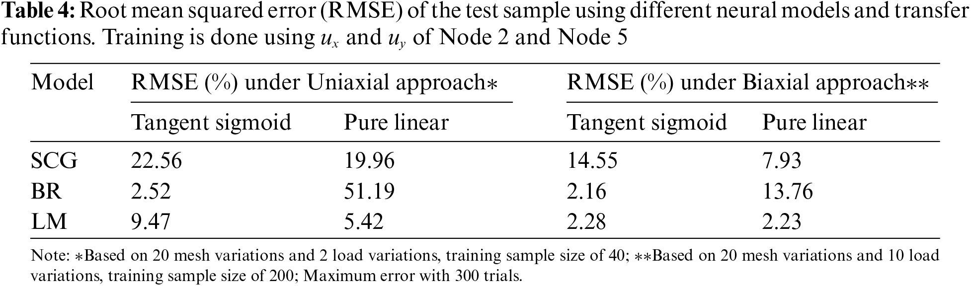
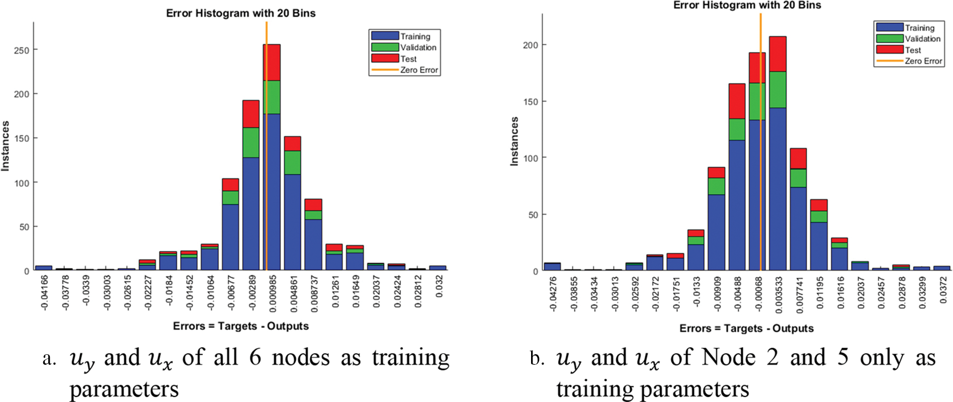
Figure 8: Error histogram of training using based on biaxial approach using Levenberg-Marquardt method with pure linear transfer function
The neural network model that is trained based on the hole in an infinite-width plate problem will be used to predict the maximum stresses on a hole in a finite-width plate problem. In the infinite-width model, the side wall is far from the hole such that there is no interaction between the stress concentration of the hole with the free edge on the side. However, with the finite-width geometry, the hole is closer to the free edge on the side. As a result of the interaction between the hole and the free edge, the stress concentration of the hole would increase. The analysis of the finite-width model is to evaluate if supervised learning can be used to support the finite element method to calculate stress accurately with an alternate geometry with coarse mesh size. Tests are conducted for a range of
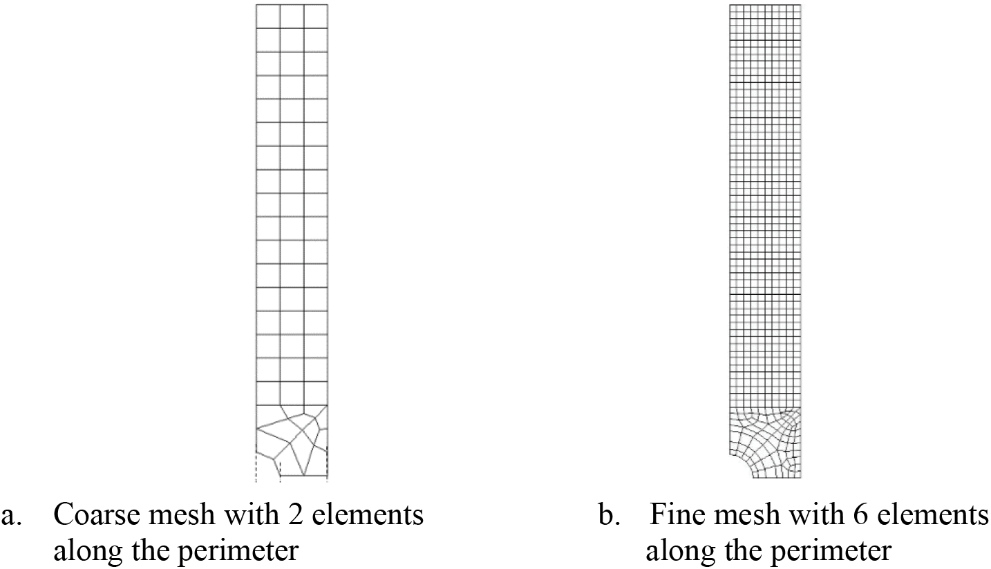
Figure 9: Coarse and fine mesh of a quarter-hole with finite-width of
The mesh is constructed by linear elements and only has 2 elements at the quarter-hole perimeter. The result is compared against the Roark’s solution [31] given as follows:
where
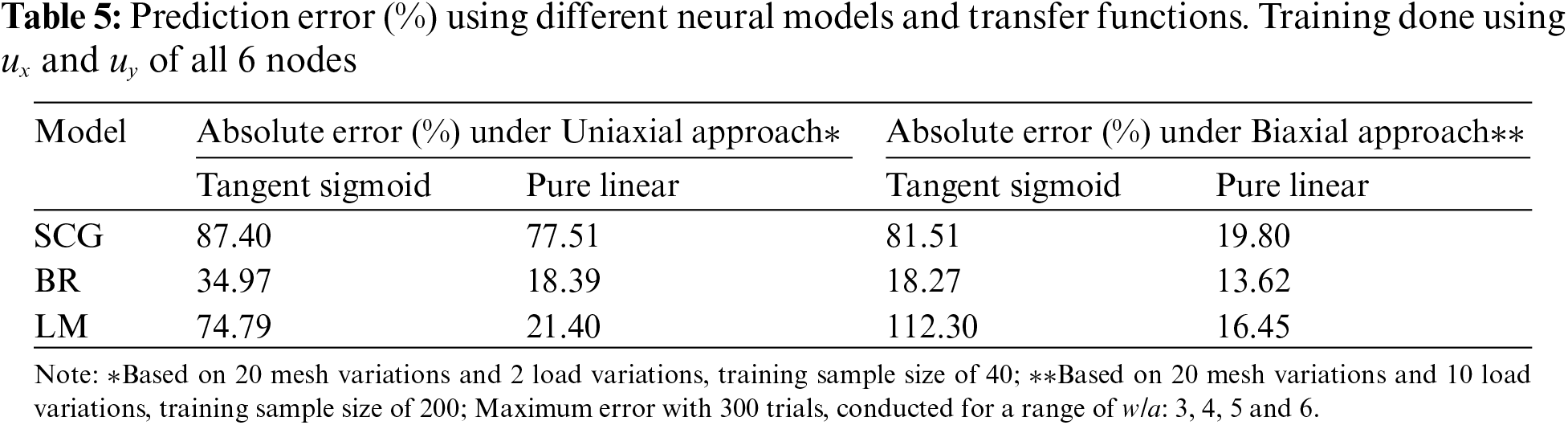
The result in Table 5 shows the prediction errors using the neural network model based on both
To evaluate if the trained model can be further improved by focusing the training on just the element with the highest stress, the training is based on
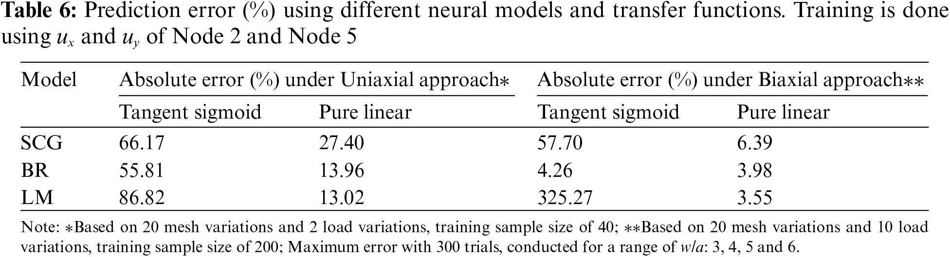
In Table 7, the stress concentration,
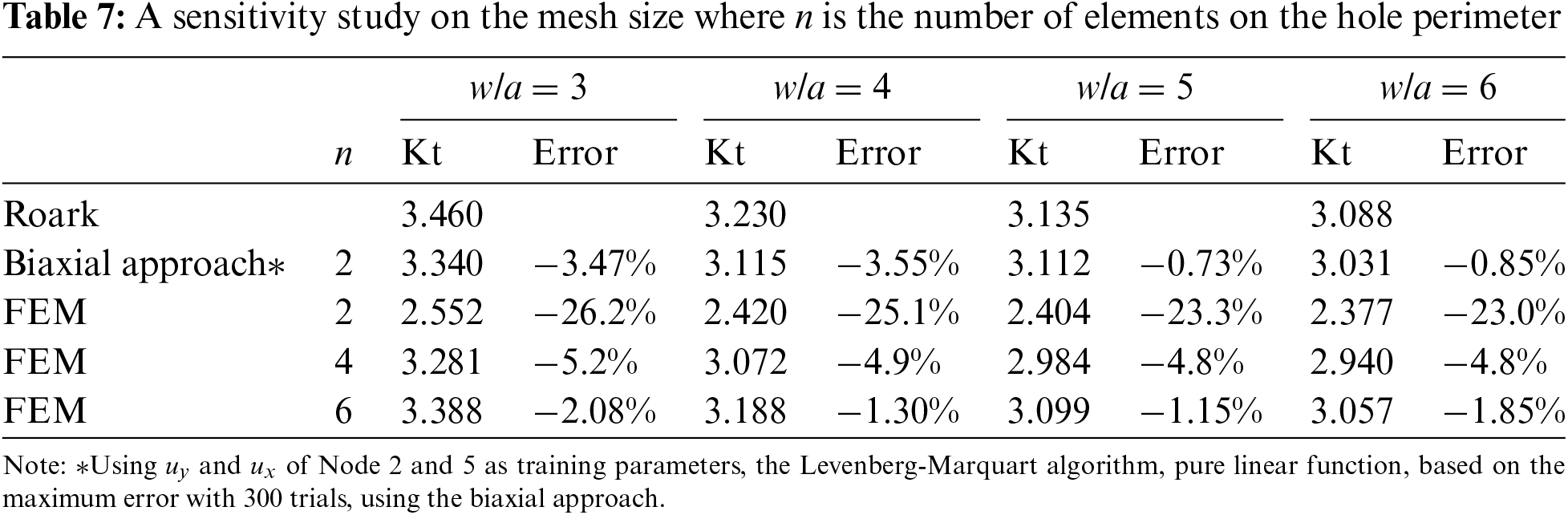
Both the LM and BR methods offer comparable results. Since the LM method has lower computational costs, the LM method would be the preferred method. The LM method will thus be applied on mesh with very different configurations such as multiple holes and staggered holes on finite-width plates for further tests. The biaxial approach will be used since it offers lower error than the uniaxial approach and has the advantage of being sensitive to biaxial loads.
4.3 Multiple Holes on Finite-Width Plate
The holes are separated by distance, d, from edge to edge of holes as shown in Fig. 10. To evaluate the accuracy of the prediction, the Kt values are obtained from the fine mesh using quadratic element Plane 183 as shown in Fig. 10b [9]. These Kt values are compared to the Kt values predicted by the neural network using displacements from coarse mesh shown in Fig. 10a. The variations in the mesh are shown in Table 8, with a fixed w/a = 5.
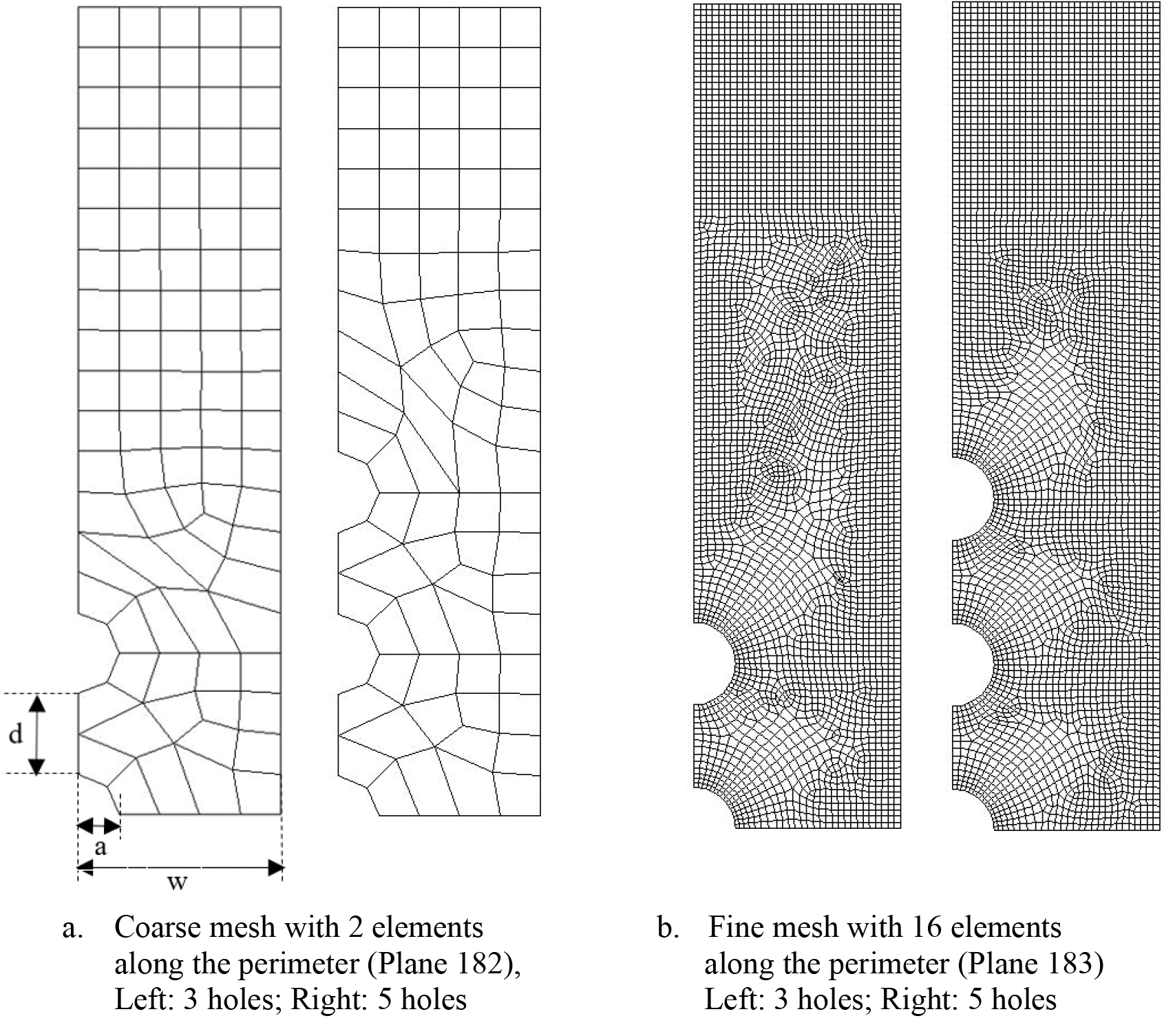
Figure 10: Coarse and fine mesh of multiple holes with finite-width of
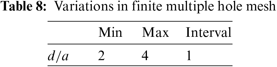
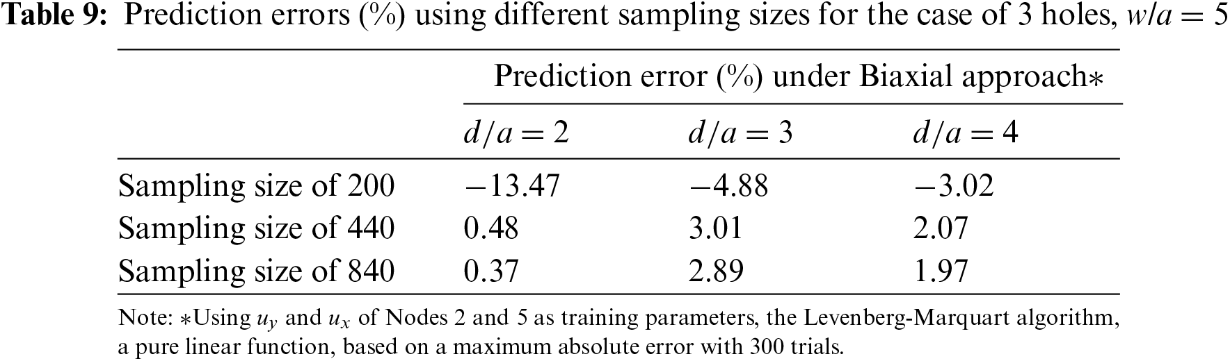
Table 9 investigates the minimum number of training sampling sizes needed to obtain good predictions for mesh with different configurations using biaxial-trained NN. To allow the NN to fit more loosely to the single hole in an infinite plate problem,
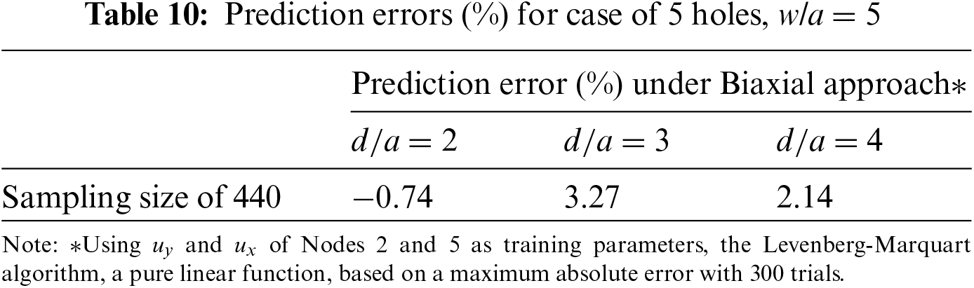
To ensure that the NN is also effective in predicting similar problems, the prediction error of a quarter finite plate with 3 holes as shown in Fig. 10 is studied. Table 10 shows that errors are generally higher than those in Table 9. However, the difference is not significant.
A sensitivity study will be conducted for the case of 5 holes since it has higher prediction errors. Table 11 shows that even for 5 holes, to achieve similar accuracy, a fine mesh with 6 elements along the perimeter as shown in Fig. 11 would be necessary. The prediction errors in Table 11 are low and comparable to that of the single hole in finite-width plate problem. This is because of the absence of any stagger of the holes which may introduce additional shear stresses. Therefore, the stress field is still similar to that of a single-hole problem. As a result, the trained NN model will still be able to make satisfactory predictions in this problem. Furthermore, a w/a of 5 is used in this problem. With higher w/a, the prediction error is expected to be low as it has higher similarity with the infinite-width problem that is used to train the NN.
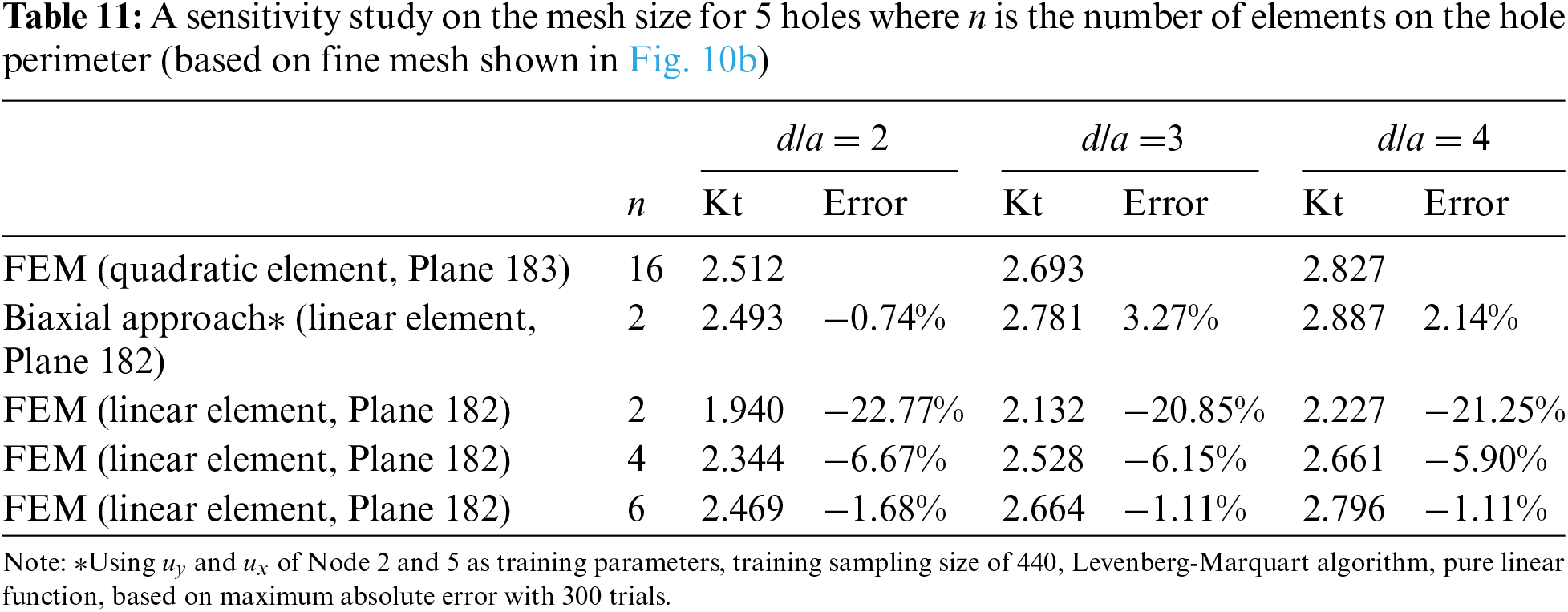
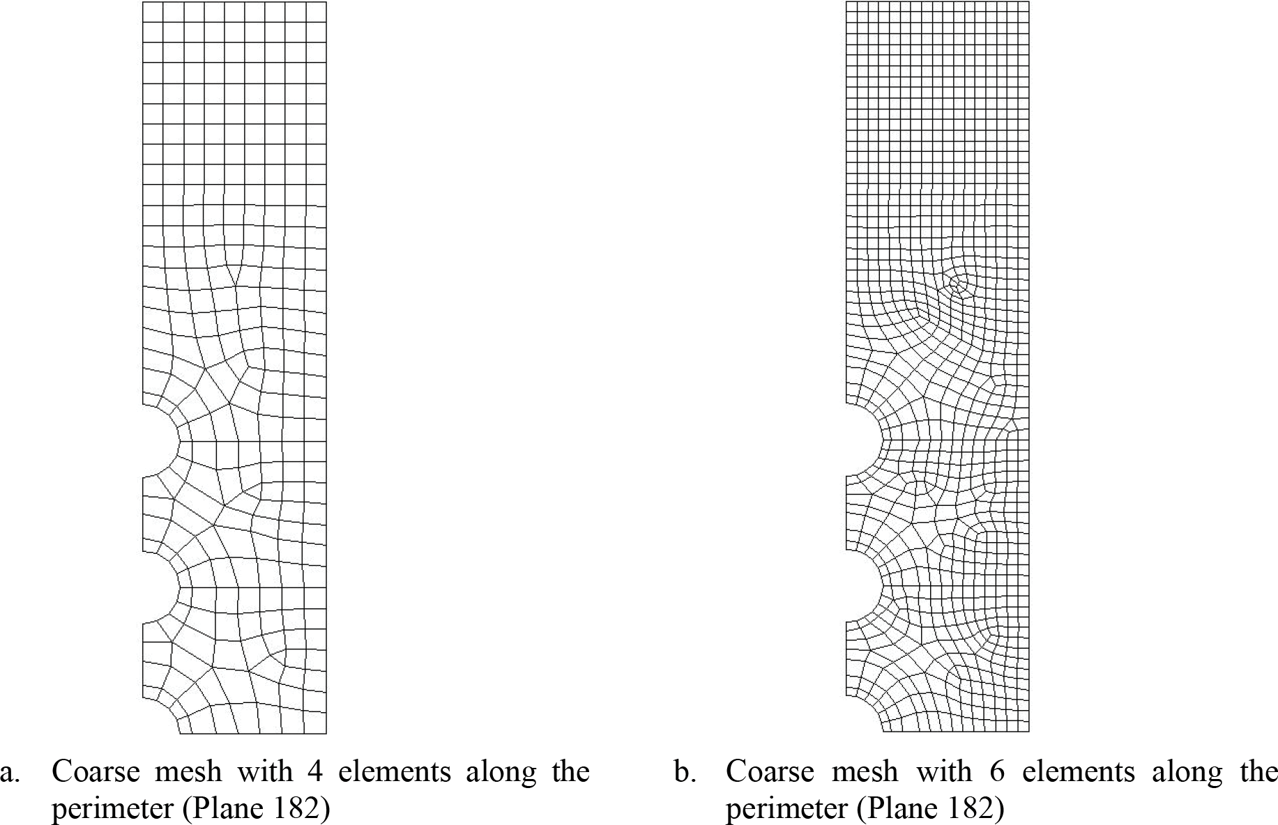
Figure 11: Various fine mesh of 5 holes
4.4 Staggered Holes on Finite-Width Plate
There is a stagger of s = 2 * radius of the hole. From Fig. 12a, only the elements adjacent to the quarter-hole are relevant. The mesh distortions away from the quarter-hole are inconsequential. Like the previous section, the Kt values of fine mesh shown in Fig. 12b are compared to the Kt values predicted by the neural network using displacements from coarse mesh. The variations of the mesh are shown in Table 12 with a fixed w/a = 5.
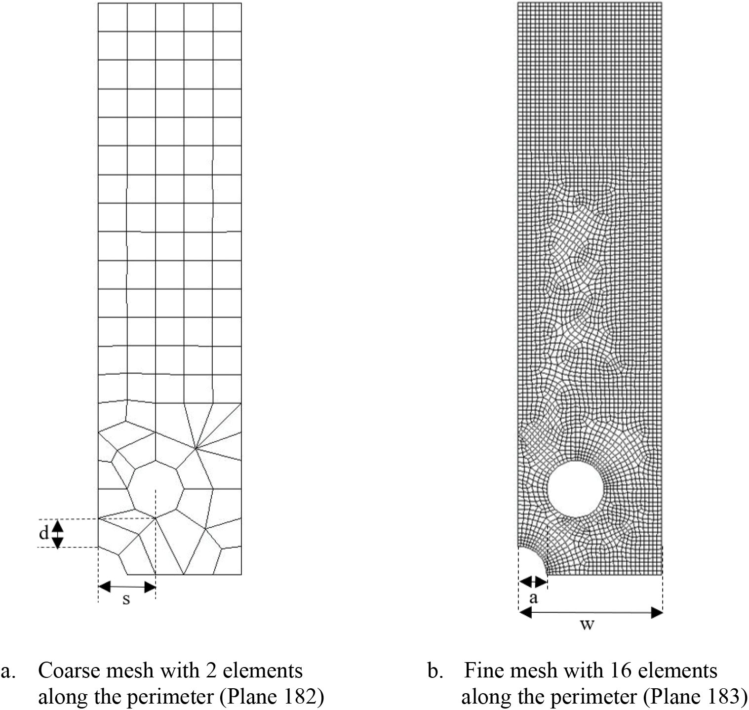
Figure 12: Coarse and fine mesh of staggered holes with finite-width of

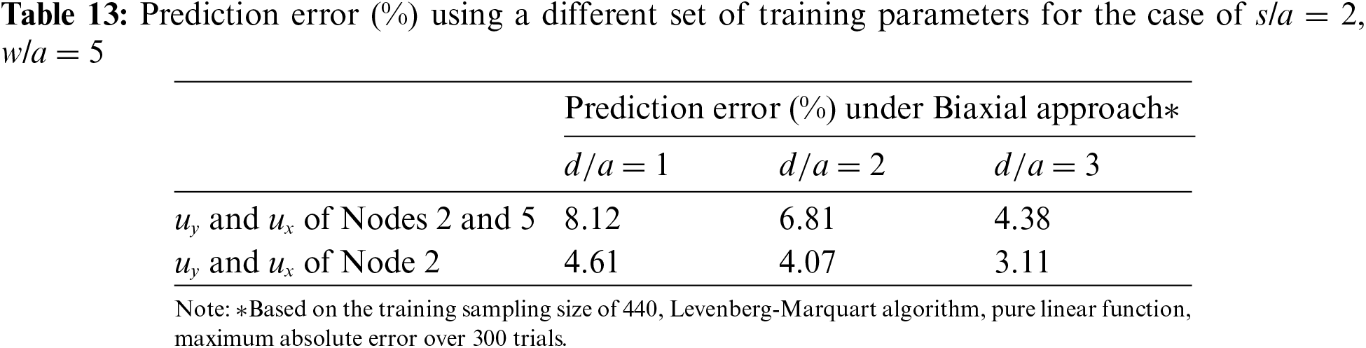
Since Node 5 is in the vicinity of the other hole, its stresses may be affected by the stress field of the other hole. This may increase discrepancies from that of a single hole. Table 13 evaluates if prediction error can be reduced by removing Node 5 from the training parameters. Indeed, prediction errors are lowered by using
Similar to Table 9 in Section 4.5, Table 14 shows that a sampling size of 440 lines offers a significant improvement over 200 lines while 840 lines offer little improvement.
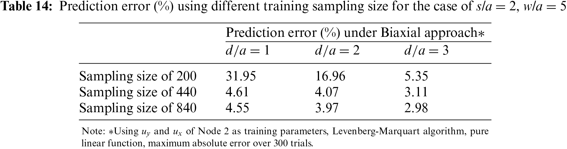
Table 15 shows that for s/a = 2, to achieve similar accuracy, a fine mesh with 6 elements along the perimeter shown in Fig. 13 would be necessary. The prediction errors are slightly higher than those for holes without stagger (Table 11) but are still satisfactory. This is due to the extra shear effect introduced by the staggered hole.
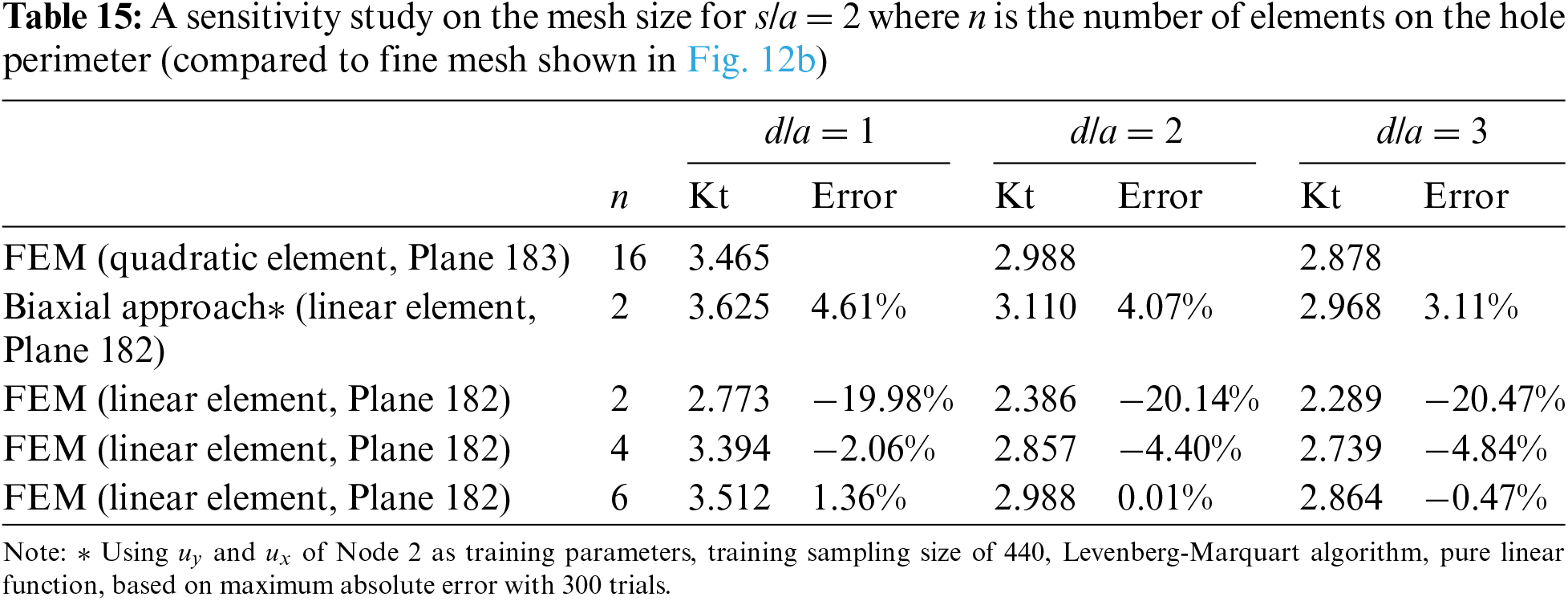
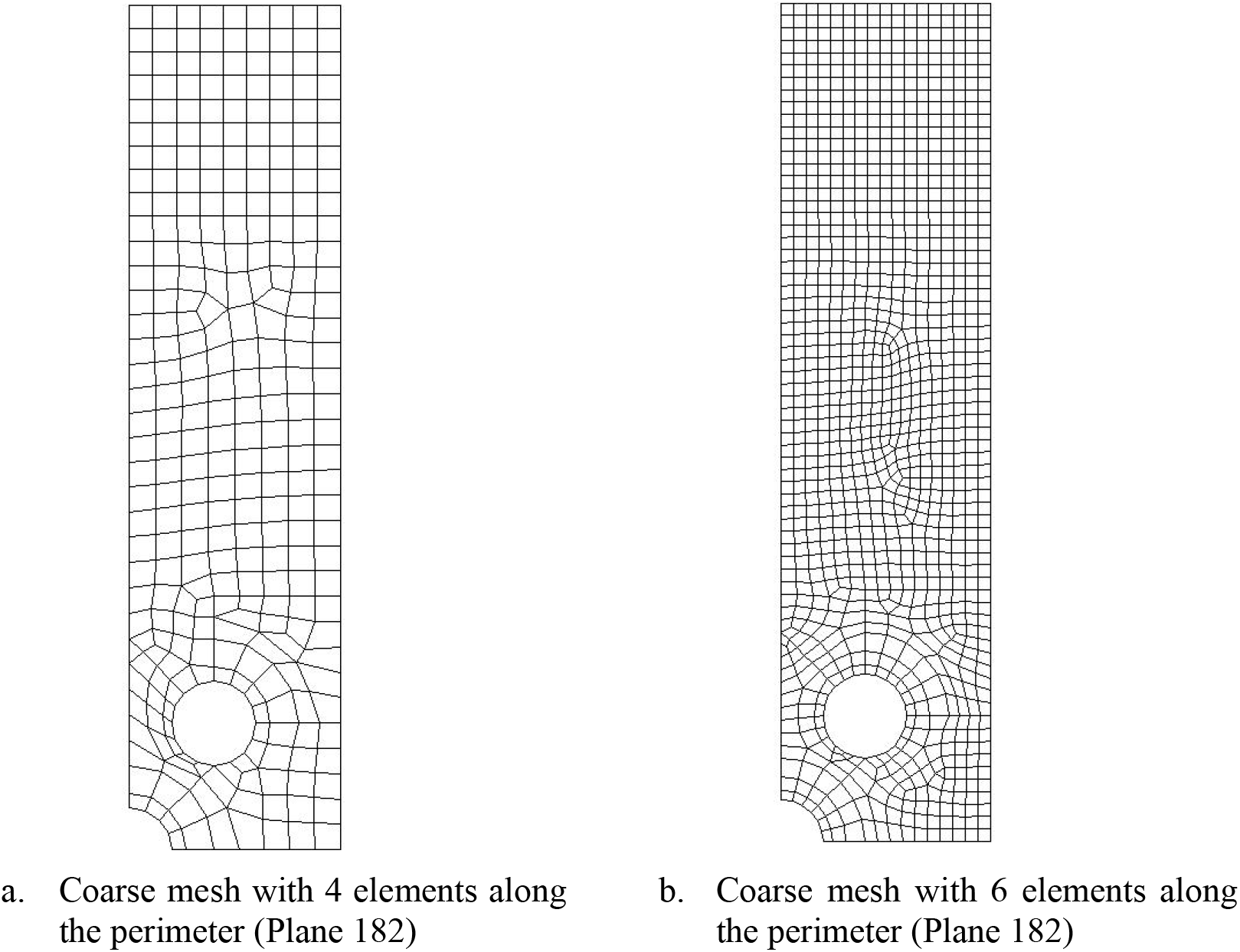
Figure 13: Various fine mesh of staggered holes with s/a = 2, w/a = 5
4.5 3D Single Hole in the Infinite Plate Using Biaxial Load Trained NN
The 3D mesh model is a quarter-hole in an infinite plate that is bisected in half along the z-axis. The coarse mesh is constructed with linear element Solid 185. Since this is the problem of predicting the stresses of a single hole in an infinite-width plate using a biaxial load trained NN like in Section 4.3,
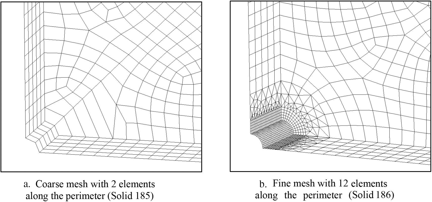
Figure 14: Coarse and fine mesh of 3D hole in infinite plate (w/a = 20) with thickness, t where t/a = 10
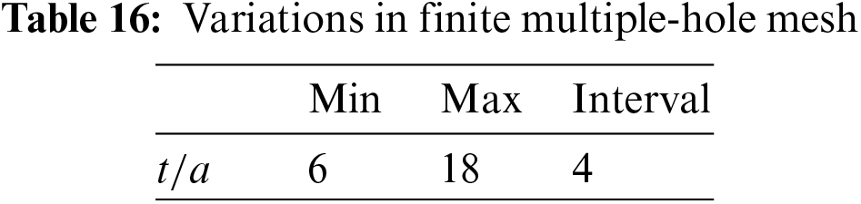
Table 17 shows that to achieve similar accuracy, a much finer mesh with 8 elements along the quarter-hole perimeter is required as shown in Fig. 15. Furthermore, the mesh must be constructed by quadratic element Solid 186.
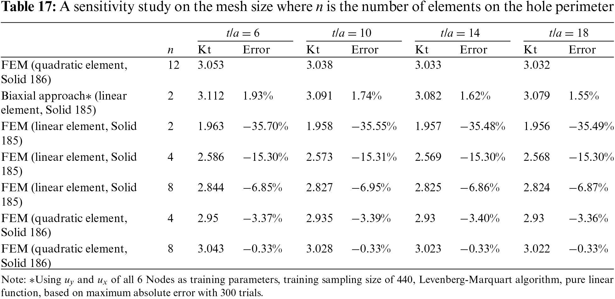
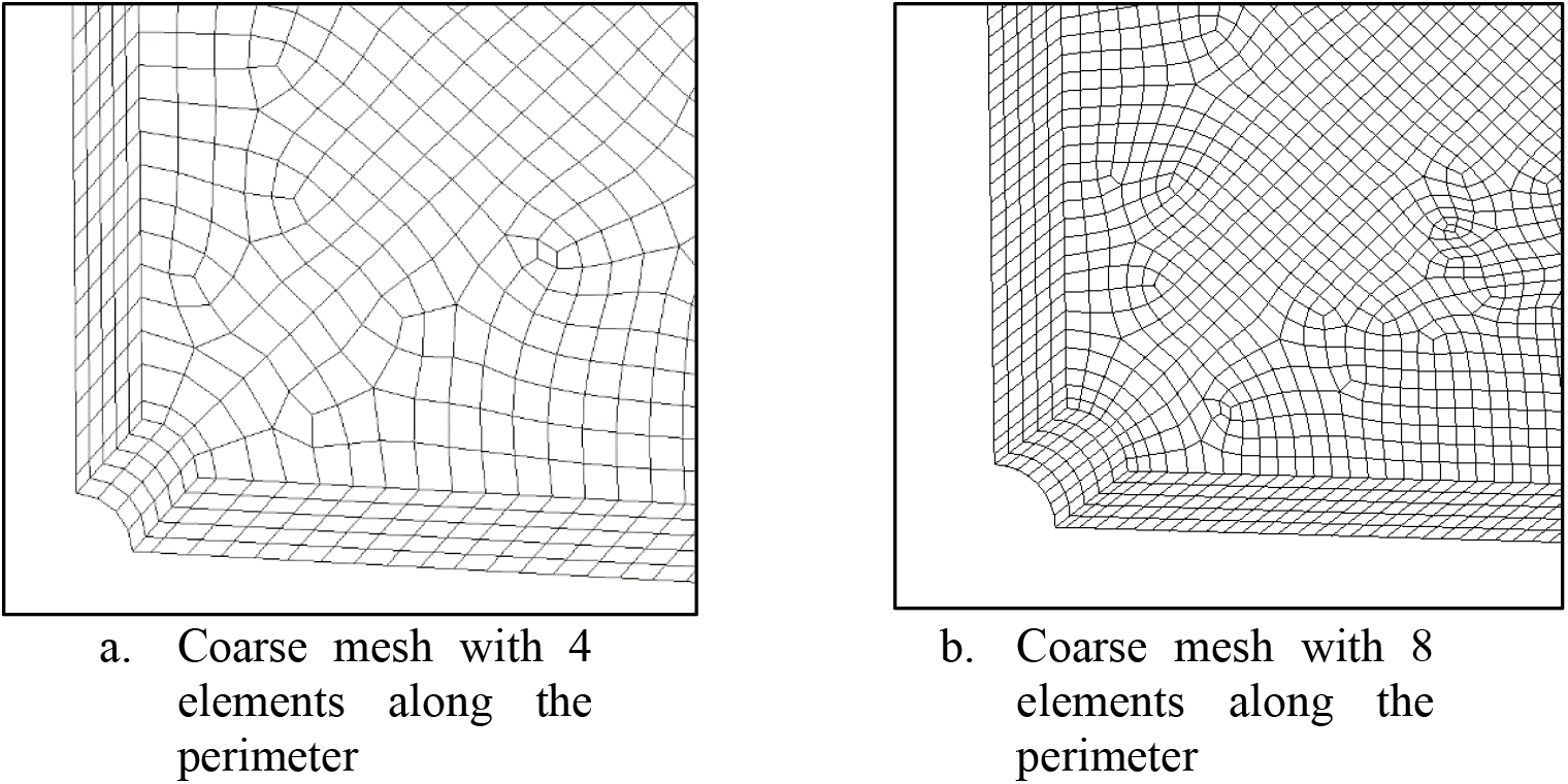
Figure 15: Various 3D fine mesh of single hole in infinite-width plate
The result shows that with the aid of supervised learning, an error of less than 5% can be obtained even for a coarse mesh with only 2 elements along the whole quarter perimeter. Training is done using the analytical solution for a coarse 2D mesh of a single hole in an infinite-width plate (2D). The prediction is successfully applied to different geometries such as holes in finite-width plates (2D), multiple holes without stagger (2D) and staggered holes (2D). A preliminary study done in this paper also demonstrates that the approach can be applied to 3D models with minor adjustments.
Levenberg-Marquardt method (LM) with pure linear transfer function and Bayesian Regularization (BR) with tangent sigmoid transfer function can achieve low prediction errors for the hole in infinite-width and finite-width problems. However, LM is faster and less calculational complex than BR. Thus, LM is extensively tested in this study. The result shows good prediction accuracy for the different problems.
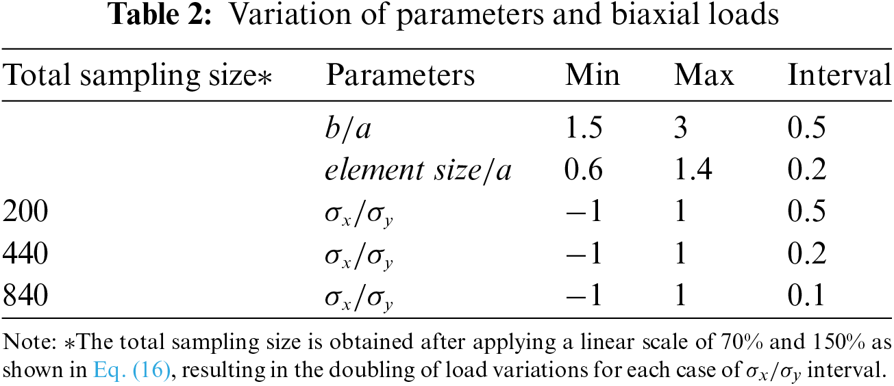
Nevertheless, various factors can affect the prediction results. Firstly, to train neural networks to be sufficiently sensitive to biaxial loading, the interval of
For staggered holes (2D), the prediction errors are higher due to the influence of shear stress which the neural network is not trained to model. In this case, the interaction of nearby holes may affect the prediction accuracy. Nodes chosen are encouraged to be further away from the other holes to reduce the influence of the stress field of the other adjacent holes. For example, for the staggered holes problem, removing the nodes that are in proximity of the adjacent hole from the training parameters drastically reduced the prediction errors to 4.61%. In contrast, conventional FEM with a coarse mesh of 2 elements at the quarter-hole perimeter has an error of 20.47%. To achieve similar accuracy by FEM without the aid of supervised learning, at least 6 elements at the quarter-hole perimeter would be necessary.
This paper has also demonstrated that the 3D problem consisting of a hole in an infinite-width 3D plate can be accurately predicted using supervised learning. The neural network training is performed using the 2D coarse mesh training set with generalized plane strain condition. When applied to the 3D plate that has a coarse mesh with just 2 elements at the quarter-hole perimeter, the maximum prediction error is 1.93%. In contrast, using the conventional FEM without any supervised training gives an error of 35.7%. To achieve similar accuracy by conventional FEM without supervised learning, more than 8 elements at the quarter-hole perimeter would be necessary.
Hence, it is demonstrated that supervised learning can be used effectively to aid finite element analysis such that even coarse mesh can offer satisfactory accuracy. As a result of using this approach, when performing complex 3-D design iterations with many holes, the need to perform many sub-modeling analyses (for greater accuracy) is significantly reduced.
Acknowledgement: The authors thank the guidance and encouragement from Prof S.N. Atluri over the years.
Funding Statement: The authors received no specific funding for this study.
Author Contributions: The authors confirm their contribution to the paper as follows: Study conception and design: W.T. Chow; analysis and interpretation of results: J.T. Lau, W.T. Chow; draft manuscript preparation: J.T. Lau. All authors reviewed the results and approved the final version of the manuscript.
Availability of Data and Materials: Data will be available upon request.
Conflicts of Interest: The authors declare that they have no conflicts of interest to report regarding the present study.
References
1. M. F. Moller, “A scaled conjugate gradient algorithm for fast supervised learning,” Neural Netw., vol. 6, no. 4, pp. 525–533, 1993. doi: 10.1016/S0893-6080(05)80056-5. [Google Scholar] [CrossRef]
2. H. P. Gavin, The Levenberg-Marquardt Algorithm for Nonlinear Least Squares Curve-Fitting Problems. Durham: Department of Civil and Environmental Engineering, Duke University, 2019. [Google Scholar]
3. M. G. Shirangi and A. A. Emerick, “An improved TSVD-based Levenberg-Marquardt algorithm for history matching and comparison with Gauss-Newton,” J. Petrol. Sci. Eng., vol. 143, no. 3, pp. 258–271, 2016. doi: 10.1016/j.petrol.2016.02.026. [Google Scholar] [CrossRef]
4. P. S. Prerana and P. Sehgal, “Comparative study of GD, LM and SCG method of neural network for thyroid disease diagnosis,” Int. J. Appl. Res., vol. 1, no. 10, pp. 34–39, 2015. [Google Scholar]
5. M. Kayri, “Predictive abilities of Bayesian regularization and Levenberg-Marquardt algorithms in artificial neural networks: A comparative empirical study on social data,” Math. Comp. App., vol. 21, no. 2, pp. 20, 2016. doi: 10.3390/mca21020020. [Google Scholar] [CrossRef]
6. N. P. Jouppi et al., “In-datacenter performance analysis of a tensor processing unit,” in Proc. of the 44th Int. Symp. on Computer Architecture (ISCA), Toronto, Canada, 2017, pp. 1–12. [Google Scholar]
7. Y. M. A. Hashash, S. Jung, and J. Ghaboussi, “Numerical implementation of a neural network based material model in finite element analysis,” Int. J. Numer. Meth. Eng., vol. 59, no. 7, pp. 989–1005, 2004. doi: 10.1002/nme.905. [Google Scholar] [CrossRef]
8. L. Manevitz, A. Bitar, and D. Givoli, “Neural network time series forecasting of finite-element mesh adaptation,” Neurocomputing, vol. 63, no. 6, pp. 447–463, 2005. doi: 10.1016/j.neucom.2004.06.009. [Google Scholar] [CrossRef]
9. W. T. Chow, “Supervised learning for finite element analysis of holes under tensile load,” in Int. Conf. on Comp. & Experimental Eng. and Sci., Switzerland, Springer International Publishing, 2019, pp. 1329–1339. [Google Scholar]
10. C. M. Bishop, Neural Networks for Pattern Recognition. UK: Oxford University Press, 1995. [Google Scholar]
11. S. Haykin, Neural Networks: A Comprehensive Foundation. USA: Prentice Hall PTR, 1998. [Google Scholar]
12. H. Almuallim and T. G. Dietterich, “Learning with many irrelevant features,” Artif. Intell., vol. 91, pp. 547–552, 1991. [Google Scholar]
13. D. F. Gordon and M. Desjardins, “Evaluation and selection of biases in machine learning,” Mach. Learn., vol. 20, no. 1–2, pp. 5–22, 1995. doi: 10.1007/BF00993472. [Google Scholar] [CrossRef]
14. H. H. Tan and K. H. Lim, “Vanishing gradient mitigation with deep learning neural network optimization,” in 2019 7th Int. Conf. on Smart Computing & Communications (ICSCC), Sarawak, Malaysia, 2019, pp. 1–4. [Google Scholar]
15. S. Hochreiter, “The vanishing gradient problem during learning recurrent neural nets and problem solutions,” Int. J. Uncertain., Fuzzi. Knowled.-Based Sys., vol. 6, no. 2, pp. 107–116, 1998. doi: 10.1142/S0218488598000094. [Google Scholar] [CrossRef]
16. D. Nguyen and B. Widrow, “Improving the learning speed of 2-layer neural networks by choosing initial values of the adaptive weights,” in 1990 IJCNN Int. Joint Conf. on Neural Networks, San Diego, USA, 1990, pp. 21–26. [Google Scholar]
17. Matlab, Nguyen-Widrow Layer Intialization Function. USA: MathWorks, 2018. [Google Scholar]
18. A. Pavelka and A. Procházka, “Algorithms for initialization of neural network weights,” in Proc. of the 12th Annual Conf., MATLAB, 2004, pp. 453–459. [Google Scholar]
19. M. R. Wayahdi, M. Zarlis, and P. H. Putra, “Initialization of the Nguyen-widrow and Kohonen algorithm on the backpropagation method in the classifying process of temperature data in Medan,” J. Phy.: Conf. Series, vol. 1235, no. 1, pp. 012031, 2019. doi: 10.1088/1742-6596/1235/1/012031. [Google Scholar] [CrossRef]
20. J. Lundén and V. Koivunen, “Scaled conjugate gradient method for radar pulse modulation estimation,” in 2007 IEEE Int. Conf. on Acoustics, Speech and Signal Processing-ICASSP’07, Honolulu, USA, 2007, pp. II-297. [Google Scholar]
21. M. I. Lourakis, “A brief description of the Levenberg-Marquardt algorithm implemented by levmar,” Found. Res. Technol., vol. 4, no. 1, pp. 1–6, 2005. [Google Scholar]
22. K. Madsen, H. B. Nielsen, and O. Tingleff, Methods for Non-Linear Least Squares Problems. Denmark: Technical University of Denmark, 2004. [Google Scholar]
23. H. B. Nielsen, Damping Parameter in Marquardt’s Method. Denmark: Technical University of Denmark, 1999. [Google Scholar]
24. K. Levenberg, “Method for the solution of certain problems in least squares siam,” Q. Appl. Math., vol. 2, no. 2, pp. 164–168, 1944. doi: 10.1090/qam/10666. [Google Scholar] [CrossRef]
25. D. W. Marquardt, “An algorithm for least-squares estimation of nonlinear parameters,” J. Soc. Ind. Appl. Math., vol. 11, no. 2, pp. 431–441, 1963. doi: 10.1137/0111030. [Google Scholar] [CrossRef]
26. D. J. MacKay, “Bayesian interpolation,” Neural Comput., vol. 4, no. 3, pp. 415–447, 1992. doi: 10.1162/neco.1992.4.3.415. [Google Scholar] [CrossRef]
27. F. D. Foresee and M. T. Hagan, “Gauss-Newton approximation to Bayesian learning,” in Proc. of Int. Conf. on Neural Networks (ICNN’97), Houston, USA, 1997, pp. 1930–1935. [Google Scholar]
28. W. D. Pilkey, D. F. Pilkey, and Z. Bi, Peterson’s Stress Concentration Factors. USA: John Wiley & Sons, 2020. [Google Scholar]
29. ANSYS, Inc. Mechanical APDL Theory Reference. USA: ANSYS, Inc., 2018. [Google Scholar]
30. Matlab, Statistics and Machine Learning Toolbox: User’s Guide. USA: MathWorks, 2018. [Google Scholar]
31. W. C. Young, R. G. Budynas, and A. M. Sadegh, Roark’s Formulas for Stress and Strain. USA: McGraw-Hill Education, 2012. [Google Scholar]
Cite This Article
 Copyright © 2024 The Author(s). Published by Tech Science Press.
This work is licensed under a Creative Commons Attribution 4.0 International License , which permits unrestricted use, distribution, and reproduction in any medium, provided the original work is properly cited.
 Downloads
 Citation Tools