1 Introduction
Nonlocal models based on long-range interactions have broad applications in various research fields [1–5]. Differing from the classical modeling method for PDEs, nonlocal models employ integral-type operators instead of differential operators in space to establish more generalized integro-differential equations, which rely on the interaction between points within a finite distance. Due to their characteristics, nonlocal models can provide a more precise description in the presence of anomalous behaviors, discontinuities, and singularities, which are challenging for partial differential equation models. In particular, the peridynamic (PD) model proposed by Silling [1] allows for discontinuities in the displacement field and has been successfully applied to fracture and damage for diverse materials and structures [4,6,7]. Moreover, nonlocal diffusion models can depict much more general stochastic jump processes relative to Brownian motion corresponding to normal diffusion [8,9], which allows for discontinuities and jump behaviors. Nonlocal diffusion models can also describe widespread analogous diffusion by selecting some special nonlocal operators, such as fractional derivative operators [10].
Although nonlocal models exhibit a better modeling capability for complex physical phenomena than classical local models, they need to deal with an additional layer of integration, which results in algebraic systems having higher computational and assembly costs. Besides, one has to face higher solving costs of discrete systems due to much lower sparsity than that for PDEs. Thus, it is urgent to develop efficient numerical methods for solving nonlocal problems. There have been great efforts on fast algorithms for solving various high-dimensional systems, and one of the most widely used methods is model reduction based on proper orthogonal decomposition (POD) and Galerkin projection [11,12]. The POD technique [13] can significantly decrease the degrees of freedom of classical numerical methods, and has been applied to various fields of PDE problems, such as computational fluid dynamics (CFD) [12,14], compressible fluid flow as well as incompressible fluid flow [15,16], phase field [17], miscible displacement [18], supersonic flow [19], hydraulic fracturing [20,21] and so on.
In recent years, there also have been some efforts to develop reduced-order methods for nonlocal models. Gunzburger et al. [22] applied the POD method to the parametrized time-dependent nonlocal diffusion problem in the 1D case and trained a system with only a few degrees of freedom using parameterized equations, achieving almost the same accuracy as finite element discrete models. A POD-based fast algorithm was developed for one-dimensional nonlocal parabolic equations and nonlocal wave equations, which vastly speeds up the process of solving algebraic systems while maintaining high accuracy [23]. Considering that Galerkin methods need to compute multiple integrals, a reduced-order fast reproducing kernel collocation method is proposed to solve 2D nonlocal diffusion equations and peridynamic equations [24]. In this method, to get rid of the high computational complexity in the projection of inhomogeneous volume constraints, a mixed reproducing kernel approximation with nodal interpolation property is introduced to make the projection explicit, thereby truly improving computational efficiency without compromising accuracy.
Nevertheless, to our knowledge, there are very few works on the relevant theoretical analysis of POD reduced-order algorithms for nonlocal problems with finite element methods or meshfree methods. Thus, by drawing inspiration from ideas similar to those used in classical numerical analysis methods and leveraging existing techniques on analysis of POD-based reduced-order methods for PDEs, we demonstrate the existence, stability, and convergence of the POD reduced-order solutions for nonlocal models through different methodologies, and supply several numerical experiments to validate the theoretical results.
The rest of the paper is organized as follows. In Section 2, we introduce the nonlocal diffusion model with Dirichlet volume constraints and a finite scope of nonlocal interactions. In Section 3, we briefly derive the weak form for the nonlocal diffusion equation, and then give its finite element discretization, including the handling of mesh partitioning for nonlocal domains as well as the quadrature on an Euclidean ball, and provide some significant theoretical conclusions. The reduced-order model constructed by POD for nonlocal diffusion equations is given in Section 4, and we present the existence and stability analysis as well as the error estimates for the reduced-order solutions. In Section 5, we provide several numerical tests to verify the accuracy and efficiency of the reduced-order method and explore the effect of various parameters on the performance of the algorithm. Conclusions and summaries are given in Section 6.
2 Nonlocal Diffusion Model
The mathematical definitions and corresponding notations that are used throughout the article will be first introduced. Let Ω⊂Rd denote a bounded open domain, and we define its corresponding interaction domain
Ωℐ={y∈Rd∖Ω:∃x∈Ω s.t.‖x−y‖≤δ},(1)
where δ>0 describes the scope of nonlocal interaction, which is often referred to as the horizon or interaction radius. In geometric terms, Ωℐ is generally a strip-shaped region with thickness δ surroundin Ω, and Fig. 1 shows an example of the interaction domain in a 2D case.

Figure 1: The nonlocal interaction domain
We consider the following unsteady nonlocal diffusion problem with Dirichlet volume constraints:
{∂u∂t−ℒΔu(x,t)=f(x,t),on Ω×(0,T],u(x,t)=g(x,t),on Ωℐ×(0,T],u(x,0)=u0(t),on Ω∪Ωℐ,(2)
where f, g, u0 are given functions, ℒδ represents a nonlocal diffusion operator with finite range of interaction defined as
ℒδu(x,t)=2∫Bδ(x)(u(y,t)−u(x,t))γδ(x,y)dy,∀x∈Ω,t≥0,(3)
and γδ(x,y):Rd×Rd→R is called the kernel function, which is generally a nonnegative and symmetric function. Driven by the reality, the support of the kernel is usually limited to be over a bounded region Bδ(x), which contains the points in Ω∪Ωℐ interacting with x∈Ω, i.e., only if y∈Bδ(x). For the interaction region Bδ(x), we focus on the specific choice of Euclidean balls centered at x with radius δ, as used in [25].
Without loss of generality, we also assume in this paper that the kernel γδ(⋅,⋅) is square-integrable and translation invariant, i.e., γδ(x,y)=γδ(x−y).
3 Finite Element Method for Nonlocal Diffusion Problems
3.1 Weak Formulation
The weak formulation of the nonlocal problem (2) can be derived by the same procedure as the classical PDE setting. Applying Green’s first identity of the nonlocal vector calculus [26] with a test function v(x) vanishing on Ωℐ yields
∫Ω∂u∂tv(x)dx+∫Ω′∫Ω′(u(y,t)−u(x,t))(v(y)−v(x))γδ(x,y)dydx=∫Ωf(x,t)v(x)dx,(4)
where Ω′=Ω∪Ωℐ, then it can be simplified as
(ut,v)+A(u,v)=F(v),(5)
where A(u,v) is the symmetric nonlocal bilinear form as follows:
A(u,v):=∫Ω∪Ωℐ∫Ω∪Ωℐ(u(y,t)−u(x,t))(v(y)−v(x))γδ(x,y)dydx,(6)
and F(v) denotes the linear functional
F(v):=∫Ωf(x,t)v(x)dx.(7)
Based on Eq. (6), we can define the energy norm |||v||||:=A(v,v), and introduce the following nonlocal energy spaces:
{V(Ω∪Ωℐ)={v∈L2(Ω∪Ωℐ):|||v||||<∞},Vc(Ω∪Ωℐ)={v∈V(Ω∪Ωℐ):v=0 on Ωℐ}.(8)
Therefore, the weak formulation of the nonlocal problem (2) can be defined as follows:
Given f(⋅,t)∈L2(Ω), g(⋅,t)∈L2(Ωℐ) and u0∈L2(Ω∪Ωℐ), find u(⋅,t)∈V(Ω∪Ωℐ), for any t∈(0,T], such that u(⋅,t)=g(⋅,t) for x∈Ωℐ and
{(ut,v)+A(u,v)=F(v),∀v∈Vc(Ω∪Ωℐ),u(x,0)=u0(x),x∈Ω∪Ωℐ.(9)
The well-posedness results for the problem (9) have been supplied in previous references [9,10,25,27].
3.2 Finite Element Grid for Nonlocal Domain
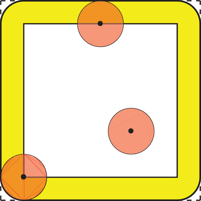
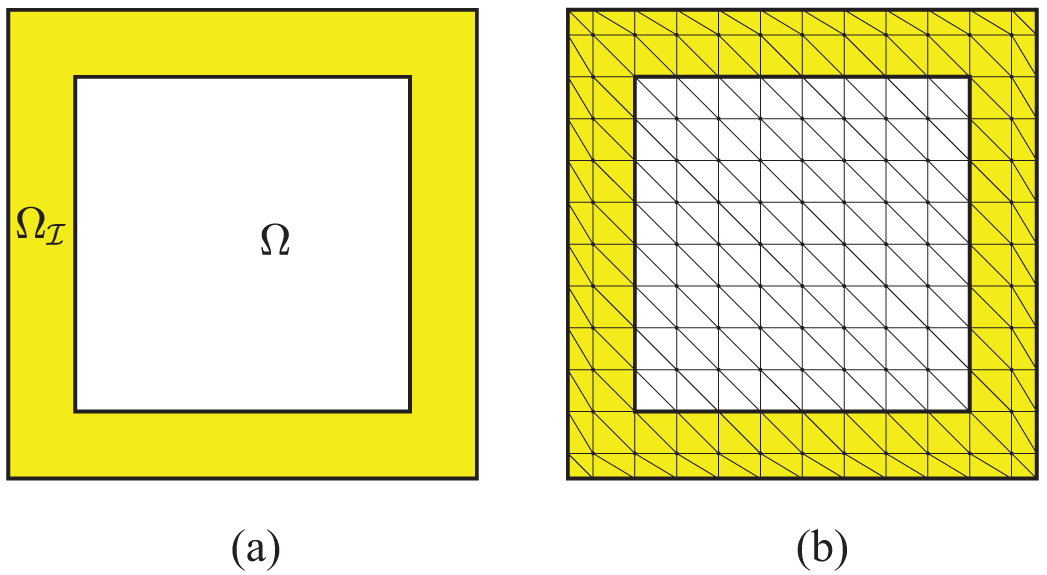
We assume that Ω is a polygonal domain. Let 𝒯h,Ω denote a regular triangulation of Ω with KΩ elements {ℰk}k=1KΩ, referred to as simplices, and 𝒯h,Ω is an exact triangulation due to Ω. In contrast to the scenario of local PDEs, there exists a boundary domain Ωℐ with non-zero volume in the nonlocal setting, which also requires subdivision. However, the Euclidean ball will cause rounded corners to Ωℐ, so the corresponding interaction domain is generally not polyhedral, which may lead to inexact triangulation for Ωℐ. Fig. 2 takes a rectangular domain for example. One way introduced in references [28,29] to solve this problem is to approximate Ωℐ using a polyhedral domain by replacing rounded corners with right angles (see the dashed line in Fig. 2), and we will regard this approximate domain as Ωℐ in the remainder of this paper.

Figure 2: A rectangular domain Ω and the corresponding interaction domain Ωℐ with rounded corners in solid lines and right angle in dotted lines
Then we denote 𝒯h,Ωℐ as an exact regular triangulation of Ωℐ with KΩℐ elements {ℰk}k=KΩ+1KΩ+KΩℐ. It should be noted that, for nonlocal case, the triangulation of Ω and Ωℐ need to satisfy several conditions as follows [29]:
• every vertex of Ω and Ωℐ should be a vertex of 𝒯h,Ω or 𝒯h,Ωℐ;
• all elements {ℰk}k=1KΩ+KΩℐ cannot stretch across the common boundary of Ω and Ωℐ;
• the vertices of the triangulations of 𝒯h,Ω and 𝒯h,Ωℐ must coincide along the boundary ∂Ω.
As a result, the triangulation of the entire domain Ω∪Ωℐ can be represented as 𝒯h=𝒯h,Ω∪𝒯h,Ωℐ with elements {ℰk}k=1KΩ+KΩℐ.
3.3 Finite Element Discretization
In this subsection, we consider the finite element discretization of the weak Eq. (9) using continuous piecewise-polynomial spaces, and restrict ourselves to Lagrange-type basis functions defined on a set of nodes. Let {xj}j=1J denote the nodes associated with the above triangulation 𝒯h. More specifically, the nodes {xj}j=1JΩ are located in Ω, {xj}j=JΩ+1J are located in Ωℐ, and contain the nodes on ∂Ω as well. Let ϕj(x)(j=1,2,…,J) denote the piecewise polynomial functions satisfying ϕj(xi)=δij. Then we define finite element subspaces Vh(Ω∪Ωℐ)⊂V(Ω∪Ωℐ) and Vch(Ω∪Ωℐ)⊂Vc(Ω∪Ωℐ), which are spanned by bases {ϕj(x)}j=1J and {ϕj(x)}j=1JΩ, respectively.
Let uh(x,t)∈Vh denote the finite element approximation of the solution u(x,t) of the problem (2), gh(x,t) be the interpolation of g(x,t) in the space Vh∖Vch and u0h(x)∈Vh be the interpolation approximation to u0(x). Then, the finite element discretization of the weak formulation can be defined as follows: for any t∈(0,T], seek uh(t)∈Vh(Ω∪Ωℐ) such that uh=gh for x∈Ωℐ and
{(uth,vh)+A(uh,vh)=F(vh),∀vh∈Vch(Ω∪Ωℐ),uh(x,0)=u0h(x),x∈Ω∪Ωℐ.(10)
The finite element approximation uh∈Vh can be expressed as
uh(x,t)=∑j=1Juj(t)ϕj(x),(11)
and from the properties of basis functions, we have uh(xj,t)=uj(t).
We substitute Eq. (11) to Eq. (10) and let vh go through the test function space Vh, obtaining a system of linear equations as follows:
∑j=1J(ϕj(x),ϕi(x))∂uj∂t+∑j=1‘JA(ϕj(x),ϕi(x))uj(t)=F(ϕi(x),t),i=1,2,⋯,J,(12)
where uj(t),j=1,2,⋯,J are the unknown coefficients of finite element solutions, which are time-dependent with 0<t≤T. Let X(t)=[uj(t)]j=1J denote the coefficient vectors, and then the system (12) can be written as the following equivalent matrix form:
{MX′(t)+AX(t)=b(t),X(0)=[u0(x1),u0(x2),⋯,u0(xJ)]T.(13)
where the mass matrix is M=[ϕj(x),ϕi(x)]i,j=1J, the stiffness matrix is A=[A(ϕj(x),ϕi(x))]i,j=1J and the load vector is b(t)=[F(ϕi(x),t)]i=1J. The system (13) can be regarded as a system of ordinary differential equations (ODEs) about time t and is also called the semi-discretization scheme in spatial direction.
3.4 Balls Approximation for Stiffness Matrix Computing
Differing from the local PDEs whose stiffness matrices only involve a single integral, the stiffness matrices of nonlocal equations contain double integrals as follows:
A(ϕj,ϕi)=∫Ω∪Ωℐ∫Ω∪Ωℐ(ϕj(y)−ϕj(x))(ϕi(y)−ϕi(x))γδ(x,y)dydx=∑k=1K∫ℰk∫Bδ(x)(ϕj(y)−ϕj(x))(ϕi(y)−ϕi(x))γδ(x,y)dydx.(14)
In Eq. (14), the inner integral is defined on Euclidean balls, which may cause much more difficulties for the computation and assembly process and may result in a loss of the convergence order, since classical quadrature rules, such as Gauss quadrature, cannot be performed well on that curved domain.
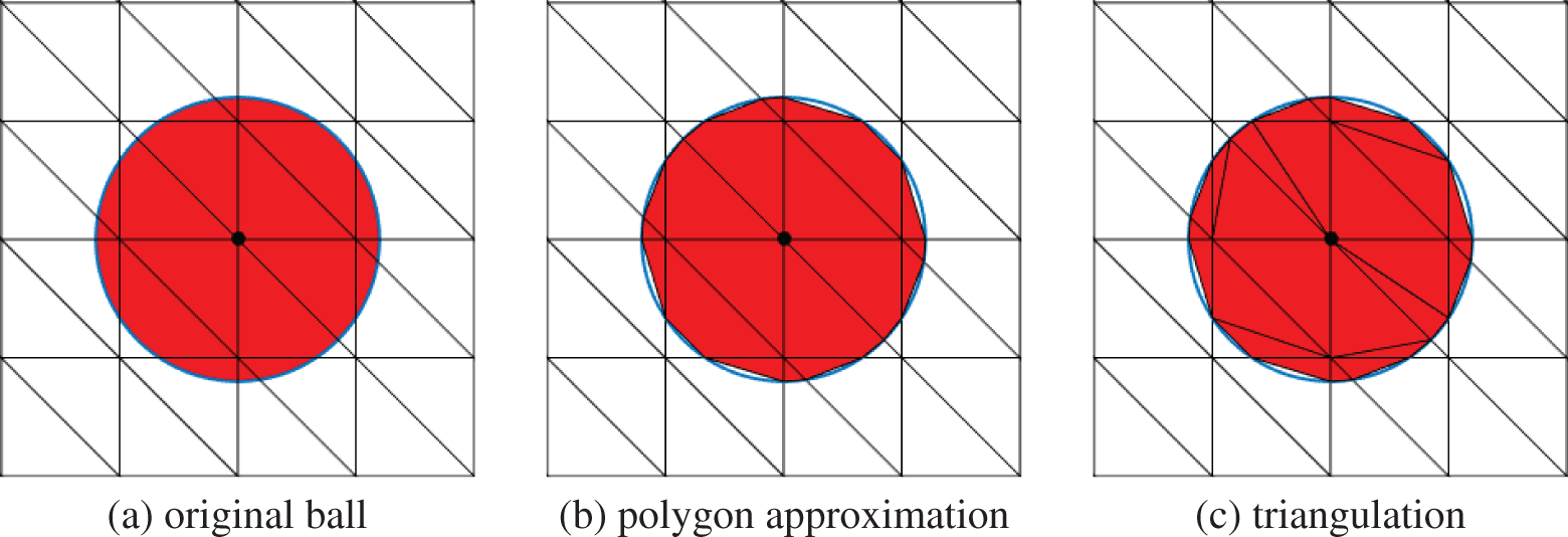
To overcome these difficulties, D’Elia et al. [29] used polyhedral approximate balls denoted by Bδ,h(x) to replace the original Euclidean ball Bδ(x), and the construction of the approximate balls is based on the geometric relationship between the finite element grid 𝒯h and the Euclidean ball Bδ(x). Besides, Lu et al. [30] exploited polar coordinate transformation to translate the spherical neighborhood Bδ(x) in cartesian coordinates to a rectangular region in polar coordinates based on a localized collocation method. In reference [29], the authors proposed several different ball approximation strategies, from which we select the nocaps strategy in this paper. Besides, this strategy has been proven to have a geometric error of 𝒪(h2), thus, it does not impact the convergence order when using piecewise linear elements.
The nocaps strategy is briefly outlined here. To begin with, we seek the simplices ℰk that are wholly or partially contained within the ball, and calculate the intersection points of the boundary of the ball and the sides of the above simplices. We then construct a polyhedral region using these points as vertices. Finally, the polyhedral domain is subdivided into several simplices exactly. Fig. 3 illustrates the sketch of the nocaps approximate strategy in 2D.

Figure 3: Sketch of construction of nocaps polyhedral approximate ball
Consequently, substituting Bδ,h(x) for Bδ(x) in (14), we have
A(ϕj,ϕi)= ∑k=1K∑k′=1K′∫ℰk∫ℰ′k′ (ϕj(y)−ϕj(x))(ϕi(y)−ϕi(x))γδ(x,y)dydx,(15)
where ℰk′′⊂ℰk∩Bδ,h(x)⊂ℰk∩Bδ(x). As seen in Eq. (15), the inner integral can be written as the sum of integrations over the above simplices, which can be computed by utilizing classical Gaussian quadrature rules without loss of accuracy.
3.5 Full-Discrete Schemes
We define a uniform partition for the time interval [0,T] with a step size Δt. Discreting the ODEs in Eq. (13) by θ−scheme yields
MXn+1−XnΔt+θAXn+1+(1−θ)AXn=θbn+1+(1−θ)bn,(16)
where Xn denotes the solution vectors at the time instant t=nΔt. Let N=T/Δt denote the number of time steps, then Eq. (16) can be simplified as
A∼Xn+1=b∼n+1,n=0,1,⋯,N−1,(17)
where
A∼=MΔt+θA,(18a)
b∼n+1=θbn+1+(1−θ)bn+MΔtXn−(1−θ)AXn.(18b)
One can observe that, for the system (17), different values of θ lead to different schemes. To be specific, taking θ=1 can get the implicit back-Euler scheme, and taking θ=0 can get the explicit forward-Euler scheme. It has been proven that both two schemes have the first-order accuracy. In this paper, we choose θ=0.5 corresponding to the well-known Crank-Nicolson scheme for the linear system (17). To mitigate the impact of geometric errors on convergence, in the following discussion, we exclusively employ piecewise linear elements to solve nonlocal equations. We next give some theoretical results for the full-discrete schemes.
Lemma 3.1. [31] If the solution u of the problem (2) is sufficiently smooth, then the Crank-Nicolson scheme of the system (17) for the nonlocal diffusion equation in Eq. (2) is unconditionally stable and satisfies the following error estimate:
‖u(x,tn)−uhn(x)‖L2(Ω∪Ωℐ)≤C(h2+Δt2),(19)
where C is a positive constant independent of the mesh size h and the time step Δt, and uhn(x) denote the finite element approximations of the true solution u at tn=nΔt, i.e., uhn(x)=uh(x,tn)=∑j=1Juj(tn)ϕj(x),n=0,1,⋯,N.
4 Reduced-Order Model Based on POD for Nonlocal Diffusion Problems
In this section, we first present the procedure of model reduction for nonlocal diffusion problems using the POD method and Galerkin projection. Then, the existence, stability, and convergence of the reduced-order solutions will be deduced.
4.1 Establishment of the Reduced-Order Model
We first select the initial k solution vectors X1,X2,⋯,Xk(k≪N) as snapshots by solving the finite element system (17) in a small interval [0,tk]. One significant issue in using POD methods for the nonlocal problem is to handle inhomogeneous volume constraints, and the approaches to treating time-dependent inhomogeneous Dirichlet boundary conditions for PDEs when using POD methods have been proposed in reference [32], which can also be applied to inhomogeneous volume constraints for the nonlocal setting.
After getting the set of snapshots {Xn}n=1k, each of them satisfies the volume constraints in Ωℐ at a certain moment. To guarantee that the reduced-order solutions can be expressed as a linear combination of POD bases and meet the inhomogeneous volume constraints in the meanwhile, one should correct original snapshots to obtain a set of modified snapshots {un}n=1k that satisfy homogeneous volume constraints. The modified snapshots can be simply obtained by un=Xn−unps, where unps denote vectors whose components are the function values of particular solutions ups(x,t) on finite element nodes at the time instant tn. The particular solutions ups(x,t) [32] contain information about Dirichlet volume constraints, and we choose the simplest form used in [22,23], i.e.,
ups(x,t)={gh(x,t),x∈Ωℐ,0,x∈Ω.(20)
Let S denote the J×k snapshot matrix whose columns are the snapshot data un. Then we employ the singular value decomposition (SVD) to S
SJ×k=[u1,u2,⋯,uk]=UJ×JΣJ×kVk×kT.(21)
We get the singular values σ1≥σ2≥,⋯,σk≥0 from the quasi-diagonal matrix Σ, which are the square roots of the eigenvalues of the matrix STS, and the POD basis vectors are defined as the first m(m≤rank(S)≤k) columns of U corresponding to the dominant m singular values. We then let Ψ=[ψ1,ψ2,⋯,ψm]∈RJ×m represent the bases with ψiTψj=δij, where ψi,i=1,2,⋯,m denotes the ith column of U.
The POD bases are optimal in the sense of least squares. In other words, the POD method provides a way to seek the best m-dimensional approximate subspace for a given set of data [33,34], and the square error of the POD subspace relative to the set of snapshots is
ε=∑j=1k‖uj−ΨΨTuj‖2=∑j=m+1kσj2.(22)
The reduced-order solution of nonlocal diffusion problems can be expressed as a linear combination of POD bases and particular solutions
uPOD(t)=Ψa(t)+ups(t),(23)
where a(t)=[a1(t),a2(t),…,am(t)]T∈Rm denotes the unknown coefficient vector of reduced-order solutions. Due to the nature of the nodal basis functions, ups(t) can be easily calculated by taking ujps(t)=ups(xj,t)=gh(xj,t)=g(xj,t) for xj∈Ωℐ and ujps(t)=0 for xj∈Ω.
Substituting the solution (23) into the system (13) gives
Md(Ψa(t)+ups(t))dt+A(Ψa(t)+ups(t))=b(t).(24)
Then, employing the Galerkin projection onto the subspace spanned by Ψ, we obtain a lower-dimensional approximation of the system (13) as follows:
ΨTMd(Ψa(t)+ups(t))dt+ΨTA(Ψa(t)+ups(t))=ΨTb(t).(25)
Furthermore, we introduce the corresponding initial condition and get a low-dimensional ODEs
{ΨTMd(Ψa(t)+ups(t))dt+ΨTA(Ψa(t)+ups(t))=ΨTb(t),t∈(tk,T],a(tk)=ΨT(Xk−ukps).(26)
Discreting the system (26) by θ-scheme in the time dimension yields
{an=ΨTXn,n=1,2,…,k,A^an+1=b^n+1,n=k,k+1,…,N−1,(27)
where
A^=ΨTMΨΔt+θΨTA Ψ,(28a)
b^n+1=(ΨTMΨΔt−(1−θ)ΨTAΨ)an−(ΨTMΔt+θΨTA)un+1ps+(ΨTMΔt−(1−θ)ΨTA)unps+θΨTbn+1+(1−θ)ΨTbn.(28b)
The same as the previous finite element system, we only consider the Crank-Nicolson scheme for the reduced-order model (27).
Remark 1. It is worth noting that the reduced-order model only needs to solve an m-dimensional system at each time node, whereas the model (17) requires solving an algebraic system with J or JΩ dimensions at each time step. As the snapshot solutions generally exhibit strong correlation, only very few modes are sufficient to capture the majority of information about solutions, which results in the fact that the dimension of the reduced-order system is much lower than the original system. Therefore, the reduced-order model can significantly reduce computational time and lower memory consumption.
4.2 Stability and Error Analysis for Reduced-Order Solutions
Since the coefficient matrix A^=ΨTMΨΔt+θΨTAΨ is symmetric positive definite, it must be reversible. Therefore, we can conclude that the reduced-order method has a unique sequence of solutions.
To discuss the stability and convergence of the reduced-order solutions, we redefine the corresponding coefficient vectors as uPOD(t)=[u1(t),u2(t),⋯,uJ(t)]T computed by Eq. (23) and the POD subspace as
Vcm=span{ψj}j=1m⊂Vch,Vm=Vcm+{ups(t)}⊂Vh,
where m denotes the number of POD bases. Analogous to the formulation of FE solutions, the reduced-order solution um(x,t) can be expressed as
um(x,t)=∑j=1Ju^j(t)ϕj(x)∈Vm⊂Vh,(29)
where ϕj(x),j=1,2,⋯,J denote finite element basis functions.
4.2.1 Stability Analysis
We now give the stability result of the reduced-order method as follows.
Theorem 4.1. The series of the reduced-order solutions {umn}n=1N for the nonlocal diffusion equation is unconditionally stable and, for any Δt>0, satisfies the following estimates:
‖umn‖L2(Ω′)≤{C‖uhn‖L2(Ω′)+C′‖g(tn)‖L2(Ωℐ),1≤n≤k,(C‖uhk‖L2(Ω′)2+Δt(λ2+2)2λ1∑j=0N‖fj‖L2(Ω′)2)12exp(NΔtλ2(λ2+2)8λ1),k+1≤n≤N,(30)
where C,C′ are positive constants independent of h and Δt, Ω′=Ω∪Ωℐ, and umn=um(x,tn)=∑j=1Ju^j(tn)ϕj(x).
Proof. For 1≤n≤k, an=ΨTXn, so we have
uPODn=ΨΨTXn+unps,
It follows that
‖umn‖L2(Ω′)=‖uPODn⋅ϕ‖L2(Ω′)=‖ΨΨTXn⋅ϕ+unps⋅ϕ‖L2(Ω′)≤‖ΨΨTXn⋅ϕ‖L2(Ω′)+‖unps⋅ϕ‖L2(Ω′).
According to the definition of particular solutions in Eq. (20), one can get
‖unps⋅ϕ‖L2(Ω′)=‖unps⋅ϕ‖L2(Ωℐ)=‖ghn‖L2(Ωℐ)≤C′‖g(tn)‖L2(Ωℐ).
where g(tn) is the function value of the boundary data g(x,t) at the time instant tn, and ghn denotes the interpolation of g(x,t) in the space Vh∖Vch at tn.
Furthermore, by the orthogonality of POD basis vectors, we can obtain
‖umn‖L2(Ω′)=‖uPODn⋅ϕ‖L2(Ω′)≤C‖uhn‖L2(Ω′)+C′‖g(tn)‖L2(Ωℐ),(31)
where C,C′>0 independent of h and Δt, ϕ=[ϕ1,ϕ2,⋯,ϕJ] denote the finite element basis functions. According to the unconditional stability of finite element solutions {uhn}n=1N by Lemma 3.1, we can immediately deduce that the solutions {umn}n=1k of the reduced-order method are unconditionally stable.
If k+1≤n≤N, we substitute um(t) into the weak form, so that the Crank-Nicolson scheme of the reduced-order method based on POD can be written as
(umn+1−umnΔt,vm)+A(umn+1+umn2,vm)=(fn+1+fn2,vm),∀vm∈Vcm.(32)
Setting vm=umn+1 in Eq. (32), one can obtain
(umn+1−umnΔt,umn+1)+A(umn+1+umn2,umn+1)=(fn+1+fn2,umn+1),(33)
One can observe that
umn+1=Δt2umn+1−umnΔt+umn+1+umn2,
then substituting it into the Eq. (33) yields
Δt2‖umn+1−umnΔt‖L2(Ω′)2+‖umn+1‖L2(Ω′)2−‖umn‖L2(Ω′)22Δt+A(umn+1+umn2,umn+1)=(fn+1fn2,umn+1),
and therefore
‖umn+1‖L2(Ω′)2−‖umn‖L2(Ω′)22Δt+A(umn+1+umn2,umn+1)≤(fn+1fn2,umn+1).
Furthermore,
‖umn+1‖L2(Ω′)2−‖umn‖L2(Ω′)22Δt+12A(umn+1,umn+1)≤(fn+1fn2,umn+1)−12A(umn,umn+1)≤12(‖umn+1‖L2(Ω′)‖fn+1‖L2(Ω′)+‖umn+1‖L2(Ω′)‖fn‖L2(Ω′))+12|A(umn,umn+1)|.
There exist λ1,λ2>0 such that
‖umn+1‖L2(Ω′)2−‖umn‖L2(Ω′)2Δt+λ12‖umn+1‖L2(Ω′)2≤λ22‖umn+1‖L2(Ω′)‖umn‖L2(Ω′)+12(‖umn+1‖L2(Ω′)‖fn+1‖L2(Ω′)+‖umn+1‖L2(Ω′)‖fn‖L2(Ω′)),
It follows that
‖umn+1‖L2(Ω′)2−‖umn‖L2(Ω′)2Δt+λ1‖umn+1‖L2(Ω′)2≤λ2‖umn+1‖L2(Ω′)‖umn‖L2(Ω′)+(‖umn+1‖L2(Ω′)‖fn+1‖L2(Ω′)+‖umn+1‖L2(Ω′)‖fn‖L2(Ω′)).
For any 0<γ1,γ2,γ3<∞, there are
‖umn+1‖L2(Ω′)‖umn‖L2(Ω′)≤14γ12‖umn+1‖L2(Ω′)2+γ12‖umn‖L2(Ω′)2,‖umn+1‖L2(Ω′)‖fn+1‖L2(Ω′)≤14γ22‖umn+1‖L2(Ω′)2+γ22‖fn+1‖L2(Ω′)2,‖umn+1‖L2(Ω′)‖fn‖L2(Ω′)≤14γ32‖umn+1‖L2(Ω′)2+γ32‖fn‖L2(Ω′)2,
thus, we have
‖umn+1‖L2(Ω′)2−‖umn‖L2(Ω′)2Δt+λ1‖umn+1‖L2(Ω′)2≤λ24γ12‖umn+1‖L2(Ω′)2+λ2γ12‖umn‖L2(Ω′)2+14γ22‖umn+1‖L2(Ω′)2+γ22‖fn+1‖L2(Ω′)2+14γ32‖umn+1‖L2(Ω′)2+γ32‖fn‖L2(Ω′)2,
It follows that
‖umn+1‖L2(Ω′)2+(Δtλ1−Δtλ24γ12−Δt4γ22−Δt4γ32)‖umn+1‖L2(Ω′)2≤‖umn‖L2(Ω′)2+Δtλ2γ12‖umn‖L2(Ω′)2+Δtγ22‖fn+1‖L2(Ω′)2+Δtγ32‖fn‖L2(Ω′)2.
Choosing γ12=γ22=γ32=λ2+24λ1, we get
‖umn+1‖L2(Ω′)2≤‖umn‖L2(Ω′)2+Δtλ2(λ2+2)4λ1‖umn‖L2(Ω′)2+Δt(λ2+2)4λ1(‖fn+1‖L2(Ω′)2+‖fn‖L2(Ω′)2),
Summating from k to n−1(n>k+1) for the above inequality leads to
‖umn‖L2(Ω′)2≤‖umk‖L2(Ω′)2+Δtλ2(λ2+2)4λ1∑j=kn−1‖umj‖L2(Ω′)2+Δt(λ2+2)4λ1(2∑j=k+1n−1‖fj‖L2(Ω′)2+‖fk‖L2(Ω′)2+‖fn‖L2(Ω′)2),
It implies that
‖umn‖L2(Ω′)2≤‖umk‖L2(Ω′)2+Δtλ2(λ2+2)4λ1∑j=kn−1‖umj‖L2(Ω′)2+Δt(λ2+2)2λ1∑j=kn‖fj‖L2(Ω′)2≤C‖uhk‖L2(Ω′)2+Δtλ2(λ2+2)4λ1∑j=0n−1‖umj‖L2(Ω′)2+Δt(λ2+2)2λ1∑j=0n‖fj‖L2(Ω′)2.
Finally, according to the discrete Gronwall’s lemma (see Lemma 1.4.1 in [35] ) and the above inequality, we have
‖umn‖L2(Ω′)2≤(C‖uhk‖L2(Ω′)2+Δt(λ2+2)2λ1∑j=0n‖fj‖L2(Ω′)2)exp(nΔtλ2(λ2+2)4λ1)≤(C‖uhk‖L2(Ω′)2+Δt(λ2+2)2λ1∑j=0N‖fj‖L2(Ω′)2)exp(NΔtλ2(λ2+2)4λ1).(34)
where uhk denotes the finite element solution at the time instant t=tk. Thus, the reduced-order solutions umn(n=k+1,k+2,⋯,N) are unconditionally stable because the right-hand side of the inequality (34) is the known constant.
Combining (31) and (34), we can derive the result for Theorem 4.1.
4.2.2 Error analysis
In this section, we present the error analysis for the numerical solutions umn of the ROM through two different approaches.
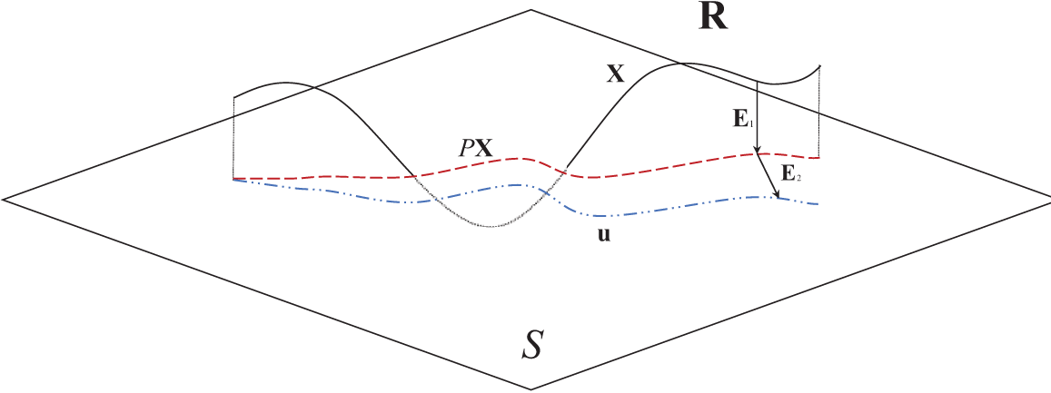
Method I: Let E(t)=uPOD(t)−X(t) denote the difference between the reduced-order solution vectors and the finite element ones. Then, we decompose the error into E(t)=E1(t)+E2(t), in which E1(t) represents the error vertical to the POD subspace while E2(t) stands for the error parallel to the POD subspace [33,34], as shown in Fig. 4.

Figure 4: Sketch of POD errors
Let P=ΨΨT∈RJ×J represent the projection matrix onto the POD subspace S, so we have
E1(t)=PX(t)−X(t),E2(t)=uPOD(t)−PX(t),
and, clearly, PX(t)∈S. Due to the orthogonality of the projection matrix, one can obtain
PE1(t)=PPX(t)−PX(t)=ΨΨTΨΨX(t)−PX(t)=PX(t)−PX(t)=0,
and
PE2(t)=PuPOD(t)−P2X(t)=ΨΨT(Ψa(t)+ups(t))−PX(t)=Ψa(t)+ups(t)−PX(t)=uPOD(t)−PX(t):=E2(t),
which further explains the meaning of the errors E1(t) and E2(t).
By the definition of the errors, we observe that the error E1(t) stems from the subspace approximation, which is only the difference between the solution and its projection onto the POD subspace and is just the POD subspace error in Eq. (22), while E2(t) is from solving the numerical model. In other words, if we only perform a low-dimensional approximation on the original vector field, the resulting error consists solely of E1(t). In this case, the total square error is given by
‖E(t)‖2=‖E1(t)‖2:=∑j=m+1kσj2,0<t≤tk,(35)
Noting that uh(t)=ϕ⋅X(t), um(t)=ϕ⋅uPOD(t) and ‖ϕ‖L2(Ω′)≤C, we have
‖uh(t)−um(t)‖L2(Ω′)≤C‖uPOD(t)−X(t)‖=C‖E(t)‖=C∑j=m+1kσj2.(36)
If the POD technique is further applied to model reduction, it will give rise to additional model errors E2(t) for t>tk. Then, we analyze the relationship between the two types of errors. The system of the linear Eq. (13) can be rewritten as
{dX(t)dt=M−1b(t)−M−1AX(t),t∈(tk,T],X(0)=[u0(x1),u0(x2),⋯,u0(xJ)]T.
Combining Eq. (23), the equivalent high-dimensional form of the system (26) can be represented as
{duPOD(t)dt=PM−1b(t)−PM−1AuPOD(t),t∈(tk,T],uPOD(tk)=PXk.
Denoting f(X(t),t)=M−1b(t)−M−1AX(t), and then taking the time derivative of both sides of E1(t)+E2(t)=uPOD(t)−X(t), we obtain
dE1(t)dt+dE2(t)dt=Pf(uPOD(t),t)−f(X(t),t),
Then, multiplying both sides of the above equation system by the projection matrix P and using the property P2=P leads to an ordinary differential equation system about the error E2(t)
{dE2(t)dt=P[f(X(t)+E1(t)+E2(t),t)−f(X(t),t)],t∈(tk,T],E2(tk)=0,(37)
where we have substituted uPOD(t) with X(t)+E1(t)+E2(t).
Let α>0 be the Lipschitz constant of the function f concerning X(t) along the direction parallel to the POD subspace, and β>0 be the Lipschitz constant in the direction perpendicular to the POD subspace. Then, for any X1(t), X2(t) located in a neighborhood of X(t) containing uPOD(t), we have
‖f(X1(t),t)−f(X2(t),t)‖≤α‖v(t)‖+β‖w(t)‖,(38)
where v(t)=P(X1(t)−X2(t)) and w(t)=X1(t)−X2(t)−v(t). Since X1(t)−X2(t)∈RJ, we have v(t)∈Rm denoting the part of X1(t)−X2(t) parallel to the POD subspace, and w(t)∈RJ−m representing the part vertical to the subspace. Due to the properties ‖P‖=‖P2‖≤‖P‖2 and ‖P‖=‖ΨΨT‖≤‖Ψ‖‖ΨT‖, we can get ‖P‖=1. From (37) and (38), we obtain
‖dE1(t)dt‖≤α‖E2(t)‖+β‖E1(t)‖.(39)
By Gronwall’s lemma [36] and E2(tk)=0, we can obtain that
‖E2(t)‖≤β∫tktexp[α(t−τ)]‖E1(τ)‖dτ,t>tk.
According to the Cauchy-Schwarz inequality, we have
‖E2(t)‖≤β(∫tktexp[2α(t−τ)]dτ)1/2(∫tkt‖E1(τ)‖2dτ)1/2≤β2αexp[2α(t−tk)]−1∑j=m+1kσj2≤β2αexp[2α(t−tk)]∑j=m+1kσj2=β2αexp[α(t−tk)]∑j=m+1kσj2,t>tk.(40)
Further information can also be obtained, i.e.,
maxtk≤t≤T‖E2(t)‖≤β2αexp[α(T−tk)]∑j=m+1kσj2.
Finally, combining (35) and (40), we get
‖E(t)‖2≤‖E1(t)‖2+‖E2(t)‖2≤∑j=m+1kσj2+β22αexp[2α(t−tk)]∑j=m+1kσj2=∑j=m+1kσj2(β22αexp[2α(t−tk)]+1),
so that
‖uPOD(t)−X(t)‖:=‖E(t)‖≤∑j=m+1kσj2(β22αexp[2α(t−tk)]+1)1/2,t>tk,(41)
which follows that
‖uh(t)−um(t)‖L2(Ω′)≤C‖uPOD(t)−X(t)‖≤C∑j=m+1kσj2(β22αexp[2α(t−tk)]+1)1/2,(42)
where C is a positive constant independent of h. If the Crank-Nicolson scheme is used for time discretization, combining (36), (42), Lemma 3.1, and the triangle inequality, we have that
‖u(tn)−umn‖L2(Ω′)≤‖u(tn)−uhn‖L2(Ω′)+‖uhn−umn‖L2(Ω′)≤{C1(h2+Δt2)+C2∑j=m+1kσj2,1≤n≤k,C1(h2+Δt2)+C2∑j=m+1kσj2(β22αexp[2α(t−tk)]+1)1/2,k+1≤n≤N,
where C1 and C2 are positive constants independent of h and Δt. To summarize, we have the following result about the convergence for the reduced-order solutions.
Theorem 4.2. If the solution u of the nonlocal diffusion equation in (2) is sufficiently smooth, and the sampling interval used to generate snapshots is given by [0,tk], we have the following error estimate for the POD reduced-order solutions {umn}n=1N
‖u(tn)−umn‖L2(Ω′)≤{C1(h2+Δt2)+C2∑j=m+1kσj2,1≤n≤k,C1(h2+Δt2)+C2∑j=m+1kσj2(β22αexp[2α(t−tk)]+1)12,k+1≤n≤N,
where C1 and C2 are positive constants independent of h and Δt.
Method II: We next present an alternative method to estimate the errors of the reduced-order solutions. Differing from the above method, we now use the following matrix approaches based on the fully discrete format.
For 1≤n≤k, given that the POD basis vectors Ψ=[ψ1,ψ2,⋯,ψm] and the modified snapshot set S=[u1,u2,⋯,uk], from Eq. (22), we have
‖S−ΨΨTS‖:=ε=∑j=m+1kσj2.
By the properties of Ψ and unps, i.e., ΨΨTunps=0, there are
uPODn=ΨΨTXn+unps=ΨΨT(Xn−unps)+unps,
It follows that
‖Xn−uPODn‖=‖(Xn−unps)−ΨΨT(Xn−unps)‖=‖un−ΨΨTun‖=‖(S−ΨΨTS)δn‖≤‖S−ΨΨTS‖‖δn‖=∑j=m+1kσj2,
where δn,n=1,2,⋯,k denote the k-dimensional identity vectors. We then obtain that
‖uhn−umn‖L2(Ω′)=‖ϕ⋅(Xn−uPODn)‖L2(Ω′)≤‖ϕ‖L2(Ω′)‖Xn−uPODn‖≤C1∑j=m+1kσj2.(43)
where ϕ=[ϕ1,ϕ2,⋯,ϕJ] denote the finite element basis functions.
When k+1≤n≤N, we set En=Xn−uPODn. Specifically, the Crank-Nicolson scheme of the finite element model can be expressed as
Xn−Xn−1+Δt2M−1AXn+Δt2M−1AXn−1=Δt2M−1(bn+bn−1).(44)
Similarly, the Crank-Nicolson scheme of the reduced-order model is denoted as
uPODn−uPODn−1+Δt2M−1AuPODn+Δt2M−1AuPODn−1=Δt2M−1(bn+bn−1).(45)
From Eqs. (44) and (45), we obtain
En−En−1+Δt2M−1AEn+Δt2M−1AEn−1=0.
Summing over k+1,⋯,n(n>k+1) for the above equations, we get that
En=Ek−ΔtM−1A∑j=k+1n−1Ej−Δt2M−1A(Ek+En),n=k+1,⋯,N,
which leads to
‖En‖≤‖Ek‖+Δt‖M−1A‖∑j=k+1n−1‖Ej‖+Δt2‖M−1A‖‖Ek‖+Δt2‖M−1A‖‖En‖,
and therefore
(1+Δt2‖M−1A‖)‖En‖≤(1+Δt2‖M−1A‖)‖Ek‖+Δt‖M−1A‖∑j=k+1n‖Ej‖,
Because
‖Ek‖=‖Xk−uPODk‖=‖(Xk−ukps)−ΨΨT(Xk−ukps)‖=‖uk−ΨΨTuk‖≤∑j=m+1kσj2,
It follows that
(1+Δt2‖M−1A‖)‖En‖≤(1+Δt2‖M−1A‖)∑j=m+1kσj2+Δt‖M−1A‖∑j=k+1n‖Ej‖≤(1+Δt2‖M−1A‖)∑j=m+1kσj2+C2Δt∑j=k+1n‖Ej‖.
From the discrete Gronwall’s lemma, we have
(1+Δt2‖M−1A‖)‖En‖≤(1+Δt2‖M−1A‖)∑j=m+1kσj2exp[C2(n−k)Δt],
so that
‖Xn−uPODn‖:=‖En‖≤∑j=m+1kσj2exp[C2(n−k)Δt],k+1≤n≤N.
Consequently, we obtain that
‖uhn−umn‖L2(Ω′)≤C1‖Xn−uPODn‖≤C1∑j=m+1kσj2exp[C2(n−k)Δt]=C1∑j=m+1kσj2exp[C2(tn−tk)],k+1≤n≤N.(46)
By (43), (46), Lemma 3.1 and the triangle inequality, we have
‖u(tn)−umn‖L2(Ω′)≤‖u(tn)−uhn‖L2(Ω′)+‖uhn−umn‖L2(Ω′)≤{C1(h2+Δt2)+C2∑j=m+1kσj2,1≤n≤k,C1(h2+Δt2)+C2∑j=m+1kσj2exp[C3(tn−tk)],k+1≤n≤N,
where C1, C2 and C3 are positive constants independent of h and Δt. Thus, we can obtain the convergence result equivalent to Theorem 4.2 for the reduced-order solutions.
Theorem 4.3. If the solution u of the nonlocal diffusion problem (2) is sufficiently smooth, and {umn}n=1N are the solutions of the reduced-order method with the sampling interval used to generate snapshots [0,tk], we have the following error estimate:
‖u(tn)−umn‖L2(Ω′)≤{C1(h2+Δt2)+C2∑j=m+1kσj2,1≤n≤k,C1(h2+Δt2)+C2∑j=m+1kσj2exp[C3(tn−tk)],k+1≤n≤N,
where C1, C2 and C3 are positive constants independent of h and Δt.
Remark 2. The error factor (∑j=m+1kσj2)1/2exp[C(tn−tk)] in Theorem 4.2 and Theorem 4.3 is caused by the POD method for model reduction, which characterizes the performance of the algorithm. More importantly, it provides a criterion for determining the number of snapshots and POD bases satisfying (∑j=m+1kσj2)1/2exp[C(tn−tk)]≤min{h2,Δt2}. In general, the singular values σj decrease rapidly and tend to 0, which means that only a very few modes can make the reduced-order error quite small. Furthermore, the factor can serve as a posteriori error estimate to design reliable adaptive model reduction methods where the number of snapshots and basis vectors can be adaptively adjusted.
5 Numerical Experiments
In this section, several numerical examples are used to verify the theoretical results and investigate the impact of different parameters on the performance of the POD reduced-order algorithm. For the 2D case, we set the computational domain Ω=(0,1)×(0,1), and the interaction domain Ωℐ=[−δ,1+δ]×[−δ,1+δ]∖Ω. Fig. 5 shows the computational domain and uniform triangulation. We choose the kernel γδ=4πδ4𝒳Bδ(x)(y) with δ=0.4, in which 𝒳Bδ(x)(y) is an indicator function. The relative L2 error and CPU elapsed time are used to measure the computational accuracy and efficiency, respectively. For finite element methods, we only record the time for solving algebraic systems, while the time consumed by the reduced-order model includes generating snapshots in the sampling interval and solving low-dimensional algebraic systems outside the sampling interval. All numerical experiments are performed on a desktop with Intel(R) Core(TM) i7-12700 2.10 GHz CPU and 32 GB of RAM, and programmed in Matlab R2016b based on Windows 11 operating system.

Figure 5: (a) The rectangular domain and (b) uniform triangulation
The error is computed by
ℰRE=‖u−uh‖L2(Ω′)‖u‖L2(Ω′)=∫Ω∪Ωℐ(u−uh)2dx∫Ω∪Ωℐu2dx=∑k=1n∫ℰk(u−uh)2dx∑k=1n∫ℰku2dx=∑k=1n∑g=1ngωgk(u(xgk)uh(xgk))2∑k=2n∑g=1ngωgku(xgk)2,(47)
where ωgk and xgk denote the quadrature weights and points in ℰk, respectively.
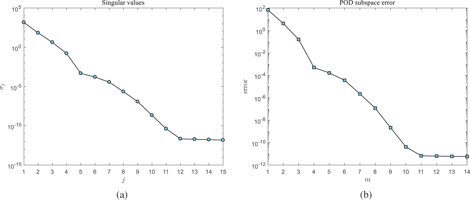
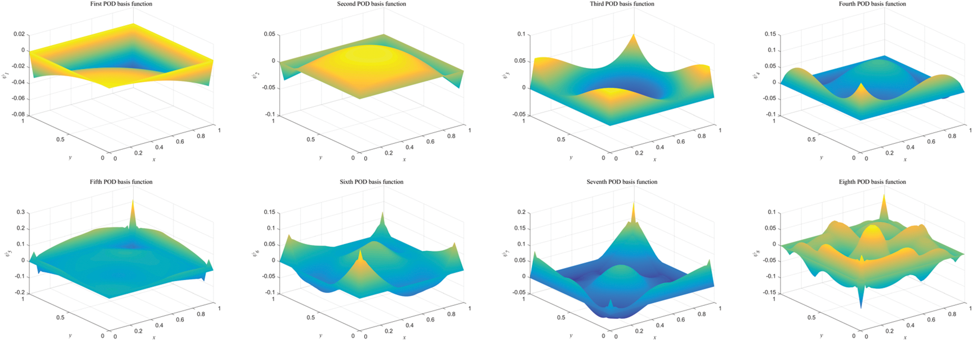
Example 1. This example examines the performance of the reduced-order algorithm. We consider a manufactured exact solution u(x,t)=(x1+t)3+(x2+t)3 with the corresponding source function f(x,t)=3(x1+t)2+3(x2+t)2−6(x1+t)−6(x2+t) and the initial condition is u0(x)=x13+x23. We take the time step as Δt=1/1000 and select a sampling interval of(0,0.5]. To ensure the optimal convergence order of the reduced-order algorithm, the subspace error ε=∑j=m+1kσj2 should be adequately small. Fig. 6a shows the distribution of singular values, and (b) shows the POD subspace errors when choosing m bases. As illustrated in Fig. 6, singular values and POD subspace errors decay rapidly and tend to zero. If Δt=10−3, there should be ε≤𝒪(10−6). From Fig. 6b, one can observe that ∑j=m+1kσj2≤10−6 when m=8, so we choose eight POD bases to construct reduced-order models, whose images are shown in Fig. 7.

Figure 6: (a) The distribution of singular values and (b) POD subspace errors with h=1/40

Figure 7: The plots of POD basis functions with h=1/40
The errors and computational time of the FEM and ROM at T=10 are listed in Table 1. One can observe from the table that the errors of the reduced-order method are nearly the same as those of the classical finite element method, while the CPU consuming time in the computations is much less than the finite element method. Besides, with the refinement of the mesh, the degrees of freedom in the finite element method increase dramatically, so the corresponding computational time increases rapidly, whereas the computational time of the ROM is much less than that of the FEM since the dimension of the ROM is extremely small (m=8). As a result, the larger the size of the algebraic systems obtained by finite element discretization, the more obvious the effectiveness of the reduced-order method.

Example 2. We test the effect of different parameters on the reduced-order algorithm to verify the theoretical results of the previous section in this example. The manufactured analytical solution is u(x,t)=(x13+x23+t2)exp(−t) with the right-hand side f(x,t)=2texp(−t)−6(x1+x2)exp(−t)−(x13+x23+t2)exp(−t) and initial condition u0(x)=x13+x23. We take h=1/10, Δt=1/1000, and m=5 with the sampling interval (0,0.05].
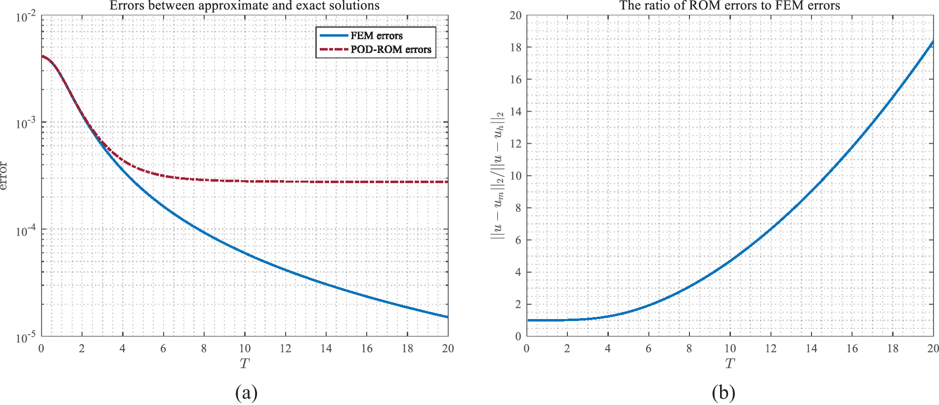
Theoretically, as time T goes on, if the snapshots and POD bases are not updated, the solutions of the POD reduced-order method will gradually fail to satisfy the accuracy requirements due to the error term (∑j=m+1kσj2)1/2exp[C(T−tk)] in Theorem 4.2 and Theorem 4.3 with fixed m and tk. To verify this hypothesis, we compare the results of the FEM and ROM. Fig. 8a shows the errors between the analytical and the finite element as well as the reduced-order solutions at different time instant T, and Fig. 8b shows the ratio of the reduced-order errors to the finite element errors, which corresponds to the error factor (∑j=m+1kσj2)1/2exp[C(T−tk)]. As seen in Fig. 8, the errors of the reduced-order solutions are larger than those of the finite element solutions with time T going on, which is caused by the POD method for model reduction to the finite element system, and cannot reach the theoretical accuracy.

Figure 8: The errors of FEM and ROM relative to analytical solutions at different time instants T
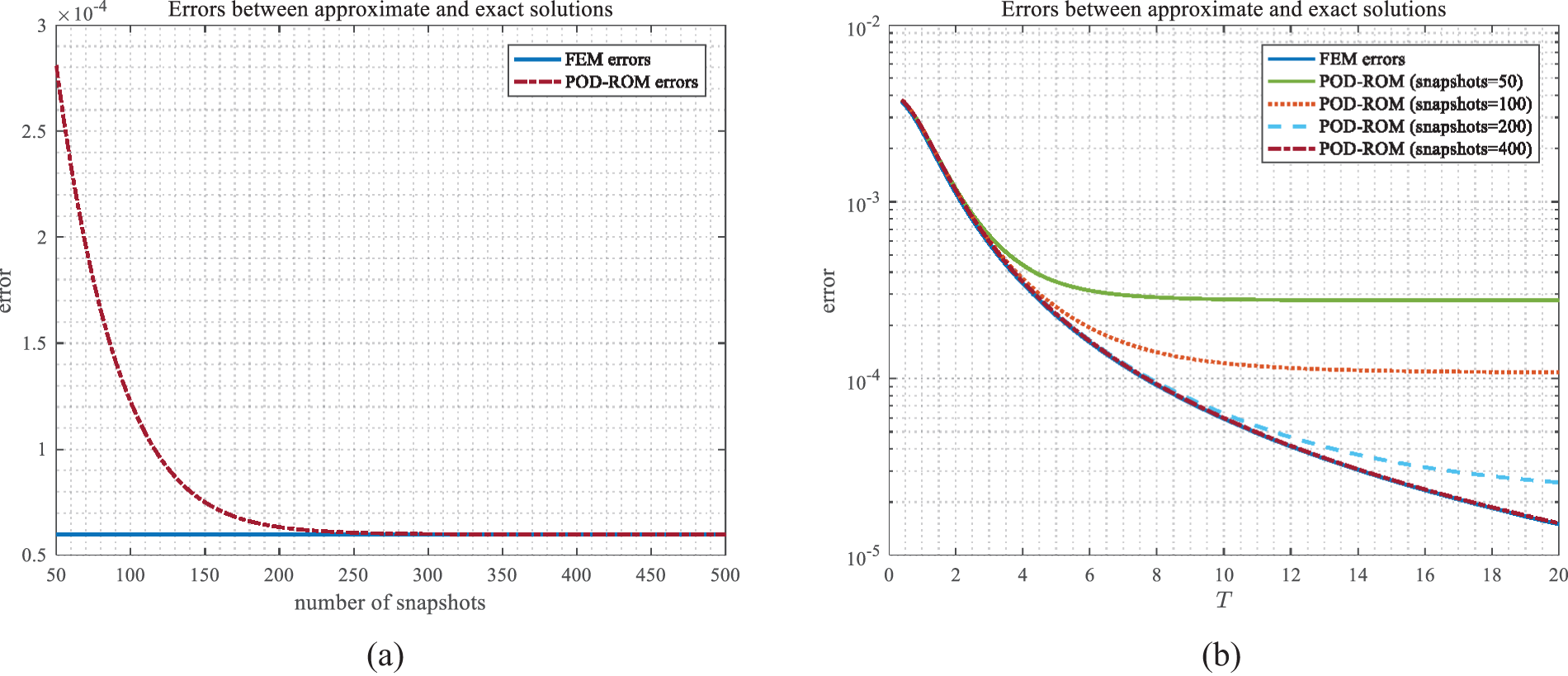
Next, we test the influences of the sampling range on the ROM. Considering that the time step is fixed, the size of the sampling range is equivalent to the number of snapshots. Fig. 9a shows the relationship between the errors of the reduced-order solutions at T=10 and the number of snapshots under the same number of POD basis vectors, in this example, m=5, where the solid blue line is the finite element error at T=10 and the red dashed line denotes the reduce-order errors. With an increasing number of snapshots, more information is incorporated into these basis vectors, which results in smaller errors. Furthermore, when the number of snapshots reaches a certain threshold, the information contained in POD bases is sufficient to compute the numerical solution accurately at the current time. As a result, the errors of the reduced-order model gradually stabilize and approach the level of the full finite element system, which is consistent with the error estimates C1(h2+Δt2)+C2∑j=m+1kσj2exp[C3(T−tk)] with fixed h, Δt, m, and T. It should be noted that increasing the number of snapshots means solving the high-dimensional finite element model more times, which will increase computational time. Fig. 9b shows the errors of the FEM and ROM at different time nodes, which also reveals that as snapshots increase, the predictive ability of the reduced-order algorithm becomes stronger.

Figure 9: (a) The relationship between the error of ROM and the number of snapshots at T=10; (b) The errors of the FEM and ROM using different number of snapshots with T increasing
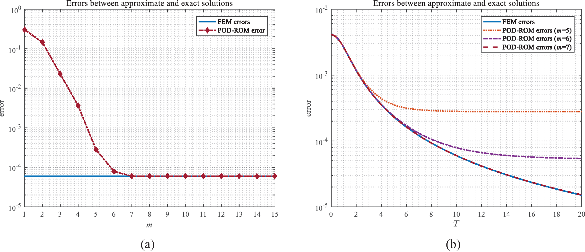
We now focus on the number of POD bases. Fig. 10a shows the relationship between the error of the reduced-order numerical solutions and the number of POD base vectors with a sampling interval (0,0.05] at T=10. As the number of basis functions increases, the reduced-order solutions exhibit a rapid reduction in error and eventually attain the precision level of the full finite element system, which indicates that only a few degrees of freedom for the reduced-order method can maintain high accuracy. In other words, the above test has implied that the singular values rapidly fall off to zero, so the error term ∑j=m+1kσj2exp[C(T−tk)] caused by model reduction with the POD method diminishes very quickly. Fig. 10b illustrates the errors of the FEM and ROM at various moments, which indicates that increasing the number of POD bases can make the ROM maintain the same level of accuracy as FEM as time T goes on.

Figure 10: (a) The relationship between the errors of ROM and the number of bases at T=10; (b) The errors of the FEM and ROM using different number of POD bases with T increasing
Example 3: In this example, we explore the impact of size parameters on the POD numerical results. Firstly, the “sampling time step” is studied, which refers to the time increment employed for calculating snapshots in the sampling interval, and can differ from the time step Δt for solving the reduced-order system outside the sampling interval. For the sake of clarity and distinction, we use Δts to represent the sample time step.
For the sake of simplicity, we consider a one-dimensional problem as follows:
{∂u∂t−2(1−s)δ2−2s∫x−δx+δu(y,t)−u(x,t)|x−y|1+2sdy=f(x,t),inΩ×(0,T],u(x,t)=(x2−x4+t2)exp(−t),inΩℐ×(0,T],u(x,0)=x2(1−x2),inΩ∪Ωℐ,(48)
where Ω=(0,1), Ωℐ=[−δ,0]∪[1,1+δ]. We take s=0 so that the source function is
f(x,t)=2texp(−t)−(x2−x4+t2)exp(−t)+(12x2−2+δ2)exp(−t),
with the exact solution u(x,t)=(x2−x4+t2)exp(−t). In this test, we set the mesh size h=1/640, the time step for solving algebraic systems Δt=1/320 as well as the interaction radius δ=0.2. We consider a fixed sampling interval (0,1] and generate several groups of snapshots with different accuracies over this interval. To achieve this, we compute several sets of finite element numerical solutions at different sampling time steps Δts in the sampling interval (0,1], and then we select several finite element solutions with an equal time interval as snapshots. By doing this, each group of snapshots contains the same number of snapshots and different groups of snapshots have different accuracies. We finally use these snapshots to generate several snapshot matrices corresponding to different sampling time steps.
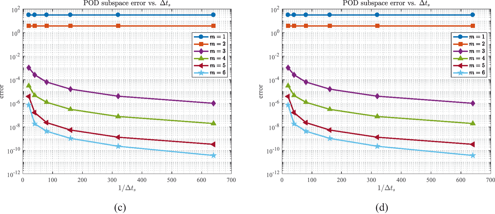
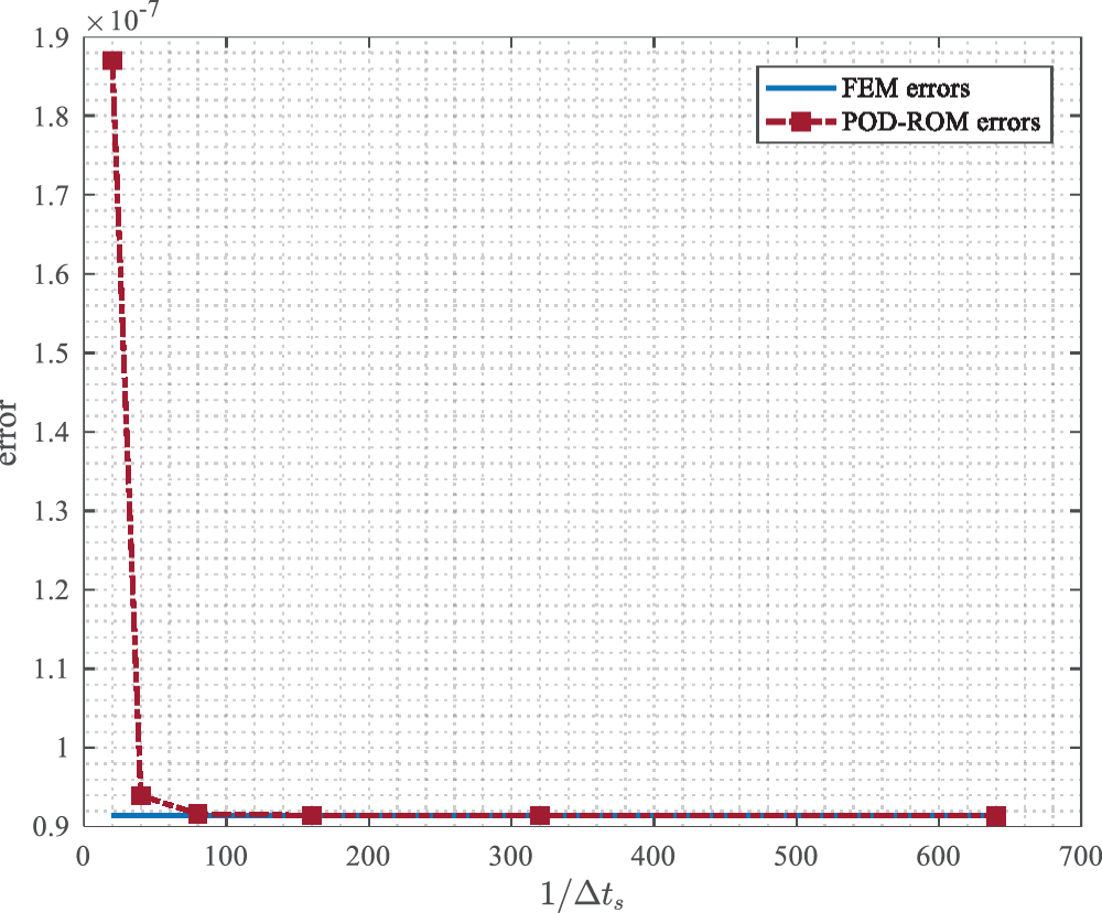
The distribution of singular values and POD subspace errors of the above generated snapshot matrices are presented by Figs. 11a and 11b. Furthermore, Figs. 11c and11d respectively indicate the relationship between the j-th singular value σj and Δts as well as the relationship between the subspace error with m POD bases and Δts, where different Δts corresponds to snapshots with varying levels of accuracy. One can visually observe that the first two dominant singular values remain relatively stable despite of different Δts, because the two singular values are foremost and contain almost all information in snapshot data, which means that they are unlikely to undergo significant changes further. For the remaining singular values, they will fall off with the refinement of Δts, because the accuracy of the snapshots improves as Δts is refined, which indicates that the same number of POD bases contains more information about snapshots and lead to the POD subspace errors ∑j=m+1kσj2 with the same number of basis vectors diminishing. From Theorem 4.2 and Theorem 4.3, the final error of the reduced-order solutions will decrease and tend to the level of the finite element system, as suggested in Fig. 12 with T=10 and m=5. Moreover, it can be also observed that when Δts>Δt, the errors of the reduced-order solutions are adequately small and almost the same as the errors of finite element solutions, which provides insights into the potential of using a larger step size Δts relative to Δt during snapshot generation to enhance computational efficiency.

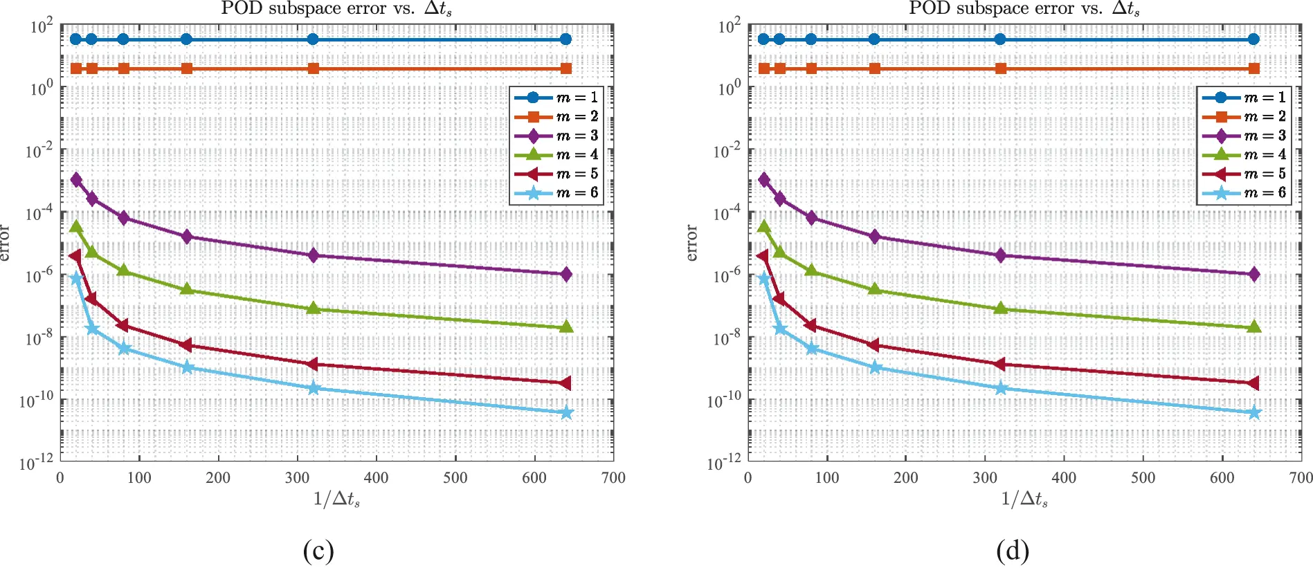
Figure 11: The distribution of (a) singular values and (b) POD subspace errors; (c) The relationship between singular values and Δts, and (d) the relationship between POD subspace errors and Δts

Figure 12: The relationship between ROM errors and sampling time steps Δts at T=10 with m=5
Below is the research about the mesh size h. We take Δts≡Δt=0.001 and the sampling interval is (0,0.1]. Taking into consideration that different h may lead to numerical solutions with different dimensions, it is meaningless to directly compare the corresponding singular value of snapshot matrices. We can obtain snapshot solution vectors with the same length by
uhn(x)=∑j=1Jhujnϕj(x),(49)
where ϕj, j=1,2,⋯,Jh are the finite element basis functions, and Jh denotes the number of finite element nodes. Specifically, for different mesh sizes h, after getting the coefficient vector [u1n,u2n,⋯,uJhn]T, we utilize (49) to calculate a series of the solution vectors {Xn}n=1k at the same set of finite element nodes, so that the snapshots for different mesh sizes have the same length. After that, we compute the relative root mean square of singular values and subspace errors by
σ~i=σi∑j=1kσj2,ε~m=∑j=m+1kσj2∑j=1kσj2,
and the relationship between the modified singular values and subspace errors with different h are shown in Fig. 13.

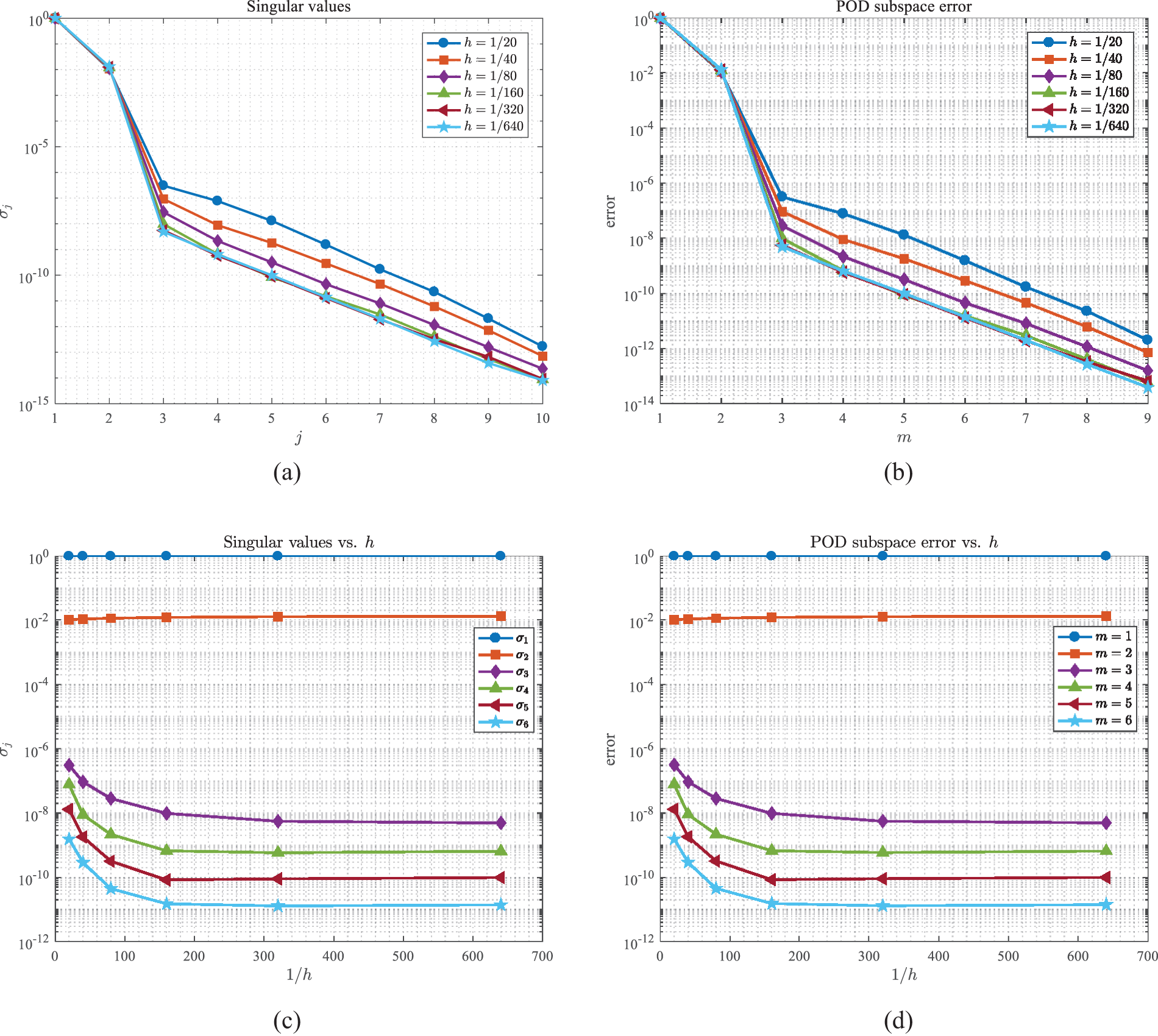
Figure 13: The distribution of (a) singular values and (b) POD subspace errors; (c) the relationship between singular values and h, and (d) the relationship between POD subspace errors and h
Similar to the situation of the sampling time step Δts, the first two dominant singular values are stable for various mesh sizes h, since they incorporate almost all information about snapshots, resulting in minimal variation of these singular values. For the remaining singular values, they decrease and eventually tend to stabilize as the mesh is refined. The above results can be easily explained as follows. The snapshots are more precise with a decrease of h, and thus, the m POD bases contain more information in snapshots so that corresponding subspace errors become smaller. Besides, the information of snapshots reaches saturation with mesh refinement. Moreover, it is worth noting that the rate of reaching saturation may also vary for different problems.
6 Conclusions
In this work, we have studied the fast reduced-order method for 2D nonlocal diffusion models based on the POD technique and Galerkin projection. The reduced-order formulation is established first, and the existence, stability as well as convergence of the reduced-order solutions are demonstrated for the nonlocal diffusion equation. In addition, we present the error estimates of the POD solutions through the utilization of two diverse methodologies. Three numerical experiments are supplied to verify the effectiveness of the algorithm and the soundness of the theoretical analysis for the nonlocal diffusion model. Importantly, we conduct a systematic analysis of how different parameters affect the performance of the reduced-order algorithm building upon the proposed theoretical and test results.
Although the reduced-order methods for nonlocal equations have been proposed, they lack a comprehensive theoretical framework. Therefore, the research undertaken in this paper is meaningful and can provide some valuable references for the development of more stable and efficient algorithms. The possibility of extending the theoretical framework to nonlinear problems and even more complex nonlocal problems, such as peridynamic equations, will be studied in future works.
Acknowledgement: The authors would like to acknowledge the support of National Natural Science Foundation of China and the Nation Key R&D Program of China.
Funding Statement: This research was supported by National Natural Science Foundation of China (No. 11971386) and the Nation Key R&D Program of China (No. 2020YFA0713603).
Author Contributions: The authors confirm contribution to the paper as follows: study conception and design: H.L. Zhang, Y.F. Nie; data collection: H.L. Zhang; analysis and interpretation of results: H.L. Zhang, Y.F. Nie; draft manuscript preparation: H.L. Zhang; paper revision: M.N. Yang, J. Wei. All authors reviewed the results and approved the final version of the manuscript.
Availability of Data and Materials: The data used to support the findings of this study are available in the manuscript.
Conflicts of Interest: The authors declare that they have no conflicts of interest to report regarding the present study.
References
1. Silling, S. (2000). Reformulation of elasticity theory for discontinuities and long-range forces. Journal of the Mechanics and Physics of Solids, 48(1), 175–209. [Google Scholar]
2. Lou, Y., Zhang, X., Osher, S., Bertozzi, A. (2010). Image recovery via nonlocal operators. Journal of Scientific Computing, 42(2), 185–197. [Google Scholar]
3. D’Elia, M., Du, Q., Gunzburger, M., Lehoucq, R. (2017). Nonlocal convection-diffusion problems on bounded domains and finite-range jump processes. Computational Methods in Applied Mathematics, 17(4), 707–722. [Google Scholar]
4. Askari, E., Bobaru, F., Lehoucq, R., Parks, M., Silling, S. et al. (2008). Peridynamics for multiscale materials modeling. Journal of Physics: Conference Series, 125, 012078. [Google Scholar]
5. Bates, P., Chmaj, A. (1999). An integrodifferential model for phase transitions: Stationary solutions in higher space dimensions. Journal of Statistical Physics, 95(5–6), 1119–1139. [Google Scholar]
6. Silling, S., Weckner, O., Askari, E., Bobaru, F. (2010). Crack nucleation in a peridynamic solid. International Journal of Fracture, 162(1–2), 219–227. [Google Scholar]
7. Silling, S., Askari, E. (2004). Peridynamic modeling of impact damage. In: Problems involving thermal hydraulics, liquid sloshing, and extreme loads on structures. San Diego, California, USA: ASMEDC. [Google Scholar]
8. Du, Q., Huang, Z., Lehoucq, R. (2014). Nonlocal convection-diffusion volume-constrained problems and jump processes. Discrete & Continuous Dynamical Systems–Series B, 19(2), 373–389. [Google Scholar]
9. Tian, H., Ju, L., Du, Q. (2015). Nonlocal convection-diffusion problems and finite element approximations. Computer Methods in Applied Mechanics and Engineering, 289, 60–78. [Google Scholar]
10. Du, Q., Gunzburger, M., Lehoucq, R., Zhou, K. (2012). Analysis and approximation of nonlocal diffusion problems with volume constraints. SIAM Review, 54(4), 667–696. https://doi.org/10.1137/110833294 [Google Scholar] [CrossRef]
11. Kunisch, K., Volkwein, S. (2001). Galerkin proper orthogonal decomposition methods for parabolic problems. Numerische Mathematik, 90(1), 117–148. [Google Scholar]
12. Kunisch, K., Volkwein, S. (2002). Galerkin proper orthogonal decomposition methods for a general equation in fluid dynamics. SIAM Journal on Numerical Analysis, 40(2), 492–515. [Google Scholar]
13. Sirovich, L. (1987). Turbulence and the dynamics of coherent structures. I. Coherent structures. Quarterly of Applied Mathematics, 45(3), 561–571. [Google Scholar]
14. Luo, Z., Chen, J., Navon, I. M., Yang, X. (2009). Mixed finite element formulation and error estimates based on proper orthogonal decomposition for the nonstationary navier-stokes equations. SIAM Journal on Numerical Analysis, 47(1), 1–19. [Google Scholar]
15. Rowley, C. W., Colonius, T., Murray, R. M. (2004). Model reduction for compressible flows using POD and Galerkin projection. Physica D: Nonlinear Phenomena, 189(1–2), 115–129. [Google Scholar]
16. Novo, J., Rubino, S. (2021). Error analysis of proper orthogonal decomposition stabilized methods for incompressible flows. SIAM Journal on Numerical Analysis, 59(1), 334–369. [Google Scholar]
17. Li, H., Wang, D., Song, Z., Zhang, F. (2021). Numerical analysis of an unconditionally energy-stable reduced-order finite element method for the Allen-Cahn phase field model. Computers and Mathematics with Applications, 96, 67–76. [Google Scholar]
18. Song, J., Rui, H. (2021). Numerical simulation for a incompressible miscible displacement problem using a reduced-order finite element method based on POD technique. Computational Geosciences, 25(6), 2093–2108. [Google Scholar]
19. Xie, D., Xu, M. (2013). A simple proper orthogonal decomposition method for von karman plate undergoing supersonic flow. Computer Modeling in Engineering & Sciences, 93(5), 377–409. [Google Scholar]
20. Narasingam, A., Siddhamshetty, P., Kwon, J. S. I. (2018). Handling spatial heterogeneity in reservoir parameters using proper orthogonal decomposition based ensemble kalman filter for model-based feedback control of hydraulic fracturing. Industrial & Engineering Chemistry Research, 57(11), 3977–3989. [Google Scholar]
21. Sidhu, H. S., Narasingam, A., Siddhamshetty, P., Kwon, J. S. I. (2018). Model order reduction of nonlinear parabolic PDE systems with moving boundaries using sparse proper orthogonal decomposition: Application to hydraulic fracturing. Computers & Chemical Engineering, 112, 92–100. [Google Scholar]
22. Witman, D., Gunzburger, M., Peterson, J. (2017). Reduced-order modeling for nonlocal diffusion problems. International Journal for Numerical Methods in Fluids, 83(3), 307–327. [Google Scholar]
23. Zhang, S., Nie, Y. (2020). A POD-based fast algorithm for the nonlocal unsteady problems. International Journal of Numerical Analysis and Modeling, 17(6), 858–871. [Google Scholar]
24. Lu, J., Nie, Y. (2022). A reduced-order fast reproducing kernel collocation method for nonlocal models with inhomogeneous volume constraints. Computers and Mathematics with Applications, 121, 52–61. [Google Scholar]
25. Du, Q., Zhou, K. (2011). Mathematical analysis for the peridynamic nonlocal continuum theory. ESAIM: Mathematical Modelling and Numerical Analysis, 45(2), 217–234. [Google Scholar]
26. Du, Q., Gunzburger, M., Lehoucq, R., Zhou, K. (2013). A nonlocal vector calculus, nonlocal volume-constrained problems, and nonlocal balance laws. Mathematical Models and Methods in Applied Sciences, 23(3), 493–540. [Google Scholar]
27. Yang, M., Nie, Y. (2023). Well-posedness and convergence analysis of a nonlocal model with singular matrix kernel. International Journal of Numerical Analysis and Modeling, 20(4), 478–496. [Google Scholar]
28. Vollmann, C. (2019). Nonlocal models with truncated interaction kernels–analysis, finite element methods and shape optimization (Ph.D. Thesis). Universität Trier, Germany. [Google Scholar]
29. D’Elia, M., Gunzburger, M., Vollmann, C. (2021). A cookbook for approximating Euclidean balls and for quadrature rules in finite element methods for nonlocal problems. Mathematical Models and Methods in Applied Sciences, 31(8), 1505–1567. [Google Scholar]
30. Lu, J., Nie, Y. (2021). A collocation method based on localized radial basis functions with reproducibility for nonlocal diffusion models. Computational and Applied Mathematics, 40(8), 1–23. https://doi.org/10.1007/s40314-021-01665-6 [Google Scholar] [CrossRef]
31. Guan, Q., Gunzburger, M. (2015). Stability and convergence of time-stepping methods for a nonlocal model for diffusion. Discrete & Continuous Dynamical Systems–Series B, 20(5), 1315–1335. [Google Scholar]
32. Gunzburger, M., Peterson, J., Shadid, J. (2007). Reduced-order modeling of time-dependent PDEs with multiple parameters in the boundary data. Computer Methods in Applied Mechanics and Engineering, 196(4–6), 1030–1047. [Google Scholar]
33. Rathinam, M., Petzold, L. (2003). A new look at proper orthogonal decomposition. SIAM Journal on Numerical Analysis, 41(5), 1893–1925. [Google Scholar]
34. Homescu, C., Petzold, L., Serban, R. (2005). Error estimation for reduced-order models of dynamical systems. SIAM Journal on Numerical Analysis, 43(4), 1693–1714. [Google Scholar]
35. Luo, Z., Chen, G. (2018). Proper orthogonal decomposition methods for partial differential equations. USA: Academic Press, Elsevier. [Google Scholar]
36. Quarteroni, A., Valli, A. (1994). Numerical approximation of partial differential equations. Berlin, Heidelberg: Springer. [Google Scholar]
 Submit a Paper
 Propose a Special lssue
 Open Access
 View Full Text
 Download PDF
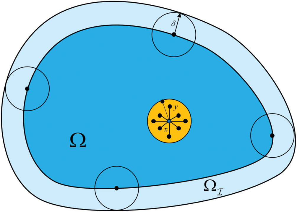


 Copyright © 2024 The Author(s). Published by Tech Science Press.
 Downloads
 Citation Tools