A Novel Framework for Learning and Classifying the Imbalanced Multi-Label Data

1  Introduction

An essential variation of typical supervised learning is known as multi-label learning. Unlike traditional supervised learning, the labels in multi-label learning are not mutually exclusive. However, it might be associated. In the case of multi-label learning, every example relates to multiple class labels concurrently [1]. Each data sample is represented predictor vector associated with multiple labels simultaneously. Let D={(xi,yj)|1≤i≤n,1≤j≤k} be the training data of—labelmulti-label, which consists of n features and k labels in the label space. Single instance (xi, yi) in a multi-label data represents an n-dimensional predictive vector (xi1,xi2,…,xin) of real values and yi is the associated k-dimensional label space (yi1,yi2,…,yik) of binary values, yij = 1 indicates label j is present in the label set of xi, else yij = 0. Given training data set D={(xi,yj)|1≤i≤n,1≤j≤k}, the multi-label learning role is to figure out a function f(.): X → 2y which predicts a correct label set y ⊆Y for a provided undetected multi-label example instance. In many real-world applications, multi-label learning is commonly used, which includes automatic image annotation [2], text categorization [3], bioinformatics [4], music categorization [5], and drug side effect prediction [6]. For the past decade, the research in multi-label learning developed various multi-label learning approaches. Still, many challenges exist in multi-learning. The number of labels for prediction, which is exponential in size, is considered a fundamental challenge to multi-label data. This involves exploiting label correlation among labels, over-fitting due to high dimensional predictive space, and highly imbalanced training sets.

Most modern existing multi-label methods try to address the first problem generally, and a couple of efforts are made to resolve the second and third issues. The performance of many standard learning algorithms is degraded due to the class imbalance problem [7]. This is the case where the classes are not present equally. The number of positive examples for each category is less than its negative counterparts. This may lead to performance degradation of the learning method. As the learning algorithms are biased to prefer the majority class, the imbalanced data can negatively affect the learning algorithms [8]. With the neglect of imbalanced class distribution, conventional state-of-the-art learning algorithms perform poorly and produce unsatisfactory suboptimal results [9,10]. The irrelevant classes can be well identified with the poor-performing learning algorithms, while the minority is reversed. The class imbalance ratio of the existing data sets used for this research has been mentioned in [11]. The use of ensemble techniques to improve accuracy in single-label classifiers has been discussed in [12]. The easiest way to handle imbalanced data is through sampling. The sampling methods are of two types: (1) under-sampling; (2) over-sampling. Random sampling leads to overfitting if the sampling ratios are not appropriately set [13]. The synthetic minority over-sampling procedure (SMOTE) makes synthetic minority cases through interpolation amongst proper training samples and k-nearest neighborhoods. Many enhancements were done over SMOTE [14–16] to improve the performance of the learning process for imbalanced binary and multi-class data.

SMOTE was adopted by [17] to handle imbalance conditions in multi-label data. First, the instances with minority labels are selected as the seed, and their nearest neighbors are identified. Next, the features of the artificial instances are created based on randomly chosen neighbors. Then the synthetic instances are created with the feature values and the label information obtained from samples with minority labels and neighbors of minority labels. This process works with the k-Nearest Neighbor (kNN) method to find the nearest neighbors for a minority label. Finally, distances are computed based on Euclidean measure, and as a result, static k numbers of neighbors are returned for a minority label. Regression is a simple but powerful statistical method to discover the linear and non-linear relationships between predictors and the response variable. Logistic Regression (LR) is a robust and computationally fast discriminative method designed to model and capture each class’s posterior probabilities. LR is a conventional statistical technique addressing binary problems. However, LR over-fits the training samples when the number of predictors vastly outstrips the number of samples. The elastic net can carry out automatic variable selection and continual contraction all at once and chooses the group of associated variables. This elastic net serves especially when the number of predictors is much larger than the variety of observations in the sample data.

Machine learning and AI methods have started to show their dominance in many fields, reference [18] showed the usage of the above two methods in the field of handwritten alphabet recognition, which plays a crucial role in pattern recognition, computer vision, and image processing. Deep Learning has been a boon in automated effective image processing. Deep learning-based automated weed in crops was presented by [19]. They used ten various rabi crops for their experimentation and proved the use of deep learning in the field. AI and deep learning-based methods could be used to handle the sheer amount of data that is being generated nowadays, and it was addressed by [20]. They managed high-dimensional data and explored their research in various application areas to justify the dominance of machine learning and deep learning. Deep learning and machine learning could also be used to address real-time social needs and have been presented by [21] to automatically detect garbage areas in remote locations.

This work addresses the imbalanced characteristic of logistic regression and the extension of logistic regression to penalized multi-label logistic regression in this paper. The adaptive weighted elastic net is used in the second phase to handle the synthetic samples produced in the first phase. This work offers an approach to make the logistic regression model work on imbalanced data. This framework introduces a new pre-processing method called Borderline MLSMOTE in phase 1. The newly created balanced multi-label dataset will combine the training dataset and generated synthetic samples. One noteworthy feature of the offered pre-processing approach is that it assists in expanding the minority labels in areas where the concurrent appearance of the minority and majority labels is too high. In the second phase, the l21-norm regularized weighted logistic regression (adaptive elastic-net) is used to handle the over-fitting and variable selection simultaneously to make the learning and prediction over the balanced data. The objectives of this research are:

•   A framework of two phases to handle and predict imbalanced multi-label data has been presented.

•   Borderline MLSMOTE has been introduced to handle difficult concurrent minority labels.

•   Adaptive weighted l21 norm regularization is presented and introduced to handle the problem of overfitting and variable selection in high-dimensional multi-label data.

•   To conduct in-depth experiments on eighteen benchmark multi-label datasets to demonstrate that the proposed framework will handle imbalanced data more effectively than existing multi-label learning techniques.

1.1 Organization of the Paper

Section 1 describes the introduction of multi-label learning, imbalanced data, logistic regression, and the paper’s contributions. Section 2 presents related works in imbalanced learning, multi-label learning, and logistic regression. Section 3 discusses the background of multi-label learning, measures for imbalance in multi-label data, a review of logistic regression, and the proposed system. Section 4 provides the speculative setup needed for the construction of the paper. Section 5 defines outcomes as well as discussion. Finally, Section 6 concludes with the end and future improvement of the work addressed in this paper.

2  Methods

Before the suggested frame was introduced, a few simple understandings regarding the methods were outlined briefly. Inside the frame, the Border MLSMOTE sampling technique is used at the pre-processing data level to resolve the imbalanced dataset by creating a synthetic dataset. Then adaptive l21-norm regularised multi-label logistic regression is used to predict the balanced multi-label data. Finally, the results show the significance of the proposed framework.

2.1 Multi-Label Learning

Let D={(xi,yj)|1≤i≤n,1≤j≤k} be the multi-label training data with p observations. The ith multi-label sample instance (xi, yi), xi is an n-dimensional predictive vector (xi1,xi2,…,xin) of real values, and yi is the associated k-dimensional label space (yi1,yi2,…,yik) of binary values. For an unseen sample x, the classifier f(.) predicts (yi1,yi2,…,yik) as a label vector for the unseen sample x. Classification whereby each example could be connected with an assortment of class labels. Each label comprises just a binary value. The multi-label classification maps an example instance to multiple labels. It is a generalization of supervised single label learning which map an example instance qi ∈ {Q} to a label set  ℓ€{£s and is given in Eq. (1).

ℏ:χ→2ℒ,i.e.,MLC(ℏ): qi ↦∏i=1kℓ where |ℓ|≥2.(1)

Problem transformation alters multi-labeled data into single labels; conventional single-label classification approaches are used on transformed data. The transformed single-labeled data are binary classifiers; conventional single-label classifiers are enough to produce the model. Adaptation in the algorithm in multi-label learning frees single-labeled classifiers to alter them to choose multi-labeled data. Thus, algorithm variation strategies are effective and free from information loss.

2.2 Measures of Imbalance in Multi-Label Data

Multi-label classification is more complex than single-label classification when addressing class imbalance. IRperLabel and MeanIR were presented by [22] to measure imbalance in multi-label data. The IRperLabel (Imbalance Rate per Label) measures each label in the dataset. It provides individual imbalance levels in the dataset. Eq. (2) shows the definition of IRperLabel:

IRperLabel =argmaxℓεL|L|(∑i=1|D|h(ℓ,Yi))∑i=1|D|h(ℓ,Yi), where h(ℓ,Yi)={1 ℓ ε Yi0 ℓ ε Yi}(2)

MeanIR represents the average imbalance in multi-label data and is shown in Eq. (3). It shows the average of IRperLabel for all labels.

MeanIR =1|L|∑i=1|L|IRperLabel(ℓi)(3)

Apart from imbalance, concurrence among the imbalanced labels also needs to be considered before balancing. Concurrence among labels represents joint appearances of relevant and irrelevant labels of the same instance. This is measured using SCUMBLE (Score of ConcUrrence among iMBalanced LabEls). It concerns the amount of imbalance variance among relevant and irrelevant labels of each instance. The concurrence measure of each instance (SCUMBLE) in the dataset is calculated, and the average of all the instances SCUMBLEi measure is given in Eqs. (4) and (5).

SCUMBLEi=1−11|D|∑i=1|D|IRperLabeli(∏i=1|D|IRperLabeli)(4)

SCUMBLE (D)=1|D|∑i=1|D|SCUMBLEi(5)

In multi-label data, a group of positive or negative labels might exist, which necessitates the algorithms to be designed in such a way as to handle a group of labels instead of a single one. Label concurrence of yeast data is depicted in Fig. 1. Arc represents labels in the dataset. The length segment of the arc describes the number of instances associated with each label. Minority labels in yeast data are class 14, class 9, class 10, and class 11; these labels appear together with one or more irrelevant labels, and these four relevant labels are difficult. Fig. 2 shows labels concurrence of emotional data. This dataset contains six labels, and the picture indicates the number of samples related to each label and interactions among labels. For example, angry-aggressive is a minority label in the emotions dataset. It appears together with other majority labels like relaxing-calm and sad-lonely.

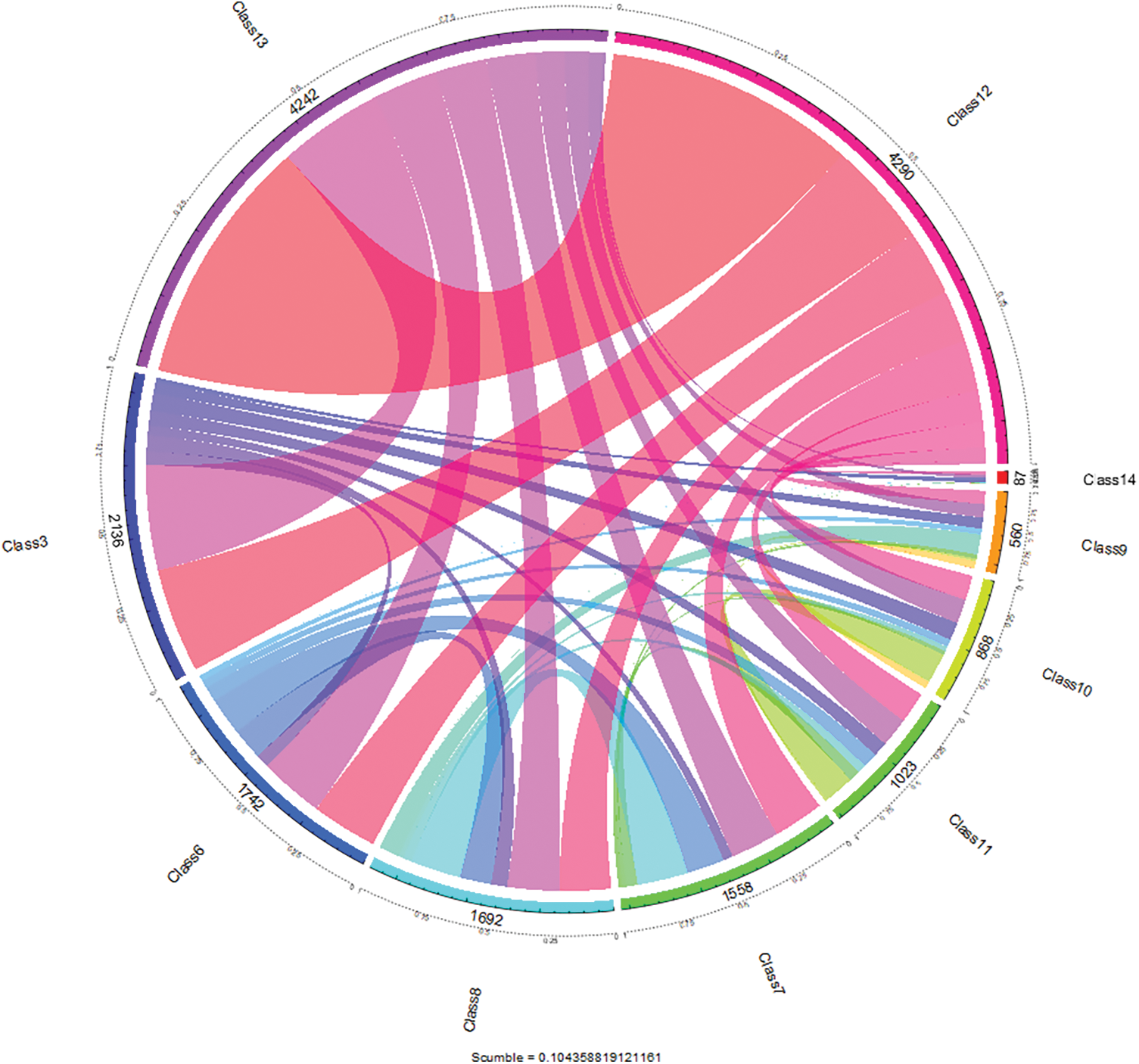
Figure 1: Label concurrence view of yeast data

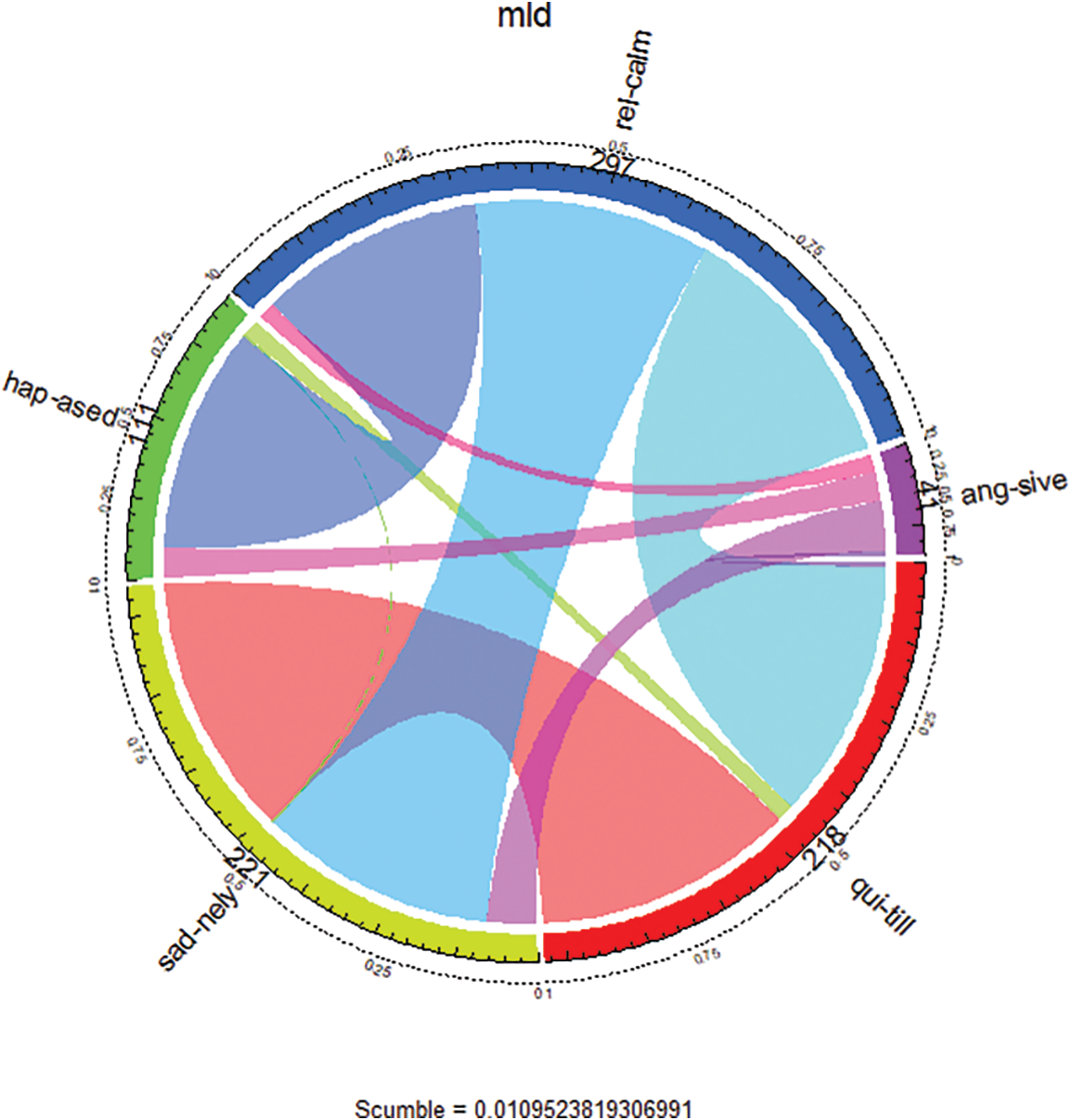
Figure 2: Label concurrence view of emotional data

2.3 Logistic Regression and Elastic Net

The logistic regression (LR) learns the relationship of predictive variables to binary 1 (“success”/“Presence”) or 0 (“failure”/“Absence”) valued response variables. When the response data is binary, logistic regression is used to find the relationship between the predictor and responses. The LR extracts some weighted predictors from predictor space and then combines them linearly. The conditional probability of LR is the joint prediction of labels in the label space given as in Eqs. (6) and (7).

pP(L|X,β)=L(Θ)=∏i=ikP(ℓi|X)(6)

=∏i=1keℓiβiTXeβiTX+e−βiTX(7)

where β=(β0,β1,…,βn) are the coefficient for the ith logistic regression to be determined and β0 is the intercept; X = (xi1, xi2, ..., xik), i = 1, 2, 3, ..., k is the input predictors of the training instances; Y = (yi1, yi2, ...., yim) is the regression object vectors, i.e., labels/targets. The predictor variables are continuous, while the response variable is binary (yes/no or present /absent). The regression coefficients are estimated using maximum likelihood estimation. The negative log-likelihood of k observations is as in Eq. (8) under the independence assumption.

P(L|X,β)=L(Θ)=−1k∑i=1k(ℓif(X′,β)+(1−ℓi)log(1−f(X′,β))(8)

To handle the ill-condition and the over-fitting problems, Eq. (8) is added with a penalty term. The penalized function of the logistic regression is given in Eq. (9). The penalty term is defined in Eq. (10).

P(L|X,β)=argminΘL(Θ)+R(Θ)(9)

L(Θ)=−1k∑i=1k[logp(ℓi|xi;β)+(1−logp(ℓi|xi;β))](10)

R(Θ)=(1+λ2m)argminβ∑i=1m‖xiβi−yi‖22+λ2∑i<m‖βi‖22+λ1∑i<m‖βi‖1(11)

R(Θ) in Eq. (11) is the elastic net regularization that learns a linear model to predict the response vector from the predictor by minimizing the squared loss with ℓ2 regularization and ℓ1 norm constraint. λ1, λ2 are the hyperparameters that decide the trade-off between the term regularization and error. These hyperparameters are the tuning parameters that provide the goodness of fit and the complexity of the model. An Elastic net is a mixture of l1 (lasso) and l2 (ridge) penalties. The lasso part of the elastic net performs variable selection, while the ridge part in the penalization stabilizes the solution paths. The amount of predictor variables exceeds the range of all samples/observations in the case of high-dimensional data analysis. When λ2 = 0, elastic net reduces to lasso. Elastic net is effective when dimensional space n is much greater than the observations p (p > n). In our research, the predictors greatly exceed the samples as they increase with the label space. Thus we choose to develop a statistical model based on the elastic net for multi-label data processing. The elastic net gives computational flexibility and performance stability.

2.4 Proposed Algorithm

CAL500, Enron, Corel5k, Rcv1 (subset1), Rcv1 (subset2), Mediamill, tmc2007, Corel6k, and eurlex-sm have SCUMBLE values more than 0.1, and they are extremely difficult MLDs. They take a high degree of concurrence amongst labels with distinct imbalance levels. Existing sampling methods ‘won’t be suitable for handling such labels with high concurrence values. On the other hand, emotions, Medical, Scene, Slashdot, Bibtex, and Genbase, have low SCUMBLE values, and the imbalanced processing with the conventional methods over these datasets will benefit. The proposed framework uses a two-stage approach to balance and predicts the imbalanced multi-label data. The first stage uses the pre-processing data to balance the imbalanced multi-label dataset. The multi-label SMOTE (MLSMOTE) implemented is modified to treat labels in the training set as a one-vs.-rest way to create new synthetic samples. Then a new balanced multi-label dataset of original and synthetic samples is given as input for adaptive weighted l21-norm regularized logistic regression to make the learning and prediction over the balanced dataset. Fig. 3 describes the flow of the data balancing approach.

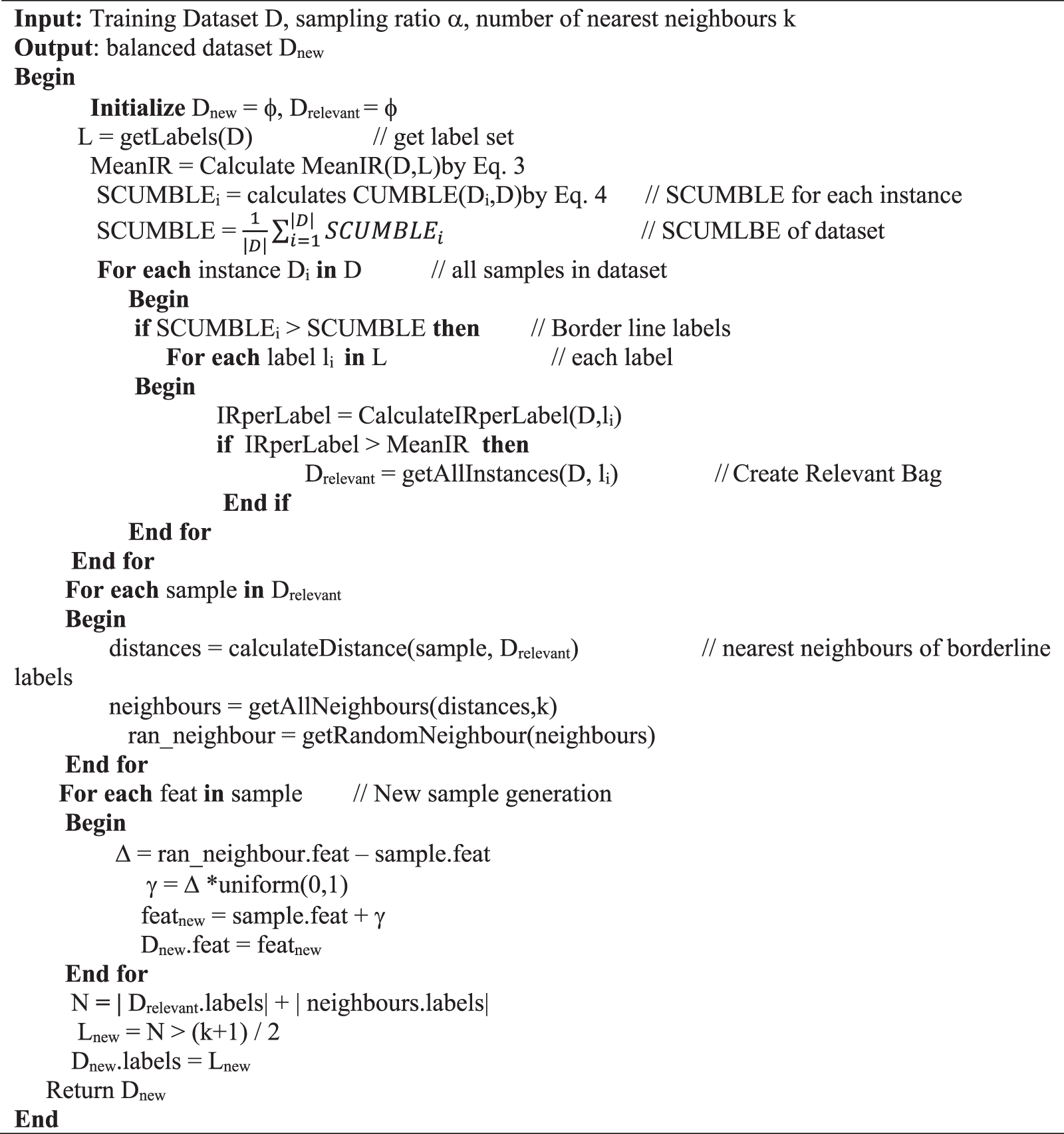
Figure 3: Phase 1-balancing the data set through Borderline-MLSMOTE

2.4.1 Borderline MLSMOTE

SMOTE system uses heuristics to pick samples with minority labels; ergo, their operation was better than other pre-processing approaches. However, to accomplish a better forecast, the sample minority labels that are high interactions with all majority labels must be obtained instead of sample majority labels. These minority labels using high concurrent values are considered borderline, and the neighboring ones tend to be more inclined to become misclassified compared to the main ones, much against the uncontrollable ones. Therefore, those concurrent minority labels tend to be more crucial for classification.

The instances with those concurrent labels tend to be somewhat more prone to become misclassified. Focusing resampling on those samples with labels that are concurrent makes it more beneficial compared to doing whole minority labels. However, the samples from the samples that are concurrent can contribute little to this classification. Our approaches are all predicated on the synthetic minority over-sampling Technique. The synthetic sample creation pre-processing creates synthetic minority samples to oversample the concurrent minority class. For each single concurrent minority label, its own k closest nearest neighbor is calculated, and then some samples are randomly chosen in line with this sampling speed. Now, the brand-new synthetic samples have been generated concerned with concurrent minority labels along with their own chosen nearest neighbor. Unlike the multi-label SMOTE system, our suggested pre-processing only reinforces the borderline (concurrent) minority samples. The generated synthetic samples are subsequently added to the unique training set. The most widely selected neighborhood size k = 5 [23] is used in this work. The flow of the proposed Borderline MLSMOTE pre-processing is shown in Fig. 3.

2.4.2 Adaptive Weighted Logistic Regression for Multi-Label Data

The adaptive weighted elastic net is used to learn and predict the balanced data set created in the first phase. The weighted regularisation ensures the handling of synthetic samples created in phase 1. The adaptive elastic-net guarantees variable selection by adding l2 regularization with an adaptive lasso to address multi-collinearity problems. Reference [24] outperformed well than an adaptive lasso and elastic–net in terms of accuracy while maintaining a higher value of true positive rate and a lower value of false negative rate with the selected predictors. The elastic net proposed in [25] is modified to an adaptive weighted elastic net via logistic regression to address three issues: over-fitting, biased estimation, multi-collinearity, and low false-positive rate. The regularization part of the elastic-net logistic regression is modified by adding weight terms to the lasso and ridge parts. The Eq. (12) is a modified adaptive elastic net.

AdaR(Θ)=(1+λ2m)argminβ∑i=1m‖xiβi−yi‖22+m2λ2∑i<mwi‖βi‖22+mλ1∑i<mwi‖βi‖1(12)

where wi > 0, i = 1, 2, ..., m are the weighted penalty coefficients. The key idea in adaptive elastic net is the weight parameter only. This weight makes the adaptive elastic net perform different amounts of shrinkage to different predictors and penalizes the smaller coefficient predictors more severely. The coefficient estimations for the elastic net are done first to construct the adaptive weights of the lasso and ridge part of the adaptive elastic net. This is presented in Eq. (13).

wi=(|βi(R(Θ))|)−γ,i=1,2…K(13)

γ is a positive constant. In this paper, we use γ = 1. The R(Θ) in Eq. (11) gives the initial estimator for weight in Eq. (13). The learning through the adaptive weighted elastic net is presented in Fig. 4. The proposed framework is illustrated in Fig. 5.

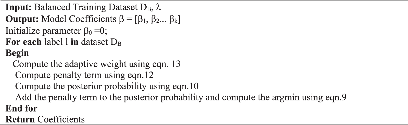
Figure 4: Phase 2-learning of balanced multi-label data through the adaptive weighted elastic net

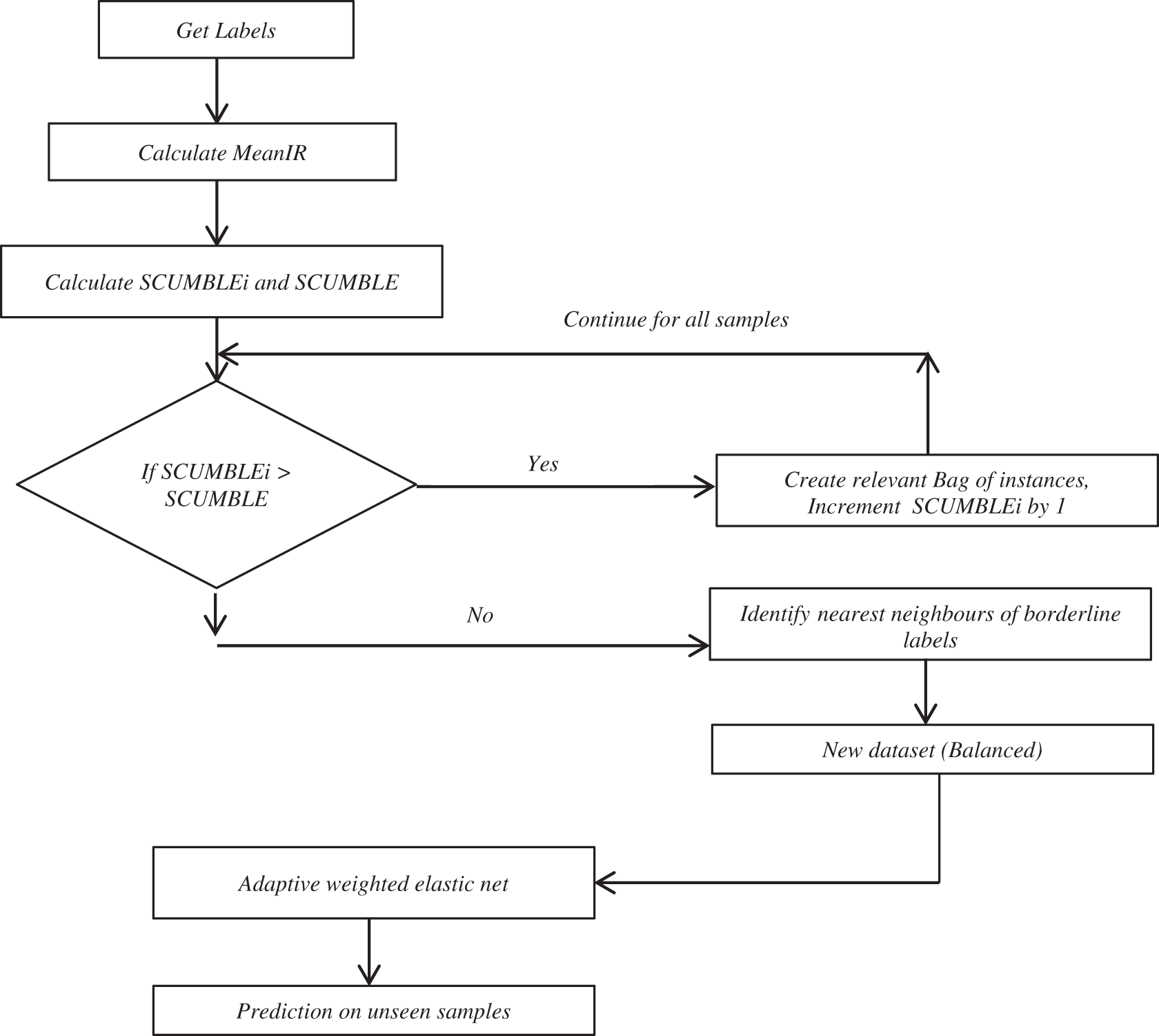
Figure 5: Proposed framework

3  Experimental Setup

This section describes the list of multi-label datasets employed with this experimentation and the evaluation metrics used to evaluate the learning algorithms.

3.1 Data Sets Used

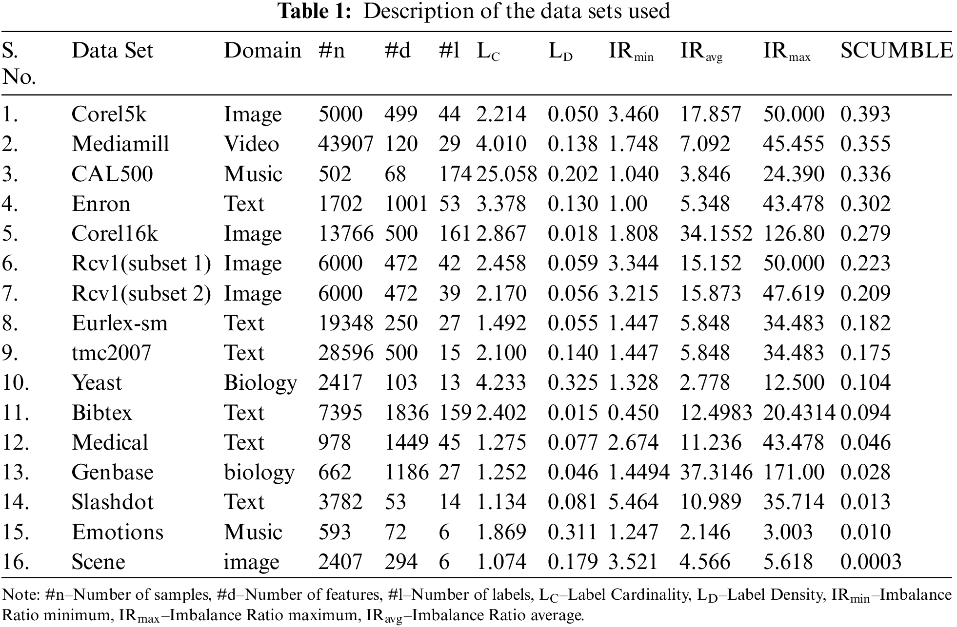
The datasets used for the experimentation are taken from various domains like music, text, image, video, and biology. All the benchmark data used here are available in the MULAN data repository. The data sets are shown in Table 1.

3.2 Evaluation Metrics

The efficiency assessment of multi-label techniques will be far more ambitious than single-label classification since it involves several labels.

1) Hamming Loss ↓ requires the error of prediction, overlooking missing errors into consideration, and testimonials the typical example-label set misclassification. Therefore, a lower h_loss value shows higher classifier performance. The hamming_Loss is specified as in Eq. (14).

h_loss(xi,yi)=1q∑i=1|q|1|ł||h(xiΔyi)|(14)

Or

Let tpi, tni, fpi and fni are the count of true positive, true negative, false positive, and false negative of ith sample, respectively, and the h_loss can be defined as in Eq. (15).

h_loss(xi,yi)=1q∑i=1|q|fpi+fnitpi+fpi+tni+fni(15)

2) One_error ↓ outlines the lack of high-positioned labels vs. the proper label in the instant collection. This step chooses the good value between 1 and 0. The smaller the value of one_error, the classifier does effectively, and it is defined as in Eq. (16).

One_error(ℏ)=1N∑i=1N‖argmaxλεℓ(xiλ)‖(16)

This step is comparable to the classification error just in a single-label classification problem.

3) Ranking Loss ↓ defines the quality of reversely ordered label sets for the specified example, plus it is also as in Eq. (17).

Ranking Loss=1N∑i=1N|λa,λb||xil||xil¯|(17)

When the ranking loss is smaller, the learning algorithm’s performance is better.

4) Average Precision ↑ computes the normal percentage of proper labels in every label set. Fundamentally, the quality has performed all applicable labels. This is provided from Eq. (18).

Average Precision=1N∑i=1N1|xil|∑λ∈xil|λ′∈xil|ri(λ) where ri(λ′)≤ri(λ)(18)

Better the significance of moderate precision improved the learning algorithm’s performance, and when standard precision = 1, the learning algorithm shows optimum performance.

5) Subset_Accuracy ↑ is characterized by the Jaccard similarity coefficient amongst label sets ℏ(xi) and yi. This step will be a type across all instances and is represented as in Eq. (19).

Subset_Accuracy(ℏ)=1N∑i=1N|ℏ(xi)∩yi||ℏ(xi)∪yi|(19)

6) Coverage ↓ is the portion of covered labels in the instance collection. Tiny the present, the higher the performance, i.e., far better label coverage. We must use the example set to cover the remaining uncovered labels if this measure is high. This is given in Eq. (20).

Cover(ℏ)=1N∑i=1Nmax_rankλεℓ(xiλ)−1(20)

4  Results and Discussion

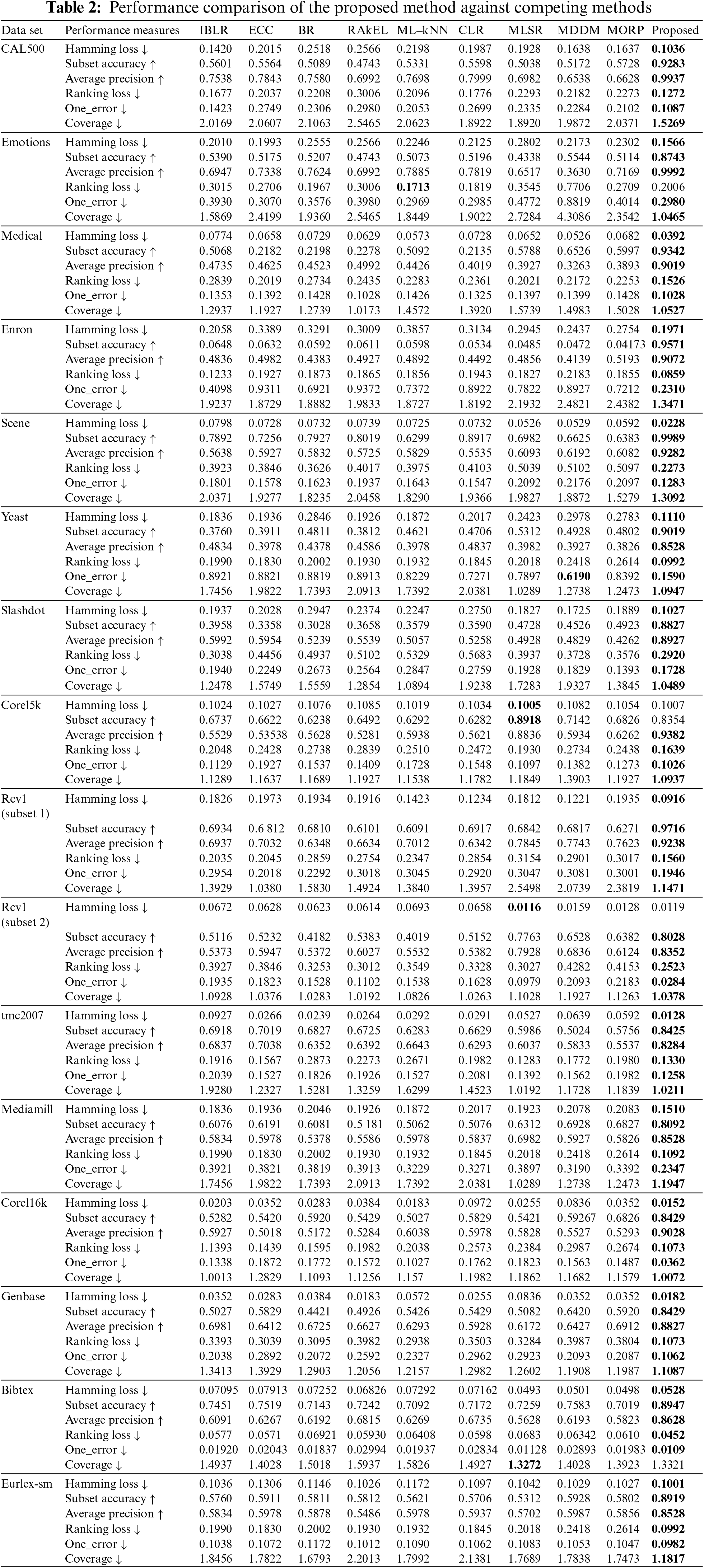
4.1 Performance Comparison of Proposed Method against Competing Methods

The performance of a multi-label classifier is assessed in the shape of several test metrics. These classification results are evaluated with five multi-label measures: Hamming Loss, Subset Accuracy, Average Precision, One Error, Ranking Loss, and Coverage. The Hamming Loss is a sample-based step that assesses the gaps between the predicted and the provided label set. Lower the Hamming, the greater the predictions. Average Precision is an example-based step and a usual performance metric. Finally, One_Error and Ranking Loss are ranking-based metrics. The different comparison methods are chosen because they have relatively high performance and efficiency.

Table 2 presents the overall performance of the proposed system. Table 2 shows that the suggested framework works quite competing methods utilized for the experimentation. The proposed method performs well on most data sets and is like other rival techniques with hamming loss and accuracy. The CAL500 exhibits 92% subset accuracy and 99% precision. The hamming loss for this dataset is 0.1. The Emotions and Medical datasets’ accuracy ranges are 87% and 93 %, respectively. The precision value on ‘Emotion’s data reaches a good 99%. In Medical data, the misclassification rate was reduced to 0.03 only. The Corel5k is a dataset with a high concurrence problem as its SCUMBLE is 0.39. Therefore, the accuracy is 83%. But for the same dataset, the MLSR produces 89% accuracy. However, the Precision is 93% with the proposed framework, and the hamming loss is 0.01. For Rcv1 (subset1) and Rcv1 (subset 2) data, the subset accuracy is 97% and 80%, respectively. The Hamming Loss measures 0.09 for Rcv1 (subset1) and 0.01 for Rcv1 (subset2). The hamming loss for Rcv1 (subset2) is much less than Rcv1 (subset1) as the SCUMBLE value of Rcv1 (subset2) is less than Rcv1 (subse1). This shows that the dataset with low concurrent value makes the learner perform well. The hamming loss for the Scene dataset is 0.02 with 99% accuracy and 92% precision value. The Scene data has a low SCUMBLE value, i.e., 0.003, among other datasets taken for our experimentation. Even though many datasets got benefited from the proposed framework, the Core5k gives the second-best Hamming Loss of 0.1007. The MLSR performs best with the Corel5k dataset, resulting in 0.1005 Hamming Loss and 89% accuracy. But still, the proposed system with Corek5k gives the second-best 83% accuracy. In general, the dataset with high concurrence labels is much benefited from the proposed system. Finally, experimentation on 17 datasets shows that the proposed framework performs better than the other nine popular methods.

4.2 Performance Comparison of Proposed Method against Recent Methods

This paper proposes a novel framework for learning and classifying the imbalanced multi-label data in two phases so that the logistic regression model will work better on imbalanced data. Phase 1 has a pre-processing method named Borderline MLSMOTE, which expands minority labels in areas where the concurrent appearance of the minority and majority labels is too high. Phase 2 has an adaptive weighted l21-norm regularized weighted logistic regression to address over-fitting and variable selection. Phase 1 uses data pre-processing to balance imbalanced multi-label data, where Multi-label SMOTE (MLSMOTE) is modified to treat labels in the training set as one-vs.-rest to create new synthetic samples. Elastic net is modified to the adaptive weighted elastic net to address over-fitting, biased estimation, multi-collinearity, and low false-positive rate. The key challenge to multi-label data lies when the number of labels for prediction is exponential. This involves exploiting label correlation among labels, over-fitting due to high dimensional predictive space, and highly imbalanced training sets. The proposed Borderline MLSMOTE is compared with other methods to demonstrate the superiority of the proposed method and is presented in Table 3. The proposed method combines two phases, and phase 2 works on pre-processed data. Most of the other comparison methods only focus on classification, which seems unfair as they work on original datasets.

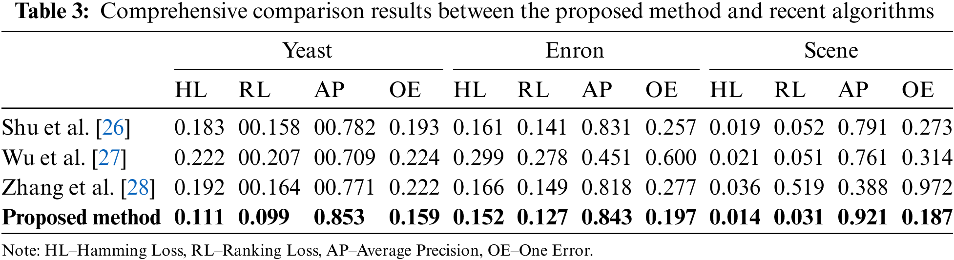
In contrast, the proposed method works on new datasets processed by Borderline MLSMOTE. Incorporating multiple cluster centers for multi-label learning (IMCC) [38] creates more samples out of neighborhood clustering centers to expand the training set and realize data enhancement. Feature-induced labeling information enrichment for multi-label learning (MLFE) [39] employs the structure information of attribute area to improve label details. Joint Ranking SVM and Binary Relevance with Robust Low-Rank Learning for Multilabel Classification (RBRL) [40] show Ranking SVM and Binary relevance with low-rank solid learning. Three standard data sets have been chosen to validate the legitimacy of the proposed method, yeast (gene function prediction using 2417 samples and 14 labels), image (image classification with 2000 samples and five labels) along with also social (5000 samples with 39 labels). The performance of the proposed framework has been examined with three recent state-of-the-art procedures and confirmed against four metrics. Table 3 shows the comparison of the proposed method against different recent works. The proposed method outperforms all metrics in yeast, image, and social dataset. The result shows the proposed method accomplishes a nearly flawless prediction on yeast, image, and social datasets and exhibits the potency of this suggested procedure.

The performance comparison of the proposed system with and without the pre-processing stage is presented in Figs. 6–8. The accuracy increases at reasonable rates for all datasets. Specifically, this framework benefited a lot of data sets with high SCUBMLE values. The datasets with high concurrent value are Corel5k, Mediamill, CAL500, Enron, Corel6k, and both Rcv1 data benefitted greatly from this framework. The accuracy of CAL500 increases to 31%, and the accuracy is 92%. With Emotions and Mediamill the percentage increase is 27.53% and 19.96%. The accuracy of Emotions is 87.43% and 80.92%. The overall increase in accuracy ranges from 7% to 31%. The overall increase in Precision for all datasets ranges from 3 % to 53%. The Corel5k dataset with high concurrence measures benefits greatly from this framework in terms of Precision—the precision value for the Corel5k dataset increases from 40% to 93%. Mediamill showed 50%; with the proposed framework, it gives 85% precision. The Scene dataset offers 87% without phase 1, which now provides 92% precision. The increase in the percentage of Precision after the framework is as follows: CAL500 (28%), Enron (37.36%), Rcv1 (Subset2) (25.14%), Eurlex-sm (24.44%), Corel6k (23.01%), tmc2007 (13.77%).

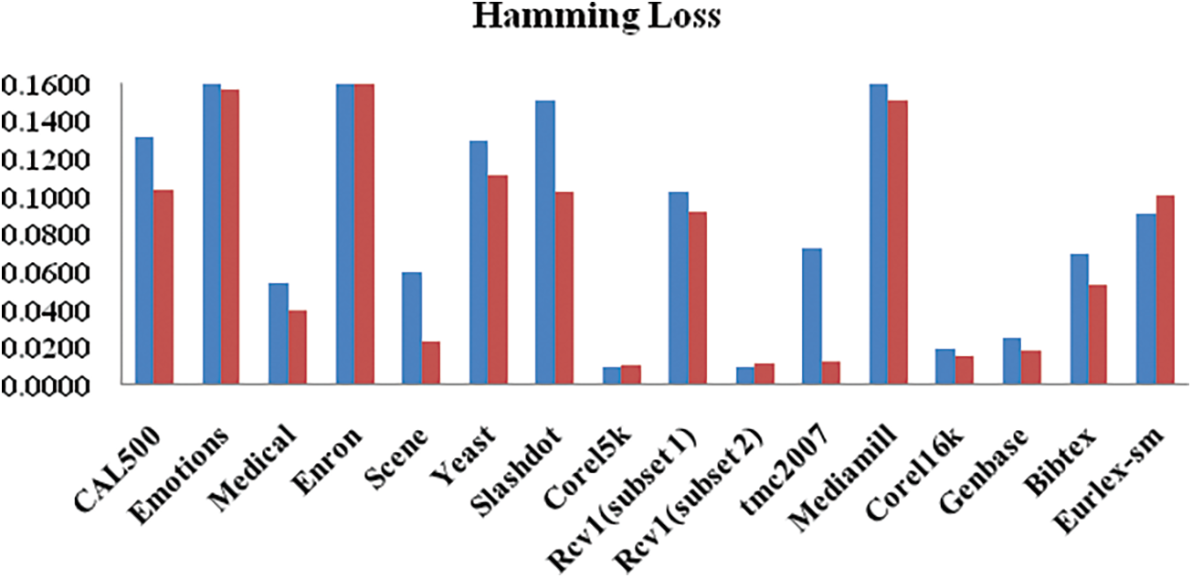
Figure 6: Hamming loss performance of adaptive weighted elastic net with and without pre-processing

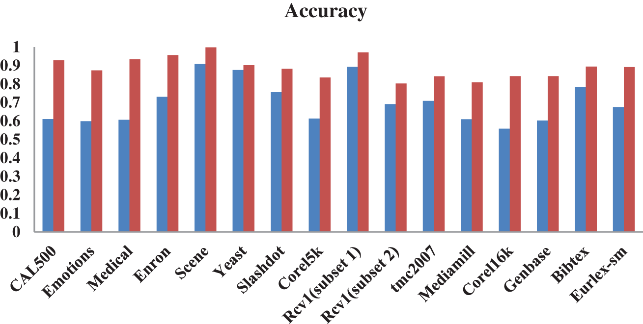
Figure 7: Accuracy of adaptive weighted elastic net with and without pre-processing

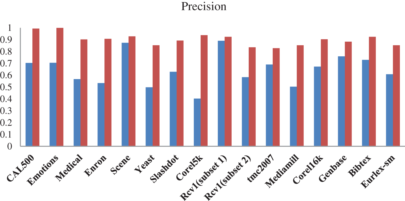
Figure 8: Performance of adaptive weighted elastic net with and without pre-processing

5  Conclusion

A framework to classify and predict imbalanced multi-label data has been introduced in this work. The framework has two phases; (1) an adaptive Borderline–MLSMOTE has proposed and pre-processed the biased data, and (2) l21-norm (Elastic net) regularized adaptive weighted logistic regression has exploited to learn parameters and predict the processed data. This variant of MLSMOTE concentrates on minority concurrence labels that contribute to the relief imbalance among multiple labels and promote the influence of minority labels. Experimental effects on various multi-label datasets have shown that the proposed framework enhances the performance over other competing and recent methods in most cases. The results confirm that the dataset with concurrent high labels benefited greatly from the proposed system. The proposed Borderline–MLSMOTE method works based on kNN to generate new samples. Identification of the k value may be challenging in Borderline–MLSMOTE. Further investigations on the imbalance of hierarchical data can be done on Borderline–MLSMOTE. The proposed sampling method is poor in identifying label correlations; additional work on the above issue could throw light on multi-label data.

Acknowledgement: This research was partly supported by the Technology Development Program of MSS (No. S3033853) and by the National Research Foundation of Korea (NRF) grant funded by the Korea government (MSIT) (No. 2021R1A4A1031509).

Funding Statement: The authors received no specific funding for this study.

Author Contributions: P. K. A. Chitra and S. Geetha contributed in conceptualization and design of the study and supervising the research process, S. Appavu alias Balamurugan and S. Geetha drafted the introduction and discussion sections, S. Geetha, Seifedine Kadry and Jungeun Kim conducted literature review and sourced relevant studies, P. K. A. Chitra and S. Geetha involved in writing the methodology section and developing research instruments, Jungeun Kim and Keejun Han conducted experiments and field work, P. K. A. Chitra and S. Geetha involved in statistical analysis and interpretation of results, P. K. A. Chitr, S. Geetha and Seifedine Kadry reviewed and edited final manuscript for submission. All authors reviewed the results and approved the final version of the manuscript.

Availability of Data and Materials: The data used in this research are open source and can be downloaded from https://mulan.sourceforge.net/datasets-mlc.html (accessed on 15 September 2022).

Conflicts of Interest: The authors declare that they have no conflicts of interest to report regarding the present study.

References

1. M. L. Zhang and Z. H. Zhou, “ML-KNN: A lazy learning approach to multi-label learning,” Pattern Recognit., vol. 40, no. 7, pp. 2038–2048, 2007. doi: 10.1016/j.patcog.2006.12.019. [Google Scholar] [CrossRef]

2. S. Feng and D. Xu, “Transductive multi-instance multi-label learning algorithm with application to automaticimage annotation,” Expert. Syst. Appl., vol. 37, no. 1, pp. 661–670, 2010. [Google Scholar]

3. Y. C. Chang, S. M. Chen, and C. J. Liau, “Multilabel text categorization based on a new linear classifier learning method and a category-sensitive refinement method,” Expert Syst. Appl., vol. 34, no. 3, pp. 1948–1953, 2008. doi: 10.1016/j.eswa.2007.02.037. [Google Scholar] [CrossRef]

4. R. M. M. Vallim, T. S. Duque, D. E. Goldberg, and A. C. Carvalho, “The multi-label OCS with a genetic algorithm for rule discovery: Implementation and first results,” in Proc. 11th Annu. Conf. Genetic Evol. Comput., 2009, pp. 1323–1330. [Google Scholar]

5. K. Trohidis, G. Tsoumakas, G. Kalliris, and I. P. Vlahavas, “Multi-label classification of music into emotions,” in Proc. 9th Int. Conf. Music Inform. Retr., 2008, vol. 8, pp. 325–330. [Google Scholar]

6. W. Zhang, F. Liu, L. Luoand, and J. Zhang, “Predicting drug side effects by multi-label learning and ensemble learning,” BMC Bioinform., vol. 16, no. 1, pp. 1–11, 2015. [Google Scholar]

7. H. He and E. A. Garcia, “Learning from imbalanced data,” IEEE Trans. Knowl. Data Eng., vol. 21, no. 9, pp. 1263–1284, 2009. [Google Scholar]

8. N. Japkowicz and S. Stephen, “The class imbalance problem: A systematic study,” Intell. Data Anal., vol. 6, no. 5, pp. 429–449, 2002. [Google Scholar]

9. R. Batuwita and V. Palade, “Class imbalance learning methods for support vector machines,” Imbalanced Learn.: Found., Algorithms, Appl., vol. 20, no. 3, pp. 83–99, 2013. [Google Scholar]

10. J. H. Xue and P. Hall, “Why does rebalancing class-unbalanced data improve AUC for linear discriminant analysis?,” IEEE Trans. Pattern Anal. Mach. Intell., vol. 37, no. 5, pp. 1109–1112, 2014. [Google Scholar]

11. M. L. Zhang, Y. K. Li, H. Yang, and X. Y. Liu, “Towards class-imbalance aware multi-label learning,” IEEE Trans. Cybern., vol. 52, no. 6, pp. 4459–4471, 2020. [Google Scholar]

12. N. V. Chawla and J. Sylvester, “Exploiting diversity in ensembles: Improving the performance on unbalanced datasets,” in Int. Workshop Multiple Classif. Syst., 2007, pp. 397–406. [Google Scholar]

13. H. Han, W. Y. Wang, and B. H. Mao, “Borderline-SMOTE: A new over-sampling method in imbalanced data sets learning,” in Int. Conf. Intell. Comput., 2005, pp. 878–887. [Google Scholar]

14. Q. Wang, Z. Luo, J. Huang, Y. Feng, and Z. Liu, “Novel ensemble method for imbalanced data learning: Bagging of extrapolation-SMOTE SVM,” Comput. Intell. Neurosci., vol. 2017, no. 3, pp. 1–11, 2017. doi: 10.1155/2017/1827016. [Google Scholar] [PubMed] [CrossRef]

15. R. C. Bhagat and S. S. Patil, “Enhanced SMOTE algorithm for classification of imbalanced big-data using random forest,” in 2015 IEEE Int. Adv. Comput. Conf. (IACC), Banglore, India, 2015, pp. 403–408. [Google Scholar]

16. Q. Gu, X. M. Wang, Z. Wu, B. Ningand, and C. S. Xin, “An improved SMOTE algorithm based on genetic algorithm for imbalanced data classification,” J. Digit. Inform. Manage., vol. 14, no. 2, pp. 92–103, 2016. [Google Scholar]

17. F. Charte, A. J. Rivera, M. J. delJesus, and F. Herrera, “MLSMOTE: Approaching imbalanced multi-label learning through synthetic instance generation,” Knowl. Based Syst., vol. 89, no. 1, pp. 385–397, 2015. doi: 10.1016/j.knosys.2015.07.019. [Google Scholar] [CrossRef]

18. R. Popli, I. Kansal, A. Garg, N. Goyal, and K. Garg, “Classification and recognition of online handwritten alphabets using machine learning methods,” IOP Conf. Series: Mat. Sci. Eng., 2021, vol. 1022, Art. no. 012111. [Google Scholar]

19. A. M. Mishra et al., “A deep learning based novel approach for weed growth estimation,” Intell. Autom. Soft Comput., vol. 31, no. 2, pp. 1157–1172, 2022. [Google Scholar]

20. S. Sharma, R. Mittal, and N. Goyal, “An assessment of machine learning and deep learning techniques with applications,” ECS Trans., vol. 107, no. 1, pp. 8979–8988, 2022. [Google Scholar]

21. V. Verma et al., “A deep learning based intelligent garbage detection system using an unmanned aerial vehicle,” Symmetry, vol. 14, no. 5, 2022, Art. no. 960. [Google Scholar]

22. F. Charte, A. Rivera, M. J. D. Jesus, and F. Herrera, “A first approach to deal with imbalance in multi-label datasets,” in Int. Conf. Hybrid Artif. Intell. Syst., 2013, pp. 150–160. [Google Scholar]

23. K. Napierala and J. Stefanowski, “Types of minority class examples and their influence on learning classifiers from imbalanced data,” J. Intell. Inform. Syst., vol. 46, no. 3, pp. 563–597, 2016. doi: 10.1007/s10844-015-0368-1. [Google Scholar] [CrossRef]

24. H. Zou and H. H. Zhang, “On the adaptive elastic-net with a diverging number of parameters,” Ann. Stat., vol. 37, no. 4, pp. 1733–1751, 2009. [Google Scholar] [PubMed]

25. H. Liu and S. Zhang, “MLSLR: Multilabel learning via sparse logistic regression,” Inf. Sci., vol. 281, no. 3, pp. 310–320, 2014. doi: 10.1016/j.ins.2014.05.013. [Google Scholar] [CrossRef]

26. S. Shu, F. Lv, Y. Yan, L. Li, S. He, and J. He, “Incorporating multiple cluster centers for multi-label learning,” Inf. Sci., vol. 590, no. 8, pp. 60–73, 2022. doi: 10.1016/j.ins.2021.12.104. [Google Scholar] [CrossRef]

27. G. Wu, R. Zheng, Y. Tian, and D. Liu, “Joint ranking SVM and binary relevance with robust low-rank learningfor multi-label classification,” Neural Netw., vol. 122, no. 3, pp. 24–39, 2020. [Google Scholar] [PubMed]

28. Q. W. Zhang, Y. Zhong, and M. L. Zhang, “Feature-induced labeling information enrichment for multi-label learning,” in Proc. AAAI Conf. Artif. Intell., 2018, vol. 32. [Google Scholar]