Path-Based Clustering Algorithm with High Scalability Using the Combined Behavior of Evolutionary Algorithms

1  Introduction

This section provides a brief overview of evolutionary algorithms and meta-heuristic optimization algorithms. A hybrid and evolutionary algorithm is utilized in this article to determine the overall optimal value during the clustering process. Then, an overview of several clustering methods used in this field and an introduction to the data clustering procedure will be followed.

In computational theory, problems can be categorized into two main classes: P and NP. The computational complexity of class P problems can be solved with a deterministic algorithm in polynomial time. Then it is relatively easy to solve. However, the complexity class of NP can be solved by a nondeterministic algorithm in polynomial time. Most real-world optimization problems and many prevalent academic problems are NP-hard. Routing and covering problems and data clustering problems are some cases of NP-hard problems [1]. For NP-Hard class problems, a provable and deterministic algorithm cannot be found in polynomial time. Therefore, using meta-heuristics and hybrid algorithms can be suitable for solving such problems.

A meta-heuristic is an iterative generation process that guides a subordinate heuristic by combining intelligently different concepts for exploring and exploiting the search space. Learning strategies structure information and find near-optimal solutions efficiently. Meta-heuristics are divided into two categories, including single-based and population-based meta-heuristics. Evolutionary algorithms are considered one type of population-based meta-heuristics.

An evolutionary algorithm (EA) uses mechanisms inspired by nature and solves problems through processes that emulate the living organism’s behaviors. EAs are inspired by the concepts in Darwinian evolution [1]. GA [2], PSO [3] and ACO [4] algorithms, widely used in solving optimization problems in different fields, are among the evolutionary algorithms proposed in the field of solving optimization problems. When addressing optimization problems, evolutionary algorithms aim to reach the optimal value more rapidly and with reduced computational complexity. Comparing the performance of Cluster Chaotic Optimization and Multimodal Cluster-Chaotic Optimization algorithms to that of eleven evolutionary optimization algorithms in the context of clustering has yielded favorable results in polynomial time [5]. However, the focus of these algorithms has been only on reaching the best general optimal value.

This paper present a hybrid population-based meta-heuristic algorithm to address the NP-Hard data clustering problem. FPC aims to achieve the general optimal value in the data clustering process while reducing the computational complexity and increasing the algorithm execution speed. The computational complexity of this algorithm is about O(k2×n).

Clustering is the process of dividing a dataset into multiple subsets that do not overlap. These subsets are called clusters. Clusters can be defined qualitatively as collections of objects within a dataset that possess higher densities within a given cluster than others [6]. Clustering is widely used in various fields, including data mining, image segmentation, computer vision, and bioinformatics. There is a wide range of clustering algorithms. Zhong et al. [7] divided these algorithms into six groups: Hierarchical Clustering, Segmentation Clustering [8], Density-based Clustering [9], grid-based clustering, model-based clustering and graph-based clustering. Clustering is an unsupervised learning issue. Unlike classification algorithms, clustering algorithms have no prior knowledge of class labels. Therefore, learning clustering is usually based on dissimilarity, directly affecting the clustering process.

In most cases, the Euclidean metric cannot measure the contrast between objects. The Minimax distance also emphasizes the connection of objects through intermediate elements relative to the mutual similarity of the elements [10]. This metric gives better clustering results when extracting arbitrary clusters in the dataset [10]. For this reason, the proposed algorithm in this paper is based on the minimax distance. The minimum spanning tree (MST) is essential in assessing complex networks’ dynamic and topological properties. This is an important component in the conversion of weighted graphs that has been addressed in several studies. A unique path in MST for the entire dataset from vertex x to vertex y is the minimax distance from x to v [11]. Therefore, minimax distance-based clustering algorithms can also be called MST-based clustering algorithms. Such algorithms begin with creating a minimum spanning tree (MST) from a given weighted graph. Subsequently, the tree is divided into different clusters by removing incompatible edges. A known problem with MST-based clustering algorithms is that they are noise-sensitive. Fischer and Buhmann proposed a path-based clustering algorithm using a cumulative optimization method based on a criterion function [10]. Their method is resistant to such noises, but their optimization method offers only a solution close to the general optimization, potentially leading to undesirable results. Finding an efficient algorithm for correctly clustering all patterns and datasets is difficult, so the clustering optimization problem is known as an NP-hard problem. By analyzing the minimax distance, we conclude that for every object x outside the C cluster, x has an equal distance to every object in the C cluster. Based on this conclusion, it can be understood that the centres of the clusters have the least density in their cluster. This theorem is one of the important components of the proposed algorithm, which will be described in Section 3. This algorithm can reach the general optimal value with computational complexity O(n2).

The rest of the paper is organized as follows: The next section briefly introduces some MST-based clustering algorithms. Section 3 describes the proposed algorithm in detail and calculates its computational complexity. Section 4 also includes experimental results of this algorithm in terms of performance and execution time, which will be compared with some of the proposed clustering algorithms. The final section will also include a summary and conclusion.

2  Related Works

The relevant research in the field of data clustering is reviewed in this section. As the paper’s topic is the presentation of a path-based clustering algorithm, this section provides an overview of path-based clustering algorithms and MST.

One of the path-based clustering methods is using the minimum spanning tree, which was first proposed by Zahn [11]. In this method, the weighted MST graph is first created from the Euclidean metric, then the incompatible edges are removed. Ideally, these edges are the longest ones in the graph. However, these assumptions are often overlooked in practice, and discarding these edges would not yield an accurate clustering. In recent years, different studies have been done to provide an efficient method for detecting incompatible edges. Furthermore, the computational complexity of the proposed method is an important issue that must be considered. Some of these algorithms have paid particular attention to their computational complexity in designing this decision tree [12]. Zhong et al. have proposed a two-step MST-based clustering algorithm to reduce the sensitivity to noise and outlier points in clustering [13]. However, this algorithm has high computational complexity and requires many parameters. Later, Zhong et al. proposed a hierarchical split-and-merger clustering algorithm [7]. In this work, MST was used in the splitting and merging process. The drawback of this algorithm is its high time complexity.

In addition to the algorithms mentioned specific algorithms also compute the dissimilarity between data pairs using MST, such as the minimax distance presented by Fischer and Buhmann [10], defined as follows:

dx,y=minp∈Px,y⁡{max1≤h<|p|⁡dp[h],p[h+1]}(1)

However, their algorithm cannot provide the global optimum value for all datasets [14]. Meanwhile, the K-means algorithm is still one of the most widely used algorithms in clustering. This is because of its efficiency, simplicity, and acceptable results in practical applications. However, K-means only works well in clustering compact and Gaussian clusters and does not work well in long clusters and those propagated in nonlinear space. The kernel K-means function was introduced to address this problem. This method plots the data in a property space of a higher dimension defined by a nonlinear function to enable linear separation of data. However, choosing a suitable function and its parameters to cluster a data set is difficult. The results of using this method have shown that spectral clustering does not have the traditional clustering algorithm’s problems, such as K-means [15]. Nevertheless, spectral clustering may present the user with many customized parameters and options, such as similarity criteria and parameters [15]. Unfortunately, the success rate of spectral clustering highly depends on these choices, which makes it difficult for the user to use this algorithm.

Chang et al. have proposed a hybrid algorithm that uses path-based and spectral clustering [16]. However, their algorithm has a significantly high computational complexity O(n3) because it requires calculating eigenvector values. One algorithm that uses minimax distance is the K-medoid algorithm, an efficient and straightforward algorithm for optimizing the criteria function. However, this algorithm may converge to the local optimum value due to its dependence on the initial values.

Ester et al. proposed a density-based clustering algorithm (DBSCAN) [9]. This algorithm requires two input values and can detect clusters of arbitrary shapes. This algorithm can cluster the dataset with the time complexity O(n2). Nonetheless, requiring the user to specify two input parameters makes it exceedingly challenging to locate suitable values for those parameters in specific datasets.

Rodriquez et al. presented an algorithm called FDPC that can cluster data with the time complexity of O(n2) [17]. It intends to find the clusters’ centres based on point density. Thus, points with a high density and a considerable distance from neighbouring points and points with a higher density than adjacent points may qualify as cluster heads. The algorithm operates on a clustering distance, denoted as dc, as input. Unpredictable distribution datasets cannot be clustered using the FDPC; it can only detect clusters with obvious cluster centres.

Normalized Cut Spectral Clustering (NCut) is one of the clustering algorithms that perform well in some types of clusters, including non-spherical and elongated clusters [18]. The accuracy of this method depends on the dependency matrix [19]. Most spectral clustering algorithms use the Gaussian kernel function as a similarity estimation method. Given this consideration, the user might encounter challenges in determining the most advantageous value of σ for the Gaussian kernel function.

One of the fastest clustering algorithms based on the minimum spanning tree is the FAST-MST algorithm, which has a time complexity of O(n3/2log⁡(n)). Due to the algorithm’s extreme noise sensitivity, points significantly distant from other points are treated as separate clusters. This problem is one of the most well-known problems in MST-based clustering algorithms.

One of the path-based clustering algorithms is the IPC algorithm. This algorithm uses Euclidean distance, minimum spanning tree, and minimax distance to extract the distance feature between elements to obtain the global optimum value with the time complexity of O(n2). Another path-based clustering algorithm is the GOPC algorithm. This algorithm requires only one input parameter (number of clusters). This parameter can be entered either by the user or estimated by the algorithm. The time complexity of this algorithm is faster than O(k×n2).

In this paper, a fast path-based clustering algorithm (which is called FPC) is presented. This algorithm can achieve the global optimal value, and the primary clustering process of the algorithm has a computational complexity of O(k2×n). However, due to the complexity of the minimum distance algorithm, the total computational complexity is O(n2).

3  Proposed Method

This section will explain the structure and function of the proposed path-based clustering method. Table 1 shows the symbols used in this section. In the following, some practical theorems used in the proposed method will be stated. The cluster center is the most central object in a cluster and is defined as follows:

In(x)=∑y∈C(x)dx,y(2)

where C(x) is the cluster with center x, and In(x) is the sum of the distances of all objects y from the cluster center x. If the cluster C(m) is the cluster whose center is m, we have ∀x∈C(m)∧x≠m, which is In(m)<In(x). This expression indicates that each cluster center has a minimum value of In(x) in its cluster. However, we cannot calculate In(x) because C(x) is unknown.

Assume that there is no noise between the clusters. A unique path in MST from the xi vertex to the xj vertex is called a minimax path from xi to xj [11]. Therefore, the minimax distance between xi and xj is equal to the length of the longest edge in its minimax path. If the distance between xii and xjj is long enough, we reach Conclusion 1.

Conclusion 1. For any object y outside the C cluster, y has a distance equal to any object in the C cluster. In other words:

Out(x)=∑y∉C(x)dx,y,(3)

So, for ∀x∈C(m)∧x≠m, we have Out(m)=Out(x).

Proposition 1. Given a cluster C(m) whose center is m, ∀x ∈ C(m)∧ x̸= m, we have ρ(m) < ρ(x), where

ρ(x)=∑y∈Udx,y,(4)

Proof:

ρ(x)=∑y∈Udx,y=∑y∈C(x)dx,y+∑y∉C(x)dx,y=In(x)+Out(x)

Since: In(m)<In(x)and Out(m)=Out(x) So: In(m)+Out(m)<In(x)+Out(x)ρ(m)<ρ(x)

Proposition 1 shows that the centers of the clusters have the lowest density (ρ) in their clusters. This theorem is used to update cluster centers.

Criteria Function: Assume that U={x1,x2,…,xn} is characterized by minimax distance. Clustering aims is to find a mapping ϕ:U→{c1,c2,…,ck} Such that each object x is in one of the k groups. In this method, the criteria function for the number of clusters k is defined as Eq. (4).

E(M)=min(m1,m2,…,mk)⁡∑i=1k∑x∈cidx,mi(5)

This algorithm is intended to find the set of cluster centers M=(m1,m2,…,mk) for the minimum value of E.

3.1 Method Details

The proposed algorithm for data clustering will be described in this section. Meta-heuristic methods have been utilized in this paper to solve the NP-hard optimization problem posed by the criterion function. An evolutionary algorithm is proposed in this paper; it models the behavior of two other evolutionary algorithms. By adopting this approach, the algorithm parallelizes the consideration of multiple M sets, the number of which corresponds to the number of particles specified in the algorithm. After completing an algorithm round and modifying the cluster centers, the criterion function’s values are evaluated until the most optimal value is determined. Then, during the next phase of algorithm execution, the selected M set is assumed to equal the elements of the M set containing all particles. In the selected M, the member of M with the lowest value In(mi) is replaced by a new random cluster center. This substitution is based on the value In(mi) of other cluster centers. The algorithm is run with the new M values. This process is repeated until the values of In(mi) are fully balanced and the criteria function reaches its minimum possible value. The final M set is then obtained.

3.1.1 Initialize the Values

To cluster each data set U, a few input parameters must be specified, which include the following in this method; Number of clusters (k): The user can enter this. Number of iterations (ITR): This can be determined by the user or algorithm itself. If selected by the algorithm, this value will be equal to k. Number of particles (P): This value can be either by the user or automatically determined by the algorithm. It is noteworthy to mention that this algorithm can also function with a P-value of 1 and can produce satisfactory clustering. The likelihood of its success declines in the process of execution. Therefore, it is necessary to choose the appropriate value to balance the accuracy and speed of the algorithm P. It is recommended that a value of P between 1 and ITR be selected. If the algorithm selects the value of p, it is determined based on Eq. (8).

P=min(round(ThrITR+1),max(ITR−1,2))(6)

where Thr is typically around 30, this value may vary based on the dataset’s cluster size and quantity. The ITR represents the quantity of algorithm iterations for which the minimum value is k.

In the first round of algorithm implementation, it is necessary to determine the centers of the clusters. Even though the algorithm’s evolution and self-correction capabilities prevent the need to precisely identify the cluster centers in the initial round, achieving optimal values can be accelerated by determining the relative locations of the cluster centers. This step will be described in the next section. Once the cluster centers have been determined, the algorithm will be iteratively executed in two phases. In the first phase, the cluster centers are updated. In the second phase, the value of the criteria function is determined, and the cluster centers of the subsequent round for each particle are calculated using the requirements function. This procedure will be repeated until the stipulated number of iterations has elapsed. At the conclusion, the optimum M set is determined based on the optimum value of the criteria function; the data are then classified based on these cluster centers. Finally, the identification and classification of noise and outliers will occur.

3.1.2 Initial Selection of Cluster Centers (M)

As previously stated, the evolutionary structure of this algorithm obviates the necessity for determining the precise cluster centers in the initial round. But optimal values of the criteria function can be obtained in less time, with fewer iterations and a smaller number of particles, by distributing initial cluster center values across the dataset space according to the cluster centers’ relative locations. The algorithm will only determine the appropriate number of particles and iterations if the initial cluster centers are distributed appropriately throughout the data space. Aside from that, additional particles and iterations will be required to achieve the ideal value. During initialization, the cluster centers of this algorithm are allocated to different locations in the data space according to their quantity. This distribution enables the algorithm to investigate the entire data space with fewer iterations and particles, ultimately achieving the general optimum value.

3.1.3 Update the Cluster Centers

In this phase, the distance of each point to the cluster centers is obtained. It is obtained using the prim algorithm’s minimax distance matrix. In the same way, the distance between all points is calculated. This process can be calculated through algorithms such as Prim et al. [19]. The resulting structure is referred to as the adjacency matrix. Based on the following steps, the cluster centers will then be updated utilizing the adjacency matrix:

Step1. First, the distance of all points with each object of the M is obtained.

Step2. Then, it is determined that each point is in which cluster using the following equation:

C(x)=argminmi∈M dx,mi(7)

Step3. Once all the points have been grouped into clusters, the value In(x) is computed for each point using Eq. (2). Subsequently, the cluster centers are revised utilizing the subsequent equation:

mi=argminx∈Ci In(x)(8)

3.1.4 Calculating the Value of the Criteria Function and the Best Particles

The criteria function’s value, derived from Eq. (5), must be determined once the preceding procedures have been executed individually for each particle. Several values are acquired after the value of this function has been computed about the number of particles. The particle with the lowest value is deemed optimal and is utilized in the algorithm’s subsequent iteration to determine the function’s minimum value.

GBest=minpi∈P⁡(E(M)pi)(9)

MGBest=Margminpi∈P(E(M)pi)(10)

Accordingly, the particle with the lowest value of the criteria function is selected as the best particle. M set of this particle will be chosen as the M set of all particles in the next round. In other words:

M(itr+1)p=MGBest,∀ itr∈ITR,1<itr<ITR,p∈P(11)

3.1.5 Selection of the Cluster Centers of the Next Round of the Algorithm

Once the GBest value and its M have been chosen as potential candidates for the subsequent round, adjustments must be made to this set to modify specific cluster centers for the next round. The steps are as follows: After sorting the values of ln⁡(mi), we select two cluster centers with the highest and lowest density values for correction, respectively. To reduce the value of the criteria function, achieving maximum balance in the density values of the clusters is imperative. By doing so, the value of the criteria function will be decreased to the greatest extent possible, and large values of the cluster density will be reduced. This violation may occur in certain circumstances. In these cases, the workflow is modified by updating the cluster centers and selecting GBest, and the cluster values and centers are optimized. The process of the algorithm in calculating the cluster centers in the next round of the algorithm is as follows:

Step1. First, the numbers of clusters with the highest (Cmax cluster) and lowest (Cmin cluster) cluster density values are specified.

Step2. The Cmin cluster is then deleted. In other words, the members of this cluster will join the nearest adjacent cluster.

Step3. Given that the number of cluster centers has decreased to k-1 clusters, there is a need to select another cluster center. This selection is made in the following two ways:

a) In some particles, the Cmax cluster will split into two clusters. In this way, another cluster center will be selected in this cluster. To do this, from points that are far from the center of the Cmax cluster (greater than the average point distance in that cluster), a point will be randomly selected as the cluster center. The best point will be selected as the cluster center.

b) In other particles, instead of selecting the center of the new cluster in the Cmax cluster, this selection is made in other clusters (which have a lower cluster density value than Cmax).

Once these steps have been completed, the algorithm will proceed to the repetition phase, executed for the number of “ITR” specified in the initial step. During each round of algorithm execution, the “BEST” value will be updated. After completing the steps and reaching the number of iterations of the algorithm, the best cluster centers can be obtained along with the value of the criterion function in the GUEST variable.

3.2 Algorithm Implementation

In this paper, a path-based clustering method is presented that can achieve the global optimal value. The main clustering process of this algorithm has a computational complexity of O(k2×n). However due to the complexity of the minimum distance algorithm, the total computational complexity is O(n2). The pseudocode of this algorithm can be seen in Algorithm 1, which consists of three parts:

a) The first part (line 1) is the preparation phase, which calculates the minimax distance between points. At this stage, the minimum spanning tree is created from the dataset. There are two algorithms for generating MST: Prim and Kruskal, whose time complexities are equal to 𝒪(n2) and 𝒪(llog⁡n), respectively. Here l is the number of edges and n is the number of vertices (or points) in the dataset. The graphs used in the clustering process are complete (i.e., l=n2). Given the complexity of both algorithms, the prim algorithm is selected to perform the calculations.

b) In the second part (lines 6–16) most of the calculations include dividing points in the specified clusters according to minimax distance from the cluster centers and updating them. In this part, the process is as follows: in lines 6–13, the distance of all points in the data set to the temporary cluster centers is checked, and each point is located in its nearest cluster. Line 14 updates the cluster centers using Eq. (8). Thus, a point within each cluster is designated as the cluster center if its distance from other points in that cluster is the shortest. In line 15, the cluster density is calculated using Eq. (2) for each cluster. In line 16, the function E(M) value is calculated and obtained from the following equation.

E(M)=∑mi∈MIn(mi)(12)

In the third part (lines 17–19), the calculations include determining the cluster centers for the next round of algorithm execution. In this section, the cluster center with the lowest cluster density is identified and replaced by a point in a high-density cluster as Algorithm 1.

The rest of the calculations includ repeating these operations per number of iterations. After completing these steps (line 22), the best cluster centers obtained are introduced as the algorithm’s output.

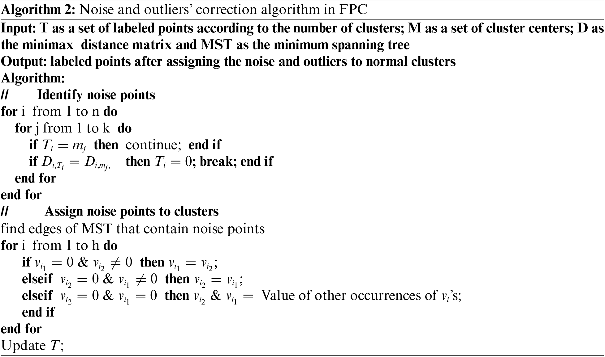
3.3 Noise and Outliers’ Problem

One of the challenges in data clustering is the management of noise and outliers. A lightweight algorithm was used in the proposed scheme to cluster these points to overcome this problem, which is explained in the following. After the final M set is obtained from the algorithm, the last step involves concatenating the noise and outliers to the nearest cluster. However, it will likely be more than one cluster with the shortest distance to a point.

In this section, the aim is to allocate these points to the nearest cluster using MST. To accomplish this, the edges of the MST are identified and placed in an independent set, ensuring that at least one of the vertices contains noise or an outlier. If both vertices of an edge contain noise and outliers, one of these two vertices must be present in another edge for that edge to include more than one vertex within the cluster. This will cluster together any noise or outliers that are close. Algorithm 2 shows the procedure of the noise and outliers’ correction and concatenation of these points to the normal clusters.

3.4 Computational Complexity

In this section, the computational complexity of the proposed algorithm will be calculated. The proposed algorithm consists of three main computational parts. The first part includes calculating the minimax distance and the adjacency matrix. The computational complexity of this part of the prim algorithm is 𝒪(n2). The calculations of the second part, which is to find the minimum minimax distance for dividing the members into clusters that require about 𝒪(k×n) calculations, then to update the cluster centers also requires about 𝒪(k×n) calculations. The second part’s calculations, which include determining the minimum minimax distance for clustering members, necessitate about 𝒪(k×n) calculations. Subsequently, updating the cluster centers also demands about 𝒪(k×n) calculations. As a result in Algorithm 2, the computational complexity of this part is about 𝒪(k×n). Given that these calculations are repeated P × ITR times, the number of ITR is equal to k by default, and the number of P using Eq. (6) is between 1 and 5. Thus, the computational complexity of this part is equal to 𝒪(k2×n)in the worst case. The computation of the cluster center determination for the next stage is performed in the third section, which possesses a computational complexity of O (k × n). Thus, the total computational complexity is as follows:

𝒪(n2)+𝒪(k2×n)+𝒪(k×n)=𝒪(n2)(13)

4  Experimental Results and Comparison with Other Algorithms

In this section, the proposed algorithm will be tested experimentally and compared with state-of-the-art algorithms in this field. Table 2 examines some of the specifications of these algorithms. The criteria of this comparison are how the data is clustered by each algorithm, the algorithm’s behaviour in clustering different datasets, the time required to perform clustering, and the computational complexity of clustering algorithms. For the sake of simplicity, the proposed algorithm is referred to as the Fast Path-based clustering algorithm (FPC) in this section.

According to Table 3, the Iris dataset consists of two scattered clusters, and the Flame consists of a spherical cluster and a semi-circular cluster. The Pathbased dataset consists of an unfinished circle and two noise clusters inside. The Spiral data set also consists of three helices. DS1 consists of three straight lines, while DS2 consists of three nested circles.

The compound comprises five clusters of different shapes and different amounts of noise. Similarly, Jain consists of two crescents with densities. D31 consists of clusters with Gaussian distribution. The Unbalance dataset is a two-dimensional dataset with 6,500 points and 8 clusters with a Gaussian distribution. The T4 has six sizes, shapes, and orientations clusters, including specific noise and random points like streaks. Aggregation also consists of seven groups of points that are perceptually divisible. The A3 dataset also consists of spherical clusters with a Gaussian distribution of 7,500 points. In all these datasets, the number of clusters is already known. Since some algorithms, such as KM, generate different results with each performance, the best results of these algorithms are compared and presented after ten iterations for each data set. The appropriate parameters for DBSCAN (EPS, MinPts) have been selected according to the algorithm proposed in [21]. Fig. 1 shows the results of clustering algorithms.

Figure 1: Results of clustering of flame (A), Spiral (B), and D31 (C) datasets using FAST-MST, RPSC, IPC, GOPC, and FPC algorithms

4.1 Comparison with MST-Based Clustering Algorithms

This subsection will examine the efficiency and clustering of the FPC algorithm and the proposed algorithms based on the minimum spanning tree. The algorithms compared to the FPC algorithm in this section include: the clustering algorithm based on a fast approximate minimum spanning tree (hereinafter referred to as FAST-MST [12]), the RPSC robust path-based spectral clustering algorithm [16], the improved path-based clustering algorithm, IPC [14], and the general optimal path-based clustering algorithm, GOPC [20]. Table 4 shows the execution times of the comparable algorithms for clustering the Flame, Spiral, and D31 datasets. Given that the Flame dataset contains 240 points and the Spiral has 312 points, these two datasets are too small to compare the time complexity of each algorithm. The D31 dataset, comprising 3100 data points, is used in this comparison.

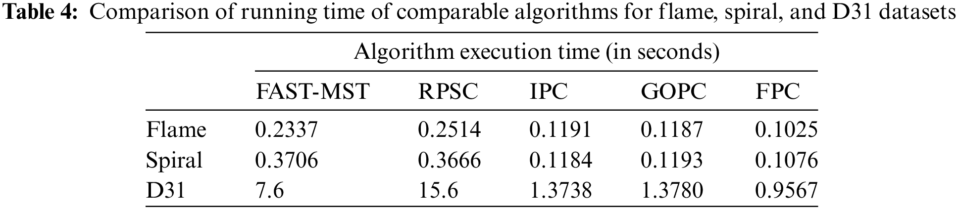
According to the results presented in Fig. 1 and Table 4, the following can be concluded:

1.    IPC, GOPC, and FPC all present the same clustering results and all three can correctly cluster datasets with different shapes.

2.    In clustering smaller datasets, all three IPC, GOPC, and FPC algorithms have approximately the same runtime (however FPC is slightly faster in this dataset).

3.    FPC operates much faster (about 50% faster) than other algorithms in clustering large data sets.

4.    RSPC also provides acceptable results in the clustering process but has a higher time complexity than IPC, GOPC, and FPC.

5.    FAST-MST is highly sensitive to noise. This is a known drawback in most MST-based clustering algorithms.

4.2 Comparison with Other Clustering Algorithms

This section compares the FPC algorithm with the clustering algorithms in this field. Figs. 2 and 3show the clustering results of the above algorithms for clustering 12 datasets with different shapes and sizes. This dataset can be seen in Table 4. Fig. 2 shows the clustering results of the first series of datasets, which are mostly small in size and limited in the number of clusters for K-means, DBSCAN, NCut, FDPC, IPC, GOPC, and FPC algorithms. According to the results, it can be seen that FPC has the best performance in terms of clustering among other algorithms.

Figure 2: Clustering results of the first series of datasets with the desired algorithms. Datasets: (A) Iris, (B) Flame, (C) Pathbased, (D) Jain, (E) DS1, (F) DS2

Figure 3: Runtime comparison of algorithms for first series datasets

Fig. 3 shows the execution times of the compared algorithms for clustering the Iris, Flame, Pathbased, Jain, DS1, and DS2 datasets. In the Fig. 3, it can be seen that FPC has a good execution time in clustering this data set. The Iris dataset is the only instance where the DBSCAN algorithm outperforms FPC in clustering. However, it should be noted that in this case, DBSCAN fails to classify the noise and treats it as an independent cluster, whereas FPC does so. FPC has nearly the same execution time as FDPC, GOPC, and IPC in most cases; however, based on the clustering method and performance metrics, it is evident that FPC outperformed the others. In Path-based dataset clustering, the execution time of the FPC algorithm is longer than FDPC, GOPC, IPC, and DBSCAN algorithms. According to Fig. 3, the DBSCAN algorithm failed to perform the clustering operation correctly. The FDPC algorithm also had a lower performance than the FPC.

Regarding GOPC and IPC, their performance is comparable, and time differences are negligible; however, these two algorithms cluster this data set marginally quicker than FPC. However, given that FPC outperforms IPC and GOPC in the majority of the previous datasets, it can be concluded that the FPC algorithm has the best performance in terms of runtime and clustering in this section when compared to other algorithms. Eq. (1), which represents the formula for determining the number of particles in FPC, demonstrates that as the number of points and size of the datasets increase, so does the speed of FPC, enabling it to perform clustering operations more rapidly. Similarly, Fig. 4 shows the results of the second series clustering of the datasets, which often have a larger size and more clusters than the first series.

Figure 4: Clustering results of the first series of datasets with the desired algorithms. Datasets: (A) Compound, (B) Aggregation, (C) D31, (D) Unbalance, (E) A3, (F) T4

According to the results, it can be seen that FPC, IPC, and GOPC have the best performance in clustering among other algorithms, except for the Aggregation dataset. Due to a narrow line connecting the two right clusters being a suitable data set, detection by MST-based algorithms and the minimax distance is challenging. The execution time of the Compound and Aggregation data clustering process for the compared algorithms can be seen in Fig. 5. Following FDPC, the FPC algorithm shows the quickest execution time in clustering the datasets illustrated in the Fig. 5, except for Aggregation, where the FDPC algorithm exhibits superior performance in terms of both clustering and execution time, the IPC, GOPC and FPC algorithms demonstrate comparable performance in these aspects while also surpassing alternative algorithms in terms of efficiency.

Figure 5: Runtime comparison of desired algorithms for compound and aggregation datasets

Fig. 6 shows the runtime clustering of D31, Unbalance, A3, and T4 datasets for the discussed algorithms. In this form, the K-means algorithm has the shortest runtime but performs worse than others. The FDPC algorithm is then faster but performs poorly as NCut in the A3 and T4 datasets. Only IPC, GOPC, and FPC algorithms perform well in clustering these datasets. Therefore, according to Fig. 6, it can be seen that FPC has a faster runtime than IPC and GOPC. IPC, GOPC, and FPC algorithms have similar clustering performances due to their similar structure. However, FPC is faster than IPC and GOPC in terms of runtime.

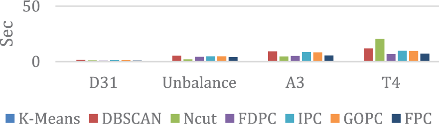
Figure 6: Runtime comparison of desired algorithms for medium-sized datasets

Based on these comparisons, it can be concluded that the proposed algorithm in this paper (FPC) in clustering the Table 4 datasets is more efficient regarding performance and execution time among the noted algorithms. The K-means algorithm also has the worst performance among the other algorithms. Despite the high speed of the clustering process, FDPC cannot adequately cluster non-Gaussian distributed datasets. This proves that the FDPC can only detect clusters that have specific centers [17]. DBSCAN can detect clusters of arbitrary shapes in most sets, but finding suitable parameters for some datasets, including Path-based, is difficult. When clustering additional datasets with DBSCAN, an approximation of the EPS value is possible, even when the algorithm described in [21] is utilized. Accurately determining both parameters requires trial and error, which causes this algorithm to be more time-consuming than others.

5  Conclusion

This paper presents FPC, an exclusive and hybrid algorithm, for optimizing and minimizing the criteria function. The FPC was compared with state-of-the-art clustering algorithms in clustering two-dimensional datasets of different shapes. In the meantime, FPC overcame other competitors in efficiency and performance and showed good performance in the clustering procedure. FPC requires three parameters k, ITR, and P that the ITR and P parameters can be calculated by the algorithm itself or entered by the user manually. So, typically, the algorithm only needs the k parameter. This makes FPC a general clustering algorithm with the same behavior in clustering different datasets. Nevertheless, this algorithm encounters a challenge when confronted with interconnected clusters. This was observed in Aggregation dataset clustering in which the FPC could not detect two interconnected clusters. This connection causes the distance between the points in that area to be less than the value required to separate the clusters. Another problem with FPC is its computational complexity, around 𝒪(n2). Despite this satisfactory value, it remains below the optimal level. The most important reason for this complexity is using the prim’s algorithm to create the MST and the minimax distance. By solving this problem, the execution speed of the algorithm can be increased up to ten times, and its computational complexity can be improved to 𝒪(k2×n). Future work to improve this algorithm can address the above problems and solutions to address them. Providing solutions to these problems can make FPC much more practical and faster.

Acknowledgement: There is no acknowledgements in this article.

Funding Statement: The authors received no specific funding for this study.

Author Contributions: The authors confirm contribution to the paper as follows: study conception and design: M. Esmaeilpour, L. Safari-Monjeghtapeh; data collection: L. Safari-Monjeghtapeh; analysis and interpretation of results: M. Esmaeilpour, L. Safari-Monjeghtapeh; draft manuscript preparation: M. Esmaeilpour, L. Safari-Monjeghtapeh. All authors reviewed the results and approved the final version of the manuscript.

Availability of Data and Materials: Data sharing is not applicable to this article as no datasets were generated or analyzed during the current study.

Conflicts of Interest: The authors declare that they have no conflicts of interest to report regarding the present study.

References

1. M. A. Ebrahimi, H. D. Dehnavi, M. Mirabi, M. T. Honari and A. Sadeghian, “Solving NP hard problems using a new genetic algorithm,” International Journal of Nonlinear Analysis and Applications, vol. 14, no. 1, pp. 275–285, 2022. [Google Scholar]

2. S. Katoch, S. S. Chauhan and V. Kumar, “A review on genetic algorithm: Past, present, and future,” Multimedia Tools Applications, vol. 80, no. 5, pp. 8091–8126, 2021 [Google Scholar] [PubMed]

3. A. G. Gad, “Particle swarm optimization algorithm and its application: A systematic review,” Archives of Computational Methods in Engineering, vol. 29, no. 5, pp. 2531–2561, 2022. [Google Scholar]

4. Z. J. Lee, S. F. Su, C. C. Huang, K. H. Liu, X. Xu et al., “Genetic algorithm with ant colony optimization (GA-ACO) for multiple sequence alignment,” Applied Soft Computing, vol. 8, no. 1, pp. 55–78, 2008. [Google Scholar]

5. J. Gálvez, E. Cuevas and K. Gopal Dhal, “A competitive memory paradigm for multimodal optimization driven by clustering and chaos,” Mathematics, vol. 8, no. 6, pp. 934–963, 2020. [Google Scholar]

6. Y. G. Fu, J. F. Ye, Z. F. Yin, Z. F. Chen, L. Wang et al., “Construction of EBRB classifier for imbalanced data based on fuzzy C-means clustering,” Knowledge-Based Systems, vol. 234, pp. 107590, 2021. [Google Scholar]

7. C. Zhong, D. Miao and P. FränKnowlti, “Minimum spanning tree based split-and-merge: A hierarchical clustering method,” Information Sciences, vol. 181, no. 16, pp. 3397–3410, 2011. [Google Scholar]

8. M. Capó, A. Pérez and J. A. Lozano, “An efficient approximation to the K-means clustering for massive data,” Knowledge-Based Systems, vol. 117, pp. 56–69, 2017. [Google Scholar]

9. M. Ester, H. P. Kriegel, J. Sander and X. Xu, “A density-based algorithm for discovering clusters in large spatial databases with noise,” in Proc. of the Second Int. Conf. on Knowledge Discovery and Data Mining, KDD-96, Portland, Oregon, AAAI Press, vol. 96, no. 34. pp. 226–231, 1996. [Google Scholar]

10. B. Fischer and J. M. Buhmann, “Path-based clustering for grouping of smooth curves and texture segmentation,” IEEE Transactions on Pattern Analysis and Machine Intelligence, vol. 25, no. 4, pp. 513–518, 2003. [Google Scholar]

11. C. T. Zahn, “Graph-theoretical methods for detecting and describing gestalt clusters,” IEEE Transactions on Computers, vol. C-20, no. 1, pp. 68–86, 1971. [Google Scholar]

12. R. Jothi, S. K. Mohanty and A. Ojha, “Fast approximate minimum spanning tree based clustering algorithm,” Neurocomputing, vol. 272, pp. 542–557, 2018. [Google Scholar]

13. C. Zhong, D. Miao and R. Wang, “A graph-theoretical clustering method based on two rounds of minimum spanning trees,” Pattern Recognition, vol. 43, no. 3, pp. 752–766, 2010. [Google Scholar]

14. Q. Liu, R. Zhang, R. Hu, G. Wang, Z. Wang et al., “An improved path-based clustering algorithm,” Knowledge-Based Systems, vol. 163, pp. 69–81, 2019. [Google Scholar]

15. Y. Huo, Y. Cao, Z. Wang, Y. Yan, Z. Ge et al., “Traffic anomaly detection method based on improved GRU and EFMS-Kmeans clustering,” Computer Modeling in Engineering & Sciences, vol. 126, no. 3, pp. 1053–1091, 2021. 10.32604/cmes.2021.013045. [Google Scholar] [CrossRef]

16. H. Chang and D. Y. Yeung, “Robust path-based spectral clustering,” Pattern Recognition, vol. 41, no. 1, pp. 191–203, 2008. [Google Scholar]

17. A. Rodriguez and A. Laio, “Clustering by fast search and find of density peaks,” Science, vol. 344, no. 6191, pp. 1492–1496, 2014. [Google Scholar]

18. J. Shi and J. Malik, “Normalized cuts and image segmentation,” IEEE Transactions on Pattern Analysis and Machine Intelligence, vol. 22, no. 8, pp. 888–905, 2000. [Google Scholar]

19. F. Bach and M. Jordan, “Blind one-microphone speech separation: A spectral learning approach,” in Learning Spectral Clustering, in Advances in Neural Information Processing Systems, vol. 17. Cambridge, MA: MIT Press, 2005. [Google Scholar]

20. Q. Liu and R. Zhang, “Global optimal path-based clustering algorithm,” arXiv:1909.07774, 2019. [Google Scholar]

21. N. Rahmah and I. Sukaesih Sitanggang, “Determination of optimal epsilon (Eps) value on DBSCAN algorithm to clustering data on peatland hotspots in sumatra,” IOP Conference Series: Earth and Environmental Science, vol. 31, no. 1, pp. 12012, 2016. [Google Scholar]