Ensemble Deep Learning Based Air Pollution Prediction for Sustainable Smart Cities

1  Introduction

Smart city sustainability is a concept which concentrates on the utilization of technology and data to design an effective, livable, and environmentally friendly urban environment. One of the critical aspects of smart city sustainability is the management and reduction of air pollution. Air pollution has a detrimental impact on human health, the environment, and the overall quality of life in cities. Therefore, accurate prediction of air pollution levels plays a significant role in addressing this issue effectively. A smart city is defined as an urban municipality that uses information and communication technology (ICT) to present optimum transport, health, and energy-oriented abilities to people and allows the government to create effective utilization of its accessible resources or the people’s welfare [1]. At different points of the city, various kinds of data collection sensors are installed to act as an information source for managing city resources [2]. The important goals of developing a smart city are better traffic control, pollution control, energy conservation, public security and safety improvement, and waste management. Nowadays, because of the migration of people to urban regions and industrialization, urban populations have rapidly increased [3]. With the increase in population, dependence and demand for energy and transportation are increased, therefore adding up vehicles and industries to the cities [4]. In contrast, the increase in sources of pollution emissions has become a serious concern for national and local authorities on the global stage. National and local governments aim to deliver an optimum lifestyle for their citizens by controlling pollution-based diseases [5].

Air quality is a main concern in various areas. It becomes a decisive issue to decrease or prevent consequences caused by air pollution [6]. With the air quality information, protective measures can be initiated. But, examining the data and presenting smart solutions is a task with great difficulty. So, it is indispensable to implement productive techniques and approaches for extracting information hidden behind data, more efficiently and effectually examining big data, and converting the invisible to the visible [7]. A potential system for predicting and monitoring air pollution in advance is of utmost significance for government decision-making and human health. Owing to the data’s timeliness, time predictions are vital topics that certainly need meticulous attention by scholars and academics [8]. Conventional statistical techniques were broadly utilized for processing air quality prediction issues. Such techniques are dependent upon the method of utilizing historical data for learning. A few prominent statistical approaches that are exploited for predictive outcomes based on weather data are Autoregressive Moving Average (ARMA) and Autoregressive Integrated Moving Average (ARIMA) [9]. With big data evolution and artificial intelligence (AI), forecasting techniques depending on machine learning (ML) technologies are gaining popularity [10]. With the popularity of AI, various DL techniques were developed, like Recurrent Neural Networks (RNN) and their variants. These models can be combined or used individually, based on the specific requirements and available data. It is essential to note that the performance of these models relies on factors such as the quality and quantity of input data, feature engineering, hyperparameter tuning, and model architecture selection. In addition, the expert’s knowledge and careful interpretation of the model’s prediction become important to designing accurate air pollution management and decision-making.

This article develops a new Coot Optimization Algorithm with Ensemble Deep Learning based Air Pollution Prediction (COAEDL-APP) algorithm for Sustainable Smart Cities. The projected COAEDL-APP algorithm initially performs linear scaling normalization (LSN) approach to pre-process the input data. For air quality prediction, an ensemble of three DL models has been involved, namely autoencoder (AE), long short-term memory (LSTM), and deep belief network (DBN). Furthermore, the COA-based hyperparameter tuning model was designed to adjust the hyperparameter values of the DL models. The simulation outcome of the COAEDL-APP algorithm was tested on the air quality database.

2  Related Works

Li et al. [11] introduced a DL-related technique, AC-LSTM, that has a 1D-CNN, attention-based network, and LSTM network for predicting urban PM2.5 concentration. Rather than using air pollutant concentrations, the author even included the PM2.5 concentrations and meteorological data of nearby air quality monitoring places as input to this presented technique. In [12], devised a method intended to report the air quality status in real-time utilizing a cloud server and sending the alarm about the existence of harmful pollutants level from the air. For determining air quality and classification of air pollutants, AAA oriented ENN method forecasts the air quality in the upcoming time stamps. Zhang et al. [13] presented a DL method that depends on a Bi-LSTM and AE for predicting PM2.5 concentrations to expose the multiple climate variables and correlation between PM2.5. The method contains various aspects that include Bi-LSTM, data pre-processing, and the AE layer.

Ma et al. [14] presented a novel technique integrating a DL network, the inverse distance weighting (IDW) method, and the BLSTM network for the spatiotemporal forecasts of air pollutants at diverse time granularities. Du et al. [15] introduced a DL approach, iDeepAir, to forecast surface-level PM2.5 concentration in the Shanghai megacity and connect it with the MEIC emission inventory to decipher urban traffic effects on air quality. To enrich the significance of the method, Layer-wise relevance propagation (LRP) was utilized. Li et al. [16] devised a hybrid CNN-LSTM technique by merging the CNN with the LSTM-NN for predicting the next 24 h PM2.5 concentration. Four models, univariate CNN-LSTM method, univariate LSTM method, multivariate CNN-LSTM method, and multivariate LSTM method were established.

The authors in [17] presented a hybrid sequence-to-sequence technique entrenched with the attention system to forecast regional ground-level ozone concentration. In an air quality monitoring network, the inherent spatiotemporal correlations are concurrently incorporated, extracted, and learned, and auxiliary air pollution and weather-related data are involved adaptively. Al-Qaness et al. [18] devised a hybridized optimization approach to enhance ANFIS performance named PSOSMA with the help of a new Slime mould algorithm (SMA), a modified meta-heuristics (MH) technique that is enhanced through PSO. The presented technique was trained with an air quality index time series dataset.

3  The Proposed Model

In this article, we have presented a novel COAEDL-APP algorithm for predicting air pollution levels in sustainable smart cities. The presented COAEDL-APP technique accurately forecasts the presence of air quality in the sustainable smart city environment. To achieve this, the COAEDL-APP approach follows a three-stage procedure such as LSN-based pre-processing, ensemble DL-based prediction, and COA-based hyperparameter tuning. Fig. 1 depicts the overall flow of the COAEDL-APP approach.

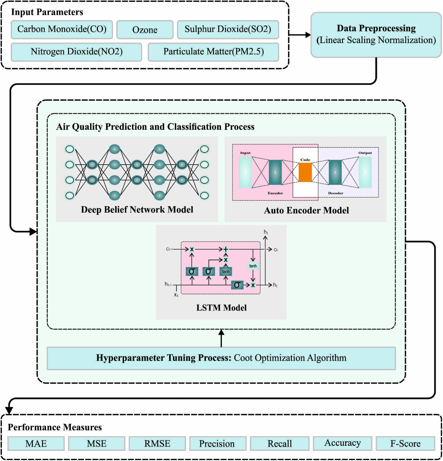
Figure 1: Overall flow of COAEDL-APP approach

3.1 Data Pre-Processing

Primarily, the feature dataset is pre-processed utilizing LSN. The problem of huge number ranges being dominated can be avoided by normalising the database features that support the algorithm in making correct forecasts [19]. Because of this, a pre-processing approach can be developed to turn the data into a maximal linear-scaling transformation. Normalized has been utilized for turning the observed data into values between zero and one across the investigation time. Afterwards, the scaled hourly data has been employed to represent the average daily energy procedure. LSN can be determined by Eq. (1).

yi′=yi−yminymax−ymin(1)

whereas max and min signify the maximal and minimal values of features correspondingly. ymin refers to the input database’s actual value as yYi, the normalizing value scaled based on the range.

3.2 Air Pollution Prediction Using Ensemble Learning

For air quality prediction, an ensemble of three DL models was involved, namely AE, LSTM, and DBN. AEs are unsupervised learning approaches which can be employed for learning the compact representation of the input data and collecting the highly related features of air pollution. At the same time, the LSTM models can be proficiently used to learn patterns in the time series data. By training an LSTM model on historical air pollution data, it can be employed for forecasting future pollution levels based on past observations. In the context of air pollution, a DBN can be trained on various features such as meteorological data, traffic information, and historical pollution levels. Once trained, the model can be used to predict air pollution levels based on the input features.

Let us have a trained set and a group of classifiers as h1, h2, … , hn, and every classifier has been trained on the trained set. Therefore, after training, the classifier produces forecasts. The classifier h1 makes the prediction y1; classifier h2, prediction y2; and classifier hn, prediction yn. For each novel data point, it takes n predictions. Next, it can take voting to arrive at the last forecast. The voting decreases n classes forecasts to a single data point as a single class. Thus, it can be utilized in majority voting to decide the last vote. The mode function can be utilized for obtaining the last vote that is written in Eq. (2).

yf=mode{h1(x), h2(x),…, hn(x)}(2)

where hi(x)=yi(x).

3.2.1 AE Model

AE are extensively applied in the model generation, data dimension reduction, and effective coding and is mostly used for automatically learning non-linear data feature [20]. When the amount of neurons in the output and input layers is m, the amount of neurons in the hidden layer (HL) is n, and the HL data has been signified as H={h1,h2,…,hn} and the input data can be signified as X={x1,x2,…, xm}. The output layer is X′={x1′,x2′,…,xm}.

The basic framework of AE is divided into encoding and decoding. The network that converts the higher dimension data X of the input layer to lower dimension HL is named encoding. The function f is deterministic mapping. This procedure is formulated as follows:

H=f(x)=sf(WX+b)(3)

In Eq. (3), the decoder converts the HL data H via function g to attain the reconstruction output layer dataset, X′. W shows the mapping weighted matrix of n×m dimensional. sf signifies the activation function of encoded. b∈Rn denotes the bias vector. This can be formulated as follows:

X′=g(H)=sg(W′H+b′)(4)

In Eq. (4), W′ signify the mapping weight matrix size of m×n. sf and sg Encoder and decoder activation functions implement well in learning features through the non-linear activation function. Tb′∈Rm indicates the bias vector. AE constantly trains the input dataset X and X′ to minimalize the reconstructed error term such that X and X′ are as close as possible to accomplish better-reconstructed outcomes. In general, the cross entropy computation is applied for reconstructing the error term:

E(X,X′)=−∑i=1n(xilog xi´′+(1−xi) log (1−xi′))(5)

The AE defines the mapping among the lower and higher dimension data without the loss of the data. Thus, the amount of neurons from the HL of the AE is lesser than the number of neurons from the input layer m.

3.2.2 LSTM Model

LSTM is a special variety of RNNs and is appropriate to process and predict significant events with comparatively long delays and intervals from the time sequence data [21]. Because of the capability of LSTM for learning long-term dependency, it resolves the issue of gradient explosions and disappearance in classical NN.

The basic framework of the LSTM involves update, forget, input, and output gates. A set of data can be inputted to the LSTM model. Only the data that meets the algorithm validation can be stored by the memory unit, and the data which dose not match can be forgotten by forgot gate. The specific Eqs. (6) to (11) of LSTM are given below:

ft=σ(Wf(ht−1′xt)+bf)(6)

it=σ(Wi(ht−1′xt)+bi)(7)

gt=tanh(Wg(ht−1′xt)+bg)(8)

ct=ftct−1+itgt(9)

0t=σ(W0(ht−1′xt)+b0)(10)

ht=0ttanh (c)(11)

From the expression, ct signifies the storage unit used for storing relevant data; ft, it, gt, and 0t correspondingly represent the output value of forget, input, update, and output gates; Wf, Wi, Wg, and W0 indicates the weight vector; bf, bi, bg, and b0 show the deviation vector; σ indicates the sigmoid function and maps real numbers within the range (0,1).

3.2.3 DBN Model

DBN contains a multilayer probabilistic ML method. Conventional MLP faces gradient dis-appearance problems, the fact of taking more hours, and the immense necessity for training data; however, it was a practical DL technique to manage such disadvantages [22]. It has supervised and unsupervised learning processes, where a network accomplishes an unsupervised learning framework with many layers of RBM bodies, and supervised learning is executed by the BP networks layer. Unsupervised learning completed the initialization of the variable of all layers of the network, while supervised learning fine-tuned the initialized parameters.

An RBM has HL and a visible layer (VL). The HL and VL were linked in both directions; however, the nodes of all layers are not linked with one another. At the time of the RBM learning process, an energy function E(v,h|θ) must be described, and a usually utilized resolves formula of the energy function is given below:

E(v,h|θ)=−∑i=1n∑j=1mωijvihj−∑i=1nbivi−∑j=1mcjhj(12)

Here v=(v1,v2, …,vn)T indicates the VL, h=(h1,h2, …,hm) means the HL, ω=(ωi,j)∈Rn×m denoted the weight matrix linking two layers and b=(b1,b2, …,bn)T, c=(c1,c2, …,cm)T denoted the bias of v, h correspondingly θ={ωij,bi,cj} signify an RBM parameter set.

This RBM framework allowed the values of the HL and VL to be uncorrelated from one another. As a replacement for computing all neurons simultaneously, the complete layer is calculated simultaneously. Afterwards, the probability distribution of the hidden and VLs is:

p(v,h|θ)=e−E(v,h|θ)/Z( )(13)

Z(θ)=∑v⁡∑h⁡e−E(v,h|θ)(14)

p(hj=1|v, θ)=f(cj+∑i=1nωijvi)(15)

As the RBM layers are linked in both directions, neurons presented in VL, vi can be stimulated by neurons hj in HL, and its probability is given below:

p(vi=1|h, θ)=f(bi+∑j=1mωijhj)(16)

The RBM training procedure learned the value of the variable θ to fit the given training dataset. The non-supervised learning procedure generally utilizes the CD technique to upgrade the variables, and the upgrade rules for all variables are given below:

Δω=ε(Edata(vihj)−Erecon(vihj))(17)

Δc=ε(Edata(hj)−Erecon(hj))(18)

Δb=ε(Edata(vi)−Erecon(vi))(19)

Here ε denoted the learning rate for RBM training, Eecon signify the expectation over distribution described by the reconstructed model, and Edata denoted the mathematical expectation over distribution described by the training dataset. A layer of supervised BPs and various unsupervised RBMs form complete DBN.

3.3 Hyperparameter Tuning Using COA

Finally, the COA can be used to adjust the hyperparameter values of the DL models. COA is a new optimization technique stimulated by the behaviours of coot birds [23]. Some coots floating on the water’s surface can be responsible for the flock’s guidance. Moving in chains, random wandering, shifting the position concerning the group leader, and guiding the pack to the optimum place are the four approaches of COA. This behaviour could not be performed without the mathematical expression. Fig. 2 depicts the flowchart of COA.

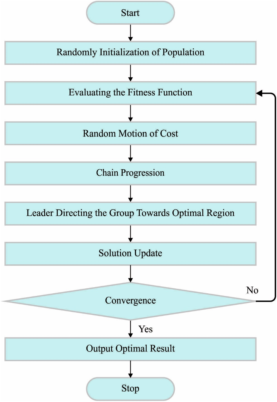
Figure 2: Flowchart of COA

The initial condition includes the generation of a random population of coots.

PosCoot(i)=random (1,D)×(UB−LB)+LB,i=1,2,…,N(20)

Eq. (20) produces the uniform distribution of coot position in a high dimensional space based on the upper limits UB and lower boundaries LB evaluated for every dimension. The coot could not go below or beyond the protection level.

F(i)=Fitness (PosCoot(i)),i=1,2,…,N(21)

Firstly, an arbitrary place can be produced by applying Eq. (22) to characterize the unpredictable behaviour of coots. Next, the new location of the coot can be calculated as follows:

R=random(1,D)×(UB−LB)+LB(22)

PosCoot (i)=PosCoot(i)+A×RN2×(R−PosCoot(i))(23)

A=1−(T(i)×1IterMax), B=2−(T(i)×1IterMax) i=1,2,…, IterMaχ(24)

PosCoot(i)=0.5×(PosCoot(i−1)+PosCoot(i))(25)

Also, Coot selects a leader coot and shadows them based on Eq. (26):

Lind=1+(iMODNL)(26)

where NL denotes the parameterized amount of leaders, and Lind indicates the leader index.

LeaderPos(i)={B×R3×cos⁡(2Rπ)×(gBest−LeaderPos(i)+gBestR4<P)B×R3×cos⁡(2Rπ)×(gBest−LeaderPos(i)+gBestR4≥P)}(27)

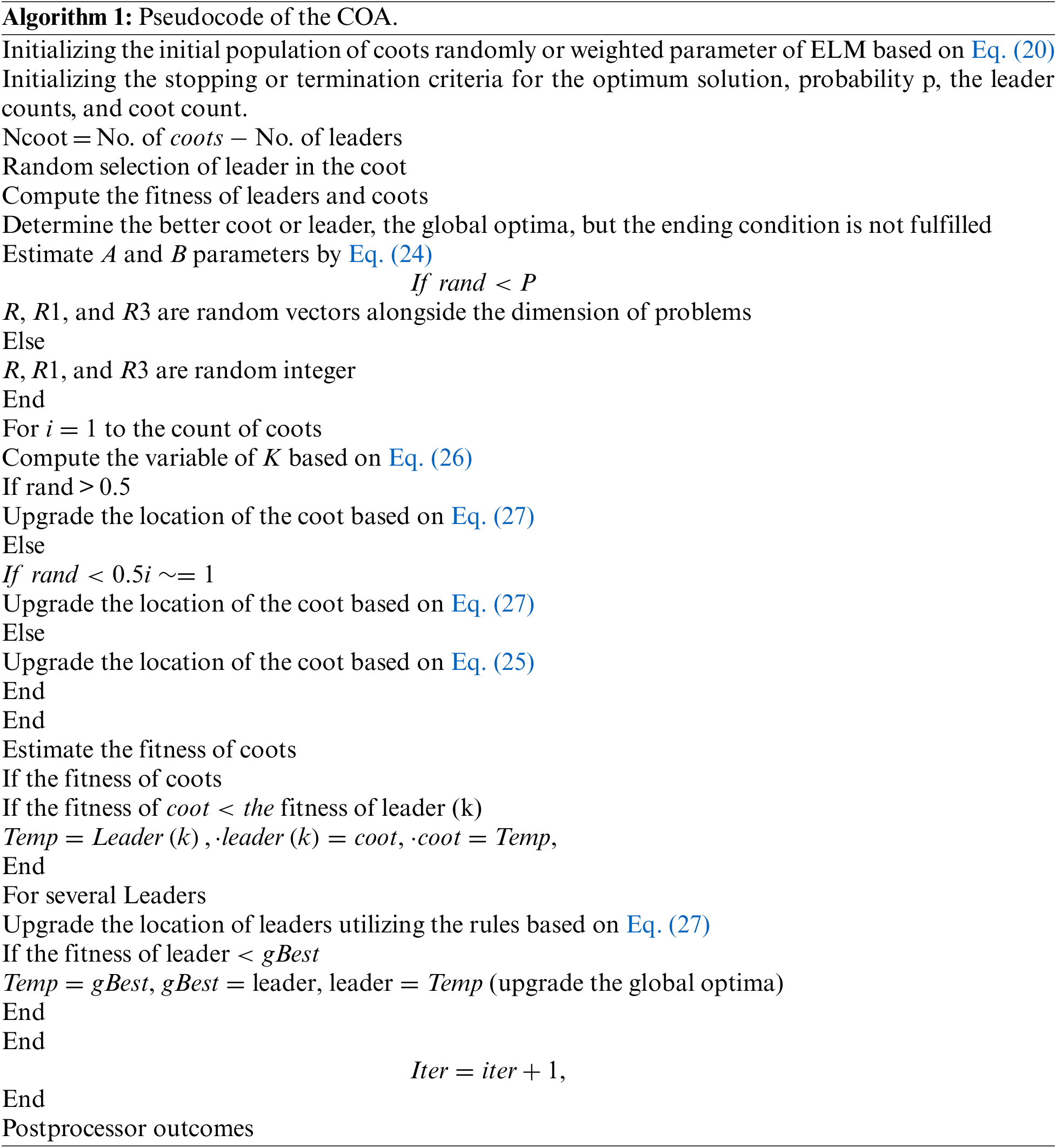
The pseudocode of COA is given in Algorithm 1.

During this case, the COA can be utilized for determining the hyperparameter contained in the DL technique. The MSE can be regarded that the main function and is determined as:

MSE=1T∑j=1L∑i=1M(yji−dji)2(28)

In which M and L signify the outcome value of layer and data correspondingly, yji and dji represent the achieved and suitable magnitudes for the jth unit in the outcome layer of the network in time t correspondingly.

4  Results and Discussion

The proposed model is simulated using Python 3.6.5 tool. The proposed model is experimented on PC i5-8600k, GeForce 1050Ti 4 GB, 16 GB RAM, 250 GB SSD, and 1 TB HDD. The parameter settings are given as follows: learning rate: 0.01, dropout: 0.5, batch size: 5, epoch count: 50, and activation: ReLU.

The COAEDL-APP approach is validated utilizing a dataset including various air quality parameters, namely Ozone, Nitrogen dioxide (NO2), Particulate Matter (PM2.5), Sulphur dioxide (SO2), and Carbon monoxide (CO). The database holds an entire of 22321 instances. The AQI values can be grouped into 6 distinct classes. Besides, the good and moderate values come under the ‘Non-Pollutant’ class (15738 instances), and the residual values come under the ‘Pollutant’ class (6583 instances).

In Table 1, the overall predictive result of the COAEDL-APP technique is demonstrated. Fig. 3 highlights the MAE results of the COAEDL-APP system under distinct variables. The outcomes indicate that the COAEDL-APP methodology reaches reduced MAE values under all values. For instance, with CO, the COAEDL-APP technique attains MAE of 0.108 and 0.287 under TRS and VLS. Along with that, with NO2, the COAEDL-APP approach reaches MAE of 0.093 and 0.205 under TRS and VLS. Meanwhile, with PM2.5, the COAEDL-APP algorithm gains MAE of 0.124 and 0.345 under TRS and VLS.

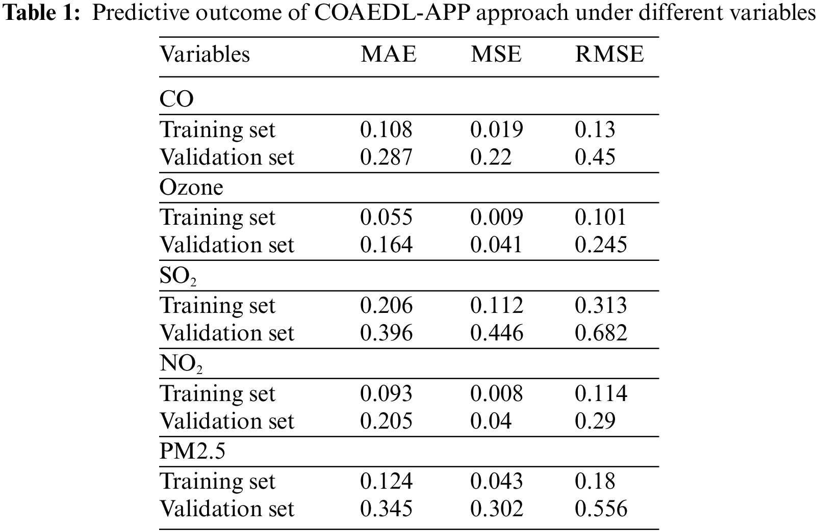
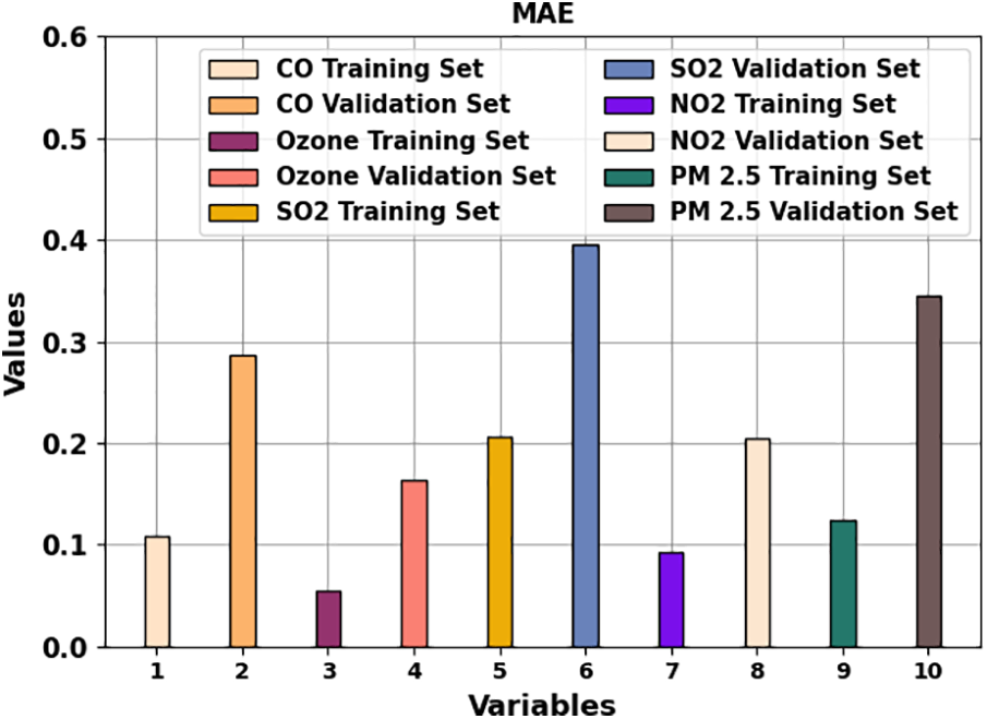
Figure 3: MAE analysis of the COAEDL-APP approach

Fig. 4 illustrates the MSE outcomes of the COAEDL-APP approach under distinct variables. The outcomes implied that the COAEDL-APP system reaches reduced MSE values under all values. For instance, with CO, the COAEDL-APP algorithm reaches MSE of 0.019 and 0.22 under TRS and VLS. Along with that, with NO2, the COAEDL-APP system reaches MSE of 0.008 and 0.04 under TRS and VLS. In the meantime, with PM2.5, the COAEDL-APP algorithm gains MSE of 0.043 and 0.302 under TRS and VLS.

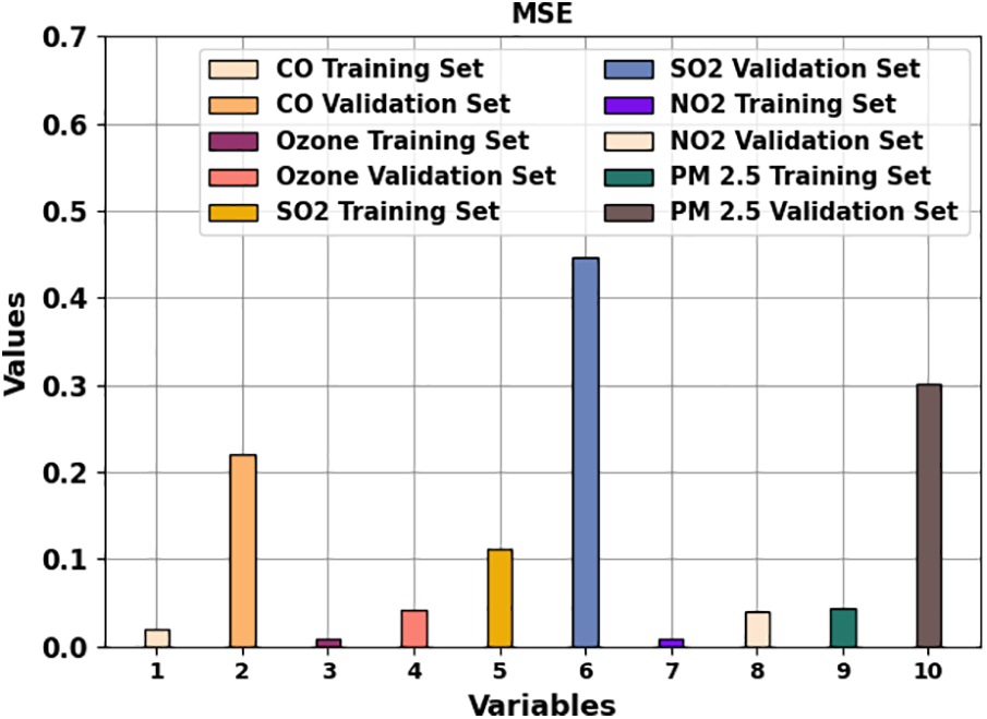
Figure 4: MSE outcome of COAEDL-APP algorithm

Fig. 5 demonstrates the RMSE results of the COAEDL-APP method under different variables. The results indicate that the COAEDL-APP method obtains lower RMSE values under all values. For instance, with CO, the COAEDL-APP technique attains RMSE of 0.13 and 0.45 under TRS and VLS. Along with that, with NO2, the COAEDL-APP methodology attains RMSE of 0.114 and 0.29 under TRS and VLS. Eventually, with PM2.5, the COAEDL-APP algorithm gains RMSE of 0.18 and 0.556 under TRS and VLS.

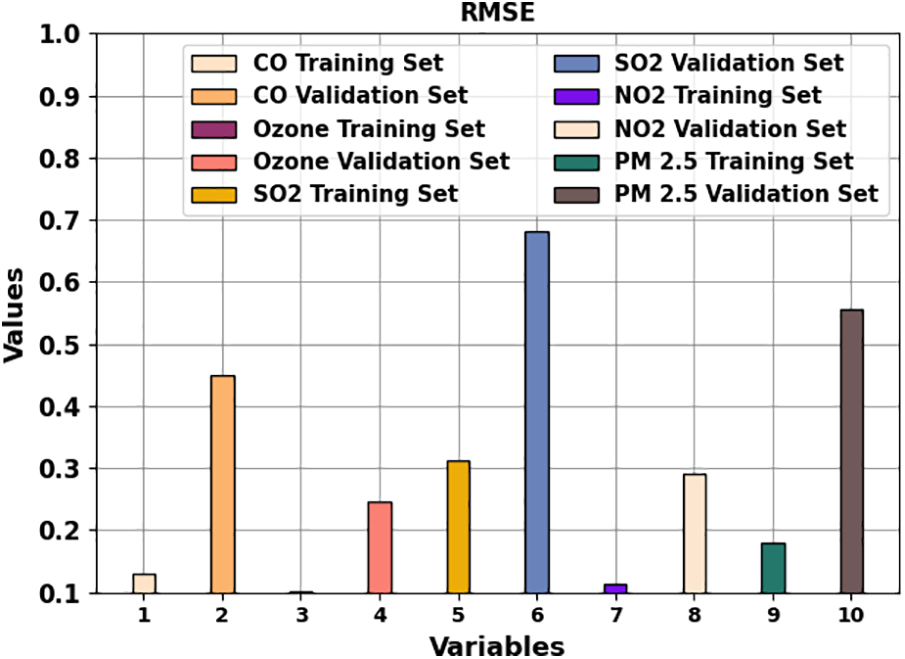
Figure 5: RMSE outcome of COAEDL-APP algorithm

The confusion matrices of the COAEDL-APP algorithm on air pollution classification are demonstrated in Fig. 6. The outcomes highlighted that the COAEDL-APP system has correctly identified the pollutants and non-pollutants under all folds.

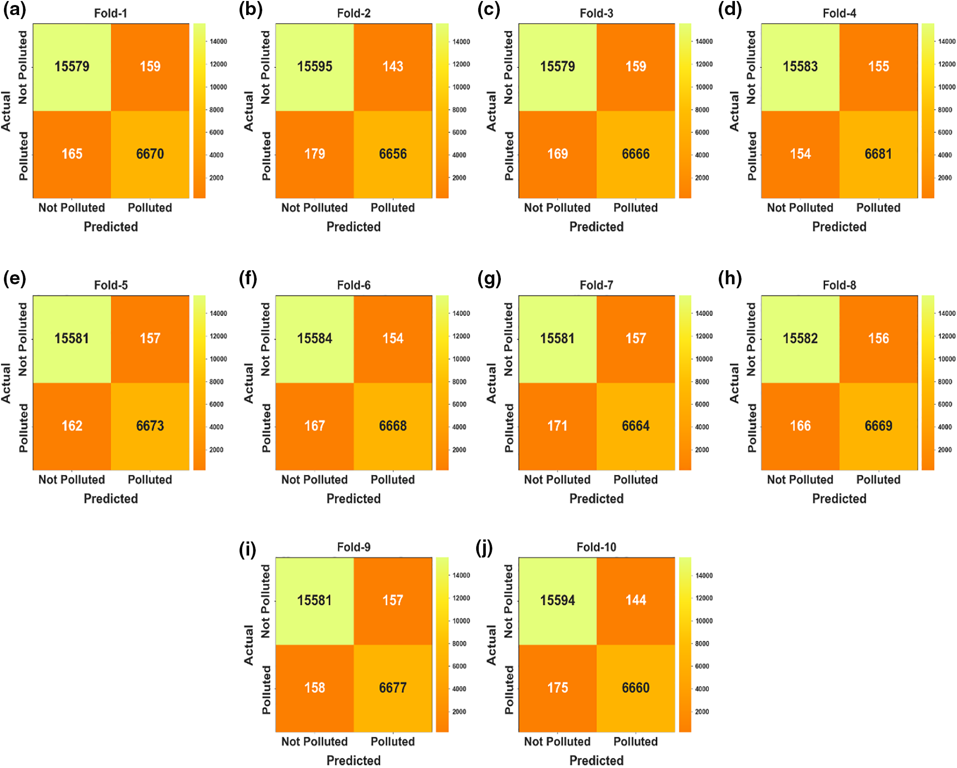
Figure 6: Confusion matrices of COAEDL-APP approach (a–j) Fold 1–10

In Table 2 and Fig. 7, an overall air pollution classification result of the COAEDL-APP technique is elaborated. The results indicate that the COAEDL-APP technique reaches improved classification results under all folds. For sample, on fold-1, the COAEDL-APP algorithm obtains accuy of 98.29%, precn of 98.31%, recal of 98.29%, and Fscore of 98.30%. Meanwhile, on fold-3, the COAEDL-APP approach gains accuy of 98.26%, precn of 98.30%, recal of 98.26%, and Fscore of 98.28%. Eventually, on fold-7, the COAEDL-APP algorithm reaches accuy of 98.25%, precn of 98.31%, recal of 98.25%, and Fscore of 98.28%. At last, on fold-10, the COAEDL-APP system attains accuy of 98.26%, precn of 98.39%, recal of 98.26%, and Fscore of 98.32%.

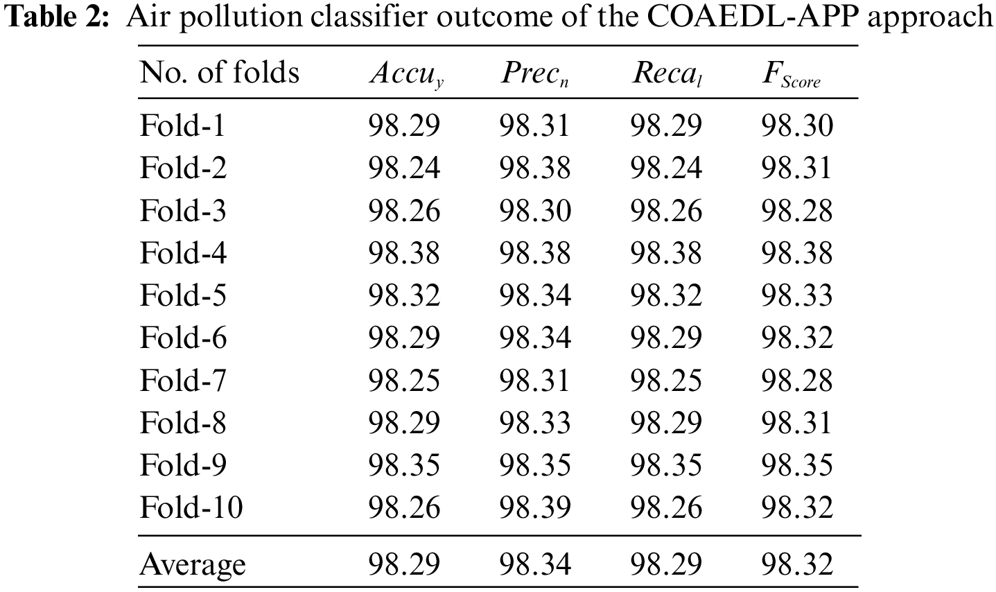
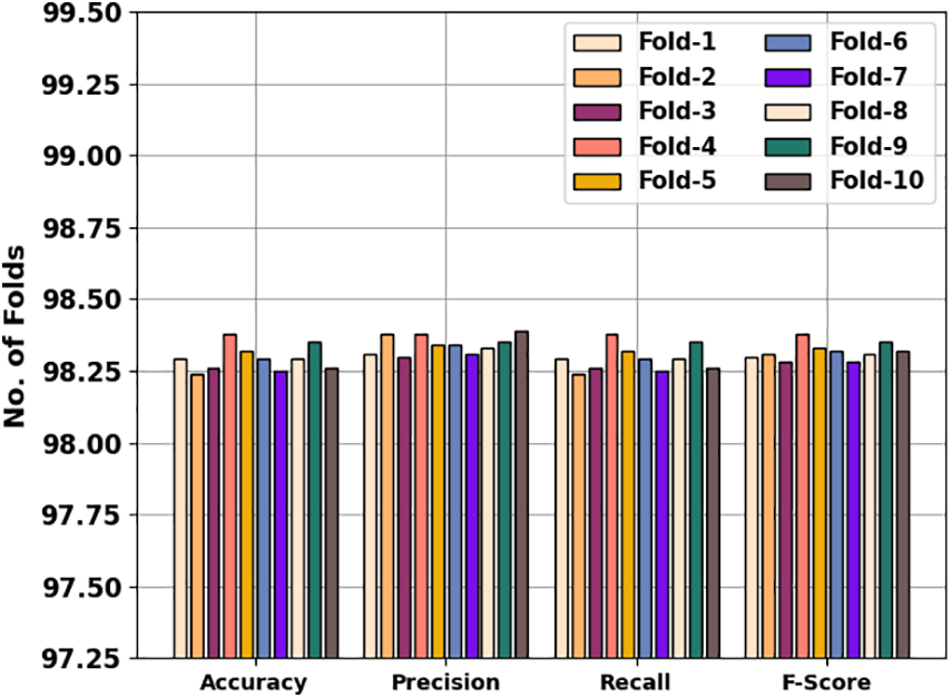
Figure 7: Air pollution classifier outcome of COAEDL-APP approach

In Fig. 8, an average air pollution classification result of the COAEDL-APP technique is stated. The results indicate that the COAEDL-APP technique reaches effectual outcomes with an average accuy of 98.29%, precn of 98.34%, recal of 98.29%, and Fscore of 98.32%.

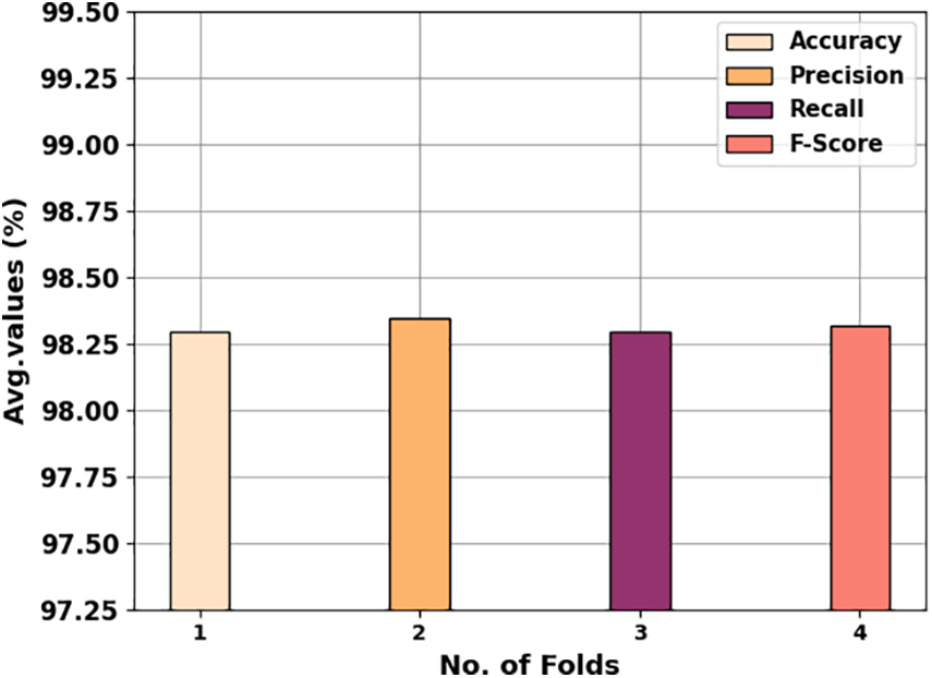
Figure 8: Average outcome of the COAEDL-APP approach

Fig. 9 inspects the accuracy of the COAEDL-APP algorithm during the training and validation process on the test dataset. The figure implies that the COAEDL-APP system gains increasing accuracy values over maximal epochs. Furthermore, the higher validation accuracy over training accuracy displays that the COAEDL-APP methodology learns efficiently on the test dataset.

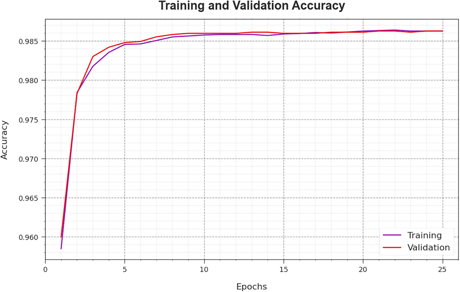
Figure 9: Accuracy curve of the COAEDL-APP approach

The loss investigation of the COAEDL-APP algorithm at the time of training and validation is represented on the test dataset in Fig. 10. The outcome implies that the COAEDL-APP approach attains closer values of training and validation loss. It is noted that the COAEDL-APP algorithm learns efficiently on the test dataset.

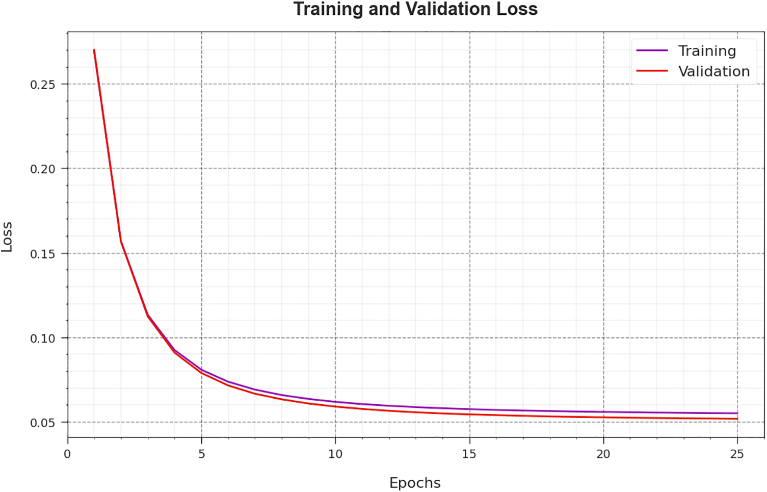
Figure 10: Loss curve of the COAEDL-APP approach

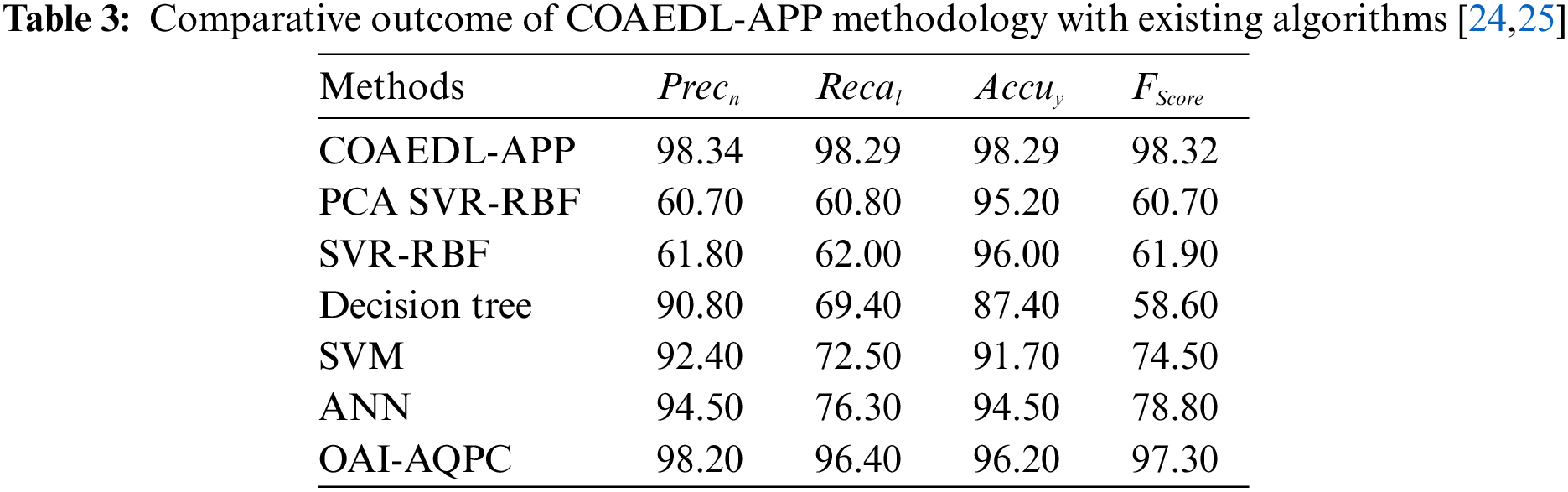
In Table 3 and Fig. 10, a clear comparison study of the COAEDL-APP method with existing models is made [24,25]. The outcomes indicate that the PCA SVR-RBF and SVR-RBF models obtain lower classification results. Followed by, the DT, SVM, and ANN models have managed to attain moderately closer classifier results. Along with that, the OAI-AQPC technique resulted in reasonable performance with precn of 98.20%, recal of 96.40%, accuy of 96.20%, and Fscore of 97.30%. However, the COAEDL-APP technique gains higher performance with precn of 98.34%, recal of 98.29%, accuy of 98.29%, and Fscore of 98.32%. These outcomes make sure the improved performance of the COAEDL-APP approach compared to methods.

5  Conclusion

In this article, we have presented a novel COAEDL-APP system to forecast air pollution levels in sustainable smart cities. The presented COAEDL-APP technique accurately forecasts the presence of air quality in the sustainable smart city environment. To achieve this, the COAEDL-APP technique follows a three-stage process, namely LSN-based pre-processing, ensemble DL-based prediction, and COA-based hyperparameter tuning. For air quality prediction, an ensemble of three DL models was involved, namely AE, LSTM, and DBN. Furthermore, the COA-based hyperparameter tuning process can be designed to adjust the hyperparameter values of the DL models. The simulation outcome of the COAEDL-APP algorithm was tested on the air quality dataset, and the outcomes stated the enhanced efficacy of the COAEDL-APP algorithm on other existing techniques. In future, the outcome of the COAEDL-APP technique was extended to the inclusion of IoT and big data environment in industrial sectors.

Acknowledgement: The authors gratefully acknowledge the technical and financial support provided by the Ministry of Education and Deanship of Scientific Research (DSR), King Abdulaziz University (KAU), Jeddah, Saudi Arabia.

Funding Statement: This research work was funded by the Deanship of Scientific Research (DSR), King Abdulaziz University (KAU), Jeddah, Saudi Arabia under Grant No. (IFPIP: 631-612-1443).

Author Contributions: Conceptualization and Methodology: Maha Farouk Sabir and Mahmoud Ragab; software and data curation: Adil O. Khadidos and Khaled H. Alyoubi; formal analysis: Mahmoud Ragab and Alaa O. Khadidos; writing—original draft, Maha Farouk Sabir, Mahmoud Ragab and Adil O. Khadidos; writing—review & editing: Khaled H. Alyoubi and Alaa O. Khadidos; project administration: Mahmoud Ragab; funding acquisition: Maha Farouk Sabir. All authors have read and agreed to the published version of the manuscript.

Availability of Data and Materials: Data sharing not applicable to this article as no datasets were generated during the current study.

Conflicts of Interest: The authors declare that they have no conflicts of interest to report regarding the present study.

References

1. S. Myeong and K. Shahzad, “Integrating data-based strategies and advanced technologies with efficient air pollution management in smart cities,” Sustainability, vol. 13, no. 13, pp. 7168, 2021. [Google Scholar]

2. M. Ragab and M. F. S. Sabir, “Outlier detection with optimal hybrid deep learning enabled intrusion detection system for ubiquitous and smart environment,” Sustainable Energy Technologies and Assessments, vol. 52, pp. 102311, 2023. [Google Scholar]

3. C. Magazzino, M. Mele and S. A. Sarkodie, “The nexus between COVID-19 deaths, air pollution and economic growth in New York state: Evidence from deep machine learning,” Journal of Environmental Management, vol. 286, pp. 112241, 2021 [Google Scholar] [PubMed]

4. A. I. Middya and S. Roy, “Pollutant specific optimal deep learning and statistical model building for air quality forecasting,” Environmental Pollution, vol. 301, pp. 118972, 2022 [Google Scholar] [PubMed]

5. M. Arsov, E. Zdravevski, P. Lameski, R. Corizzo, N. Koteli et al., “Multi-horizon air pollution forecasting with deep neural networks,” Sensors, vol. 21, no. 4, pp. 1235, 2021 [Google Scholar] [PubMed]

6. X. B. Jin, Z. Y. Wang, W. T. Gong, J. L. Kong, Y. T. Bai et al., “Variational Bayesian network with information interpretability filtering for air quality forecasting,” Mathematics, vol. 11, no. 4, pp. 837, 2023. [Google Scholar]

7. C. Magazzino, M. Mele and N. Schneider, “The relationship between air pollution and COVID-19-related deaths: An application to three French cities,” Applied Energy, vol. 279, pp. 115835, 2020 [Google Scholar] [PubMed]

8. M. Alghieth, R. Alawaji, S. H. Saleh and S. Alharbi, “Air pollution forecasting using deep learning,” International Journal of Online & Biomedical Engineering, vol. 17, no. 14, pp. 50–64, 2021. [Google Scholar]

9. M. Ragab, “Spider monkey optimization with statistical analysis for robust rainfall prediction,” Computers, Materials & Continua, vol. 72, no. 2, pp. 4143–4155, 2022. [Google Scholar]

10. C. Aarthi, V. J. Ramya, P. F. Gilski and P. B. Divakarachari, “Balanced spider monkey optimization with bi-lstm for sustainable air quality prediction,” Sustainability, vol. 15, no. 2, pp. 1637, 2023. [Google Scholar]

11. S. Li, G. Xie, J. Ren, L. Guo, Y. Yang et al., “Urban PM2.5 concentration prediction via attention-based cnn–lstm,” Applied Sciences, vol. 10, no. 6, pp. 1953, 2020. [Google Scholar]

12. P. Asha, L. Natrayan, B. T. Geetha, J. R. Beulah, R. Sumathy et al., “IoT enabled environmental toxicology for air pollution monitoring using AI techniques,” Environmental Research, vol. 205, pp. 112574, 2022 [Google Scholar] [PubMed]

13. B. Zhang, H. Zhang, G. Zhao and J. Lian, “Constructing a PM2.5 concentration prediction model by combining auto-encoder with Bi-LSTM neural networks,” Environmental Modelling & Software, vol. 124, pp. 104600, 2020. [Google Scholar]

14. J. Ma, Y. Ding, V. J. L. Gan, C. Lin and Z. Wan, “Spatiotemporal prediction of PM2.5 concentrations at different time granularities using IDW-BLSTM,” IEEE Access, vol. 7, pp. 107897–107907, 2019. [Google Scholar]

15. W. Du, L. Chen, H. Wang, Z. Shan, Z. Zhou et al., “Deciphering urban traffic impacts on air quality by deep learning and emission inventory,” Journal of Environmental Sciences, vol. 124, pp. 745–757, 2023. [Google Scholar]

16. T. Li, M. Hua and X. Wu, “A hybrid CNN-LSTM model for forecasting particulate matter (PM2.5),” IEEE Access, vol. 8, pp. 26933–26940, 2020. [Google Scholar]

17. H. W. Wang, X. B. Li, D. Wang, J. Zhao, H. He et al., “Regional prediction of ground-level ozone using a hybrid sequence-to-sequence deep learning approach,” Journal of Cleaner Production, vol. 253, pp. 119841, 2020. [Google Scholar]

18. M. A. A. Al-Qaness, H. Fan, A. A. Ewees, D. Yousri and M. Abd Elaziz, “Improved ANFIS model for forecasting Wuhan City air quality and analysis COVID-19 lockdown impacts on air quality,” Environmental Research, vol. 194, pp. 110607, 2021 [Google Scholar] [PubMed]

19. S. Sorguli and H. Rjoub, “A novel energy accounting model using fuzzy restricted boltzmann machine—Recurrent neural network,” Energies, vol. 16, no. 6, pp. 2844, 2023. [Google Scholar]

20. H. Zhu, Y. Shang, Q. Wan, F. Cheng, H. Hu et al., “A model transfer method among spectrometers based on improved deep autoencoder for concentration determination of heavy metal ions by UV-Vis spectra,” Sensors, vol. 23, no. 6, pp. 3076, 2023 [Google Scholar] [PubMed]

21. X. Chen and Z. Long, “E-commerce enterprises financial risk prediction based on fa-pso-lstm neural network deep learning model,” Sustainability, vol. 15, no. 7, pp. 5882, 2023. [Google Scholar]

22. G. P. Mohammed, N. Alasmari, H. Alsolai, S. S. Alotaibi, N. Alotaibi et al., “Autonomous short-term traffic flow prediction using pelican optimization with hybrid deep belief network in smart cities,” Applied Sciences, vol. 12, no. 21, pp. 10828, 2022. [Google Scholar]

23. K. Sridhar, C. Kavitha, W. C. Lai and B. P. Kavin, “Detection of liver tumour using deep learning based segmentation with coot extreme learning model,” Biomedicines, vol. 11, no. 3, pp. 800, 2023 [Google Scholar] [PubMed]

24. M. A. Hamza, H. Shaiba, R. Marzouk, A. Alhindi, M. M. Asiri et al., “Big data analytics with artificial intelligence enabled environmental air pollution monitoring framework,” Computers, Materials & Continua, vol. 73, no. 2, pp. 3235–3250, 2022. [Google Scholar]

25. M. Castelli, F. M. Clemente, A. Popovic, S. Silva and L. Vanneschi, “A machine learning approach to predict air quality in California,” Complexity, vol. 2020, no. 332, pp. 1–23, 2020. [Google Scholar]