A New Malicious Code Classification Method for the Security of Financial Software

1  Introduction

The importance of financial software security is self-evident. With the rapid development of financial technology, financial software has penetrated into all aspects of our daily lives, from online payments to e-banking, from investment and wealth management to insurance business, almost everywhere. Therefore, ensuring the security of financial software not only relates to the reputation and interests of financial institutions, but also directly affects the property security and personal privacy of the majority of users.

Financial software is a platform for processing highly sensitive data, including users’ identity information, bank accounts, transaction records, credit card information, etc. Once this data is leaked or illegally used, it will cause huge economic losses and a crisis of trust to individual users and businesses. Therefore, ensuring the safe and stable operation of financial software and preventing data leaks and unauthorized access is the primary task of the financial industry.

In addition, the security of financial software is also directly related to the stability of the financial market and the economic security of the country. In the context of globalization, the financial market is increasingly becoming a complex network system, and the links between the financial markets of various countries are getting closer. Once a security vulnerability appears in an important financial software, it may trigger a chain reaction, causing impact on the entire financial market, and even affecting the economic security of the country.

Therefore, we must attach great importance to the security issues of financial software, and continuously improve the security protection capabilities of financial software through various measures such as strengthening technology research and development, improving the regulatory system, and improving the quality of practitioners. Only in this way can we ensure that while promoting economic and social development, financial technology will not become a hidden danger and source of risk.

The presence of malicious code in financial software poses serious hazards. Since financial software involves extensive fund flows and the processing of sensitive information, the successful infiltration of malicious code can lead to significant economic losses and privacy breaches.

Firstly, malicious code can steal users’ personal and financial data. By intercepting sensitive information such as account passwords, credit card details, or transaction records, the creators of malicious code can gain illegal access to users’ assets and engage in various fraudulent activities. This not only results in financial losses for individual users but can also severely impact the reputation and operations of financial institutions.

Secondly, malicious code can tamper with financial transactions and operations. By modifying crucial information such as transaction amounts, beneficiaries, or trading instructions, malicious code can cause erroneous executions or illegal transfers of funds. Such tampering disrupts the fairness and transparency of financial markets, and may lead to disputes and legal risks.

In addition, malicious code can leverage financial software for malicious attacks and cybercrimes. For example, it can exploit vulnerabilities in financial software to launch denial-of-service attacks, rendering financial institutions’ systems inoperable. Alternatively, malicious code can serve as a tool for cybercrimes such as money laundering, illegal fund transfers, or other illegal activities.

Therefore, the hazards posed by malicious code in financial software are immense and require heightened attention. Financial institutions should strengthen security measures, including regular software updates, timely patching of vulnerabilities, implementation of strict access controls and security audits, to ensure the safety and trustworthiness of financial software. Meanwhile, users should also raise their security awareness, avoid downloading and installing untrusted software, regularly update operating systems and security software, and promptly report suspicious activities. Only through collective efforts can we effectively address the threats posed by malicious code in financial software.

Embedded malicious code within financial software can pose grave threats to both the financial system and individual clientele, underscoring the criticality of detecting such code prior to software installation. The proliferation of malicious code on the Internet has ballooned to become a substantial menace to cybersecurity. According to the China Cybersecurity Report 2020 [1], the cloud security system from Rising intercepted a staggering 148 million virus samples and 352 million virus infections in 2020, with an overall surge of 43.71% in viruses compared to 2019. Moreover, attackers often resort to various obfuscation techniques to modify malicious code, evading detection by antivirus software, thereby bolstering the malicious code’s concealment capabilities and compounding the challenges in virus detection. Effective identification of malicious code and its variants remains one of the most daunting challenges in cybersecurity today. Given the evolving nature and intricacy of malware, the capacity to combat it must also undergo continuous evolution, necessitating relentless efforts to enhance detection methodologies and stay ahead of the constantly morphing cyber threats.

Malicious code detection typically falls into two categories: Static and dynamic detection. Static detection involves the use of a disassembler to convert the malicious code into readable binary source code [2], followed by an extraction of features such as opcodes and APIs for analysis, without executing the code. In contrast, dynamic detection entails running the code in a secure [3], controlled virtual environment and monitoring the operating system’s resource scheduling behavior induced by the malicious code. However, these conventional methods often rely on extensive manual feature engineering, which can be time-consuming, and may struggle to effectively identify variants of malicious code.

Malicious code variants are commonly produced by reusing code from the original malicious code, resulting in shared traits among different families of malicious code that can be identified through the texture features of images. In recent times, researchers have leveraged this similarity by representing malicious code binary files as images, grounded in traditional detection techniques, and subsequently integrating them with deep learning for the classification of malicious code families.

Convolutional Neural Networks (CNN) are a shining beacon in the field of deep learning, particularly renowned for their prowess in computer vision tasks [4]. By introducing convolutional operations, CNNs achieve local connectivity and weight sharing in input data, effectively reducing model complexity and enhancing performance.

The basic structure of a CNN comprises an input layer, convolutional layers, activation layers, pooling layers, and fully connected layers.

Input Layer: The input layer receives the raw data, such as pixel values for images. In image processing, the input layer typically converts the image into a two-dimensional matrix where each element represents the grayscale value (for grayscale images) or RGB value (for color images).

Convolutional Layers: These are the heart of CNNs, extracting features through convolution operations on the input data. Convolution involves sliding a filter (or kernel) over the input data, multiplying each element of the filter with its corresponding element in the input, and summing them up to create a new feature map. Various parameters like kernel size, stride, and padding can be adjusted based on requirements. Multiple kernels in a convolutional layer capture different features from the input data, enabling automatic feature learning.

Activation Layers: Activation layers introduce non-linearity to the output of convolutional layers, enhancing the model’s expressive capabilities. Common activation functions include ReLU (Rectified Linear Unit), Sigmoid, and Tanh. ReLU is widely preferred due to its simplicity, efficiency, and ability to mitigate the vanishing gradient problem.

Pooling Layers: Pooling layers are responsible for downsampling the output from convolutional or activation layers, reducing the number of parameters and computations while improving the model’s generalization ability. Common pooling operations include max pooling, which divides the input into sub-regions and outputs the maximum value from each, and average pooling, which outputs the average value.

Fully Connected Layers: These lie at the end of a CNN, integrating features extracted by previous layers to output final classification or regression results. Each neuron in a fully connected layer is connected to all neurons in the previous layer, justifying its name. In practice, multiple fully connected layers are often stacked to build deeper networks and improve model performance.

The strengths of CNN are multifaceted:

Local Connectivity: Unlike traditional neural networks, neurons in a CNN are connected only to a local region of the input data, reducing the number of parameters and simplifying the model. This approach aligns with the local receptive field characteristic of the human visual system.

Weight Sharing: In CNNs, the same filter is applied to different locations of the input data, achieving weight sharing. This further reduces the number of parameters and enables the model to learn spatial structure information from the data.

Hierarchical Feature Extraction: CNNs extract features from input data hierarchically through multiple convolutional layers, progressing from simple low-level features (such as edges and corners) to complex high-level features (like object shapes and textures). This hierarchical approach allows CNNs to automatically learn inherent structures and patterns in data.

Leveraging these strengths, CNNs have achieved remarkable successes in computer vision tasks such as image classification, object detection, and image segmentation. With the continuous advancement of deep learning technology, CNNs are also finding applications in areas like natural language processing and speech recognition, demonstrating their cross-domain versatility.

These networks possess the remarkable capability to autonomously learn features from input data, eliminating the need for manual intervention. Cui et al. [5] introduced a CNN-based detection model for malware variants. This model converts malicious code into grayscale images and employs the BAT algorithm to mitigate the class imbalance issue commonly observed within numerous malicious code sample families. Wang et al. [6] presented a detection model for malicious code families that combines CNN with Bidirectional Long Short-Term Memory (BiLSTM). This model possesses the ability to autonomously learn features from grayscale images of malicious code, thus substantially reducing the costs associated with manual feature extraction. Moreover, BiLSTM is endowed with the capacity to focus on both local and global features within the input data, thereby facilitating a more comprehensive understanding of contextual information.

To reduce computational demands, this study chose the static analysis method over the dynamic analysis method due to its significantly lower time and resource requirements. This approach involves reverse engineering techniques to extract features, which are then used for model construction. Extractable features include string features [7], opcode features [8], executable file structure features [9], and function call graph features [10]. Opcodes, which are machine-level instructions that describe program execution operations, are both practical and reliable. The n-gram method is used to extract opcodes due to its strong likelihood estimation capabilities and ease of understanding. After feature extraction, a model is constructed to classify malicious families. Previous studies have proposed methods for detecting the maliciousness of unknown programs by calculating opcode frequency values as features from the code or extracting opcode sequences from disassembled files to represent the temporal nature of malware execution [11,12]. Since Nataraj et al. initially introduced the conversion of malware executable files into two-dimensional grayscale maps, image texture features have become widely adopted in the domain of malware due to their similarity within each family for training.

Deep learning algorithms have undergone rapid advancements in areas like natural language processing, boasting powerful learning capabilities and offering advantages in mining data structures within high-dimensional data. These algorithms have found widespread application in the domain of malware detection, with Recurrent Neural Networks (RNNs) [13] and Gated Recurrent Units (GRUs) being commonly employed for malware detection. Kwon et al. [14] introduced a method that utilizes RNNs to classify malware based on API call functions. Through dynamic analysis, they extracted nine representative API call functions from various malware families to create a training dataset and subsequently employed Long Short-Term Memory (LSTM) for classification, achieving an average accuracy of 71%. Messay-Kebede et al. [15] proposed a detection model that combines traditional machine learning techniques with autoencoder-based methods. The traditional machine learning model handles the identification of some classes, while others are classified using autoencoders. Gibert et al. [16] extracted byte and opcode sequences and fed them into a classifier composed of two Convolutional Neural Networks (CNNs). Despite the relative simplicity of this structure, its accuracy was not superior to more complex classifiers. Yan et al. [17] presented Malnet, a detection model that employs CNNs to learn features from grayscale maps and LSTMs to learn opcodes. The classifications are then merged using a straightforward weighting approach. Narayanan et al. [18] adopted a CNN-LSTM approach for feature extraction and utilized two types of machine learning algorithms for classification: Support Vector Machines and Logistic Regression. Ahmadi et al. [19,20] extracted 15 and 6 features from malware, respectively, enabling more comprehensive information extraction. However, the processes of feature extraction and selection were time-consuming and encompassed features with minimal impact on classification.

As malicious code variants continue to grow in diversity, shallow Convolutional Neural Networks (CNNs) are becoming increasingly inadequate for capturing intricate texture features. This has led to the adoption of deep CNNs for the detection of malicious code families, which includes networks such as AlexNet [21], VGGNet [22], GoogleNet [23], and ResNet [24]. These network architectures progressively increase the depth and width of the network, facilitating the extraction of more intricate features. Jiang et al. [25] proposed an approach for detecting malicious code based on multi-channel image features and AlexNet. Multi-channel images provide a richer set of texture features compared to second-order grayscale images. Wang et al. [26] utilized VGGNet to develop a classification model for malicious samples, enabling the classification and detection of RGB images of malicious code while achieving improved recognition accuracy. Although deepening the network depth improves malicious code recognition efficiency to some extent, it also poses challenges such as model gradient explosion and a significant increase in the number of parameters, which requires considerable computational resources.

To overcome the limitations of current malicious code detection models in terms of recognition rates for malicious code and its variants, as well as their considerable number of parameters, this paper introduces a lightweight malicious code family detection model based on Ghost-DenseNet-SE. This approach utilizes the Dense Convolutional Network (DenseNet) as the backbone architecture, mitigating issues related to gradient disappearance and a substantial increase in parameters. The Ghost module replaces the convolutional layer within the Dense Block, generating supplementary feature mappings through a sequence of linear operations. This not only diminishes the count of model parameters but also guarantees detection precision, a lightweight framework, and adaptability to platforms with restricted resources. The channel domain attention mechanism enhances precise classification of malicious code families by assigning differing weights to feature channels. The squeeze-and-excitation (SE) channel attention mechanism further amplifies the number of model parameters. The Ghost module produces additional feature mappings via linear operations, reducing the model’s parameter count while preserving detection accuracy. By harnessing Ghost-DenseNet-SE, the proposed model effectively tackles the challenges of identifying malicious code and its variants while also minimizing the computational burden required for precise detection. This lightweight design allows for deployment on platforms with limited resources, bolstering the overall security posture.

2  Basic Theory

2.1 DenseNet

DenseNet, fully known as Densely Connected Convolutional Networks, is an innovative deep learning network architecture. This network structure was designed to address the issue of vanishing gradients that arise during the training of deep neural networks, improve the efficiency of feature propagation, and achieve efficient utilization of model parameters.

The core idea of DenseNet is dense connectivity, which introduces the concept of dense blocks in Convolutional Neural Networks (CNNs). Within a dense block, each layer is directly connected to all preceding layers, enabling the reuse of features and rapid information propagation. This connectivity not only helps to alleviate the vanishing gradient problem but also allows the network to learn richer and more complex feature representations.

The DenseNet architecture mainly consists of dense blocks, transition layers, and a global average pooling layer. Dense blocks are responsible for feature extraction and propagation, while transition layers control the size of feature maps and reduce computational costs. The global average pooling layer, located at the end of the network structure, converts the final feature maps into globally aggregated features suitable for tasks such as classification.

Compared to traditional convolutional neural networks, DenseNet offers the following advantages:

•   Effective mitigation of vanishing gradients: Through dense connectivity, each layer can directly access gradient information from all preceding layers, making the training process more stable.

•   More efficient feature propagation: Each layer can fully utilize feature information from all preceding layers, improving the efficiency of feature propagation.

•   Lesser computational requirements: Due to the reuse of features, DenseNet requires relatively less computation for comparable performance.

•   Fewer parameters: DenseNet reduces the number of parameters through parameter sharing, decreasing the complexity of the model.

Excellent performance: In practical applications, DenseNet has demonstrated superior performance compared to other advanced network architectures on various tasks and datasets.

The DenseNet, a CNN proposed by Huang et al. [27], features dense connectivity. This network structure is comprised of a Dense Block and a Transition layer, with the model structure depicted in Fig. 1. The DenseNet architecture includes several Dense Block modules, each constructed from BN-ReLU-Conv (3 × 3) components. The Transition layer situated between every two adjacent dense blocks consists of BN-ReLU-Conv (1 × 1) (with a filter number designated as “m”), dropout, and Pooling (2 × 2), where “BN” stands for Batch Normalization.

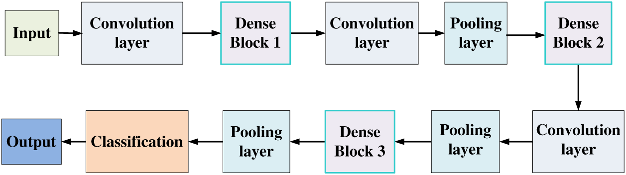
Figure 1: DenseNet structure

2.1.1 Dense Block

The Dense Block module exhibits a tight interconnection between any two of its layers. The internal structure, as depicted in Fig. 2, demonstrates that the features from all layers are concatenated; specifically, the output from all preceding layers is aggregated and serves as the input for any given layer. Subsequently, both the output of that layer and the output from the previous layer are relayed as the input for the succeeding layer. In contrast to a conventional CNN network which has L connections, a DenseNet with L layers would possess a total of L(L+1)/2 connections. This extensive interconnectivity is what qualifies it as a dense connection.

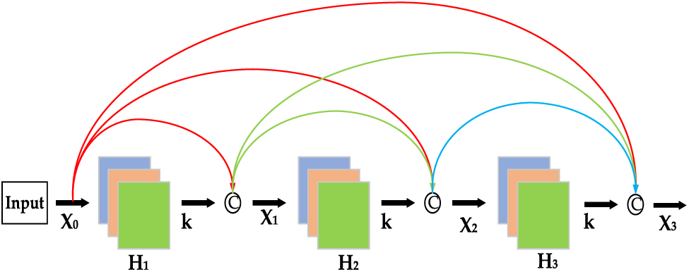
Figure 2: Dense block internal structure

For a network with L layers, the input of the l-th layer can be obtained through Eq. (1).

xl=H([x0,x1,…,xl−1])(1)

where x0,x1,…,xl−1 represents the feature maps corresponding from layer 0 to layer l−1; [x0,x1,…,xl−1] denotes the cascading of the corresponding feature maps from layer 0 to layer 1−1; and Hl(⋅) represents a composite function containing the operations of BN, Relu, and Conv.a

If each composite function Hl(⋅) in the Dense Block can output k feature maps, then layer l will input k0+k×(l−1) feature maps, where k0 represents the number of channels of the input layer channel. K, also known as the growth rate of the network, is a hyper-parameter that prevents the network from growing too fast. To decrease the number of network parameters so as to reduce the computational complexity, we add a bottleneck layer to the Dense Block; that is, a 1 × 1 convolution is introduced before the 3 × 3 convolution to reduce the dimensionality. The Dense Block structure after adding the bottleneck layer is BN+Relu+Conv(1 × 1)+BN+Relu+Conv(3 × 3), which is called the DenseNet-B model.

2.1.2 Transition Layer

The Transition layer is used to connect two adjacent Dense Blocks. It reduces the size of the feature map by pooling to make the model more compact. To further compress the model size, we introduce a compression factor θ, which uses the value range of (0,1]. When the Dense Block outputs m feature maps, the transition layer can produce features by convolution. When θ is less than 1, the number of feature maps is compressed to θ times that of the original; when θ is 1, no compression occurs. The structure of the transition layer after introducing the hyper-parameter θ is BN-Relu-Conv (1 × 1)(filternum: θ × m)-droupout-Pooling (2 × 2), which is called the DenseNet-C model.

When DenseNet uses both the Dense Block added to the bottleneck layer and the Transition layer with a compression factor (θ) less than 1, the network structure is called the DenseNet-BC model.

2.2 Channel Domain Attention Mechanism (SeNet)

The channel domain attention mechanism is often used in CNNs to visualize the important information of an image [28]. Each feature map is initially represented as three RGB channels. If the number of convolution kernels used for the feature channels is N, a matrix (H,W,N) of N new channels is generated after the convolution operation, with H and W denoting the height and width of the image features, respectively. The features of each channel represent the components of that feature map on different convolution kernels. The convolution of the convolution kernels is similar to the Fourier transform, which decomposes the information of this feature map channel into the signal components on N convolution kernels. Next, different weights are assigned to the signals of each channel. The larger the weight, the more critical the information in the feature map, and the more the network should pay attention to it. In contrast, the feature map is less important, and the network suppresses it. In this way, we extract important deep-level features in the image.

The core architectural unit of this mechanism is the SE Block [29], whose internal structure is shown in Fig. 3. First, the squeeze operation is applied to act on the feature map after the convolution pooling operation to obtain the global information of the feature map on the channel. Next, the excitation operation is used to obtain the laziness between the channels and obtain the weights of different channels, where the operation is the Sigmoid gate function. Finally, the final feature map is scaled.

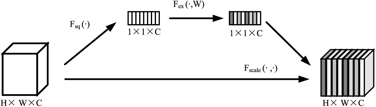
Figure 3: SE block internal structure

The squeeze operation is used to perform a global average pooling operation on the image, that is, to compress each feature map obtained in the spatial dimension. As a result, the global information of the c feature maps of the layer is obtained. The equation is given below:

Zc=Fsq(uc)=1W×H∑i=1W∑j=1Huc(i,j)(2)

The excitation operation is used to perform a fully connected layer operation on the 1 × 1 × C feature map obtained by squeeze, and it introduces a Reduction Ratio in the fully connected layer operation to reduce the number of channels and further reduce the amount of calculation. The results are then passed through the Sigmoid gate function to obtain the weights of C feature maps, where the weights represent the degree of dependency between channels. Finally, the neural network can learn the key information of different channels autonomously. The key information is expressed by s, with the equation

s=Fex(z,W)=σ(g(z,W))=σ(W2δ(W1z))(3)

where δ is the ReLU activation function, σ is the Sigmoid activation function, W1∈RC×Cr, W2∈RC×Cr, and r is the Reduction Ratio.

The aim of the scaling operation is to multiply the original feature channel value by different weights obtained through excitation, thereby enhancing the focus on the key channel domain of the original feature map to produce a new feature map and feed it to the next layer. The equation for this process is provided below:

XC=Fscale(uc,sc)=sc⋅uc(4)

2.3 Ghost Module

The Ghost module is a lightweight convolution module proposed by Han et al. from the redundancy problem of feature maps [30]. The module can be plug-and-play in the CNN networks to replace the traditional convolutional layer of the CNN. The traditional convolutional layer generates a large number of redundant features, which may reflect the comprehensive information of the input data, but it wastes a large number of computational resources. This convolution module generates many feature maps by using a series of linear operations that guarantee the model’s accuracy and reduce the model parameters without changing the size of the output feature map, thereby achieving the effect of a lightweight network model.

The Ghost module is implemented in two steps. Its internal structure is shown in Fig. 4. The first step is to generate a small number of real redundant feature maps (Y) through ordinary convolution. The second step is to linearly transform the small number of real redundant feature maps generated in the first step to obtain another part of the redundant feature maps (Y ′). Finally, the two parts are redundant. The remaining feature maps are combined to form a complete redundant feature map.

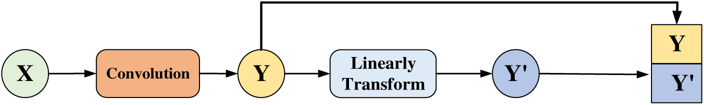
Figure 4: Internal structure of the Ghost module

Suppose the input features are h×w×m, where h and w represent the length and width of the input data, respectively, and m is the number of channels of the input; the output features are h ′×w ′×n, where h ′, w ′ are the length and width of the output data, respectively, n is the number of channels of the output, and k is the size of the convolution kernel. When the input data are convolved by the standard convolution, the number of parameters is n×k×k×m; when the input data are convolved by the Ghost convolution module, the number of parameters is n/s×k×k×m+(s−1)×n/s×k×k. Then, the compression ratio of the number of parameters of the Ghost module is s×m/(m+s−1)≈s. This paper cites the parameter setting of s=2 from the literature, which shows that when s=2, embedding the Ghost module in the network achieves the best network performance.

3  Malicious Code Family Detection Model Based on Ghost-DenseNet-SE

3.1 Malicious Code Visualization

The malicious code binary bit string can be divided into multiple substrings with a length of 8 bits. Each of these substrings is considered to be a pixel because these 8 bits can be regarded as unsigned integers in the range of 0–255, where 0 is black and 255 is white. We select three consecutive substrings, corresponding to the R, G, and B channels in the color image. That is, the first 8-bit string is transformed into the value of the R channel; the second 8-bit string, the value of the G channel; and the third 8-bit string, the value of the B channel. This operation is repeated so that all the data are selected. (The amount of data at the end of the last segment that is less than three strings is made up with 0 s.) Using this principle, the binary malicious code is then transformed into a one-dimensional vector of decimal numbers, with a fixed 256 line-width vector and a height that varies according to the file size. Eventually, the malicious code is interpreted as an RGB image, as shown in Fig. 5.

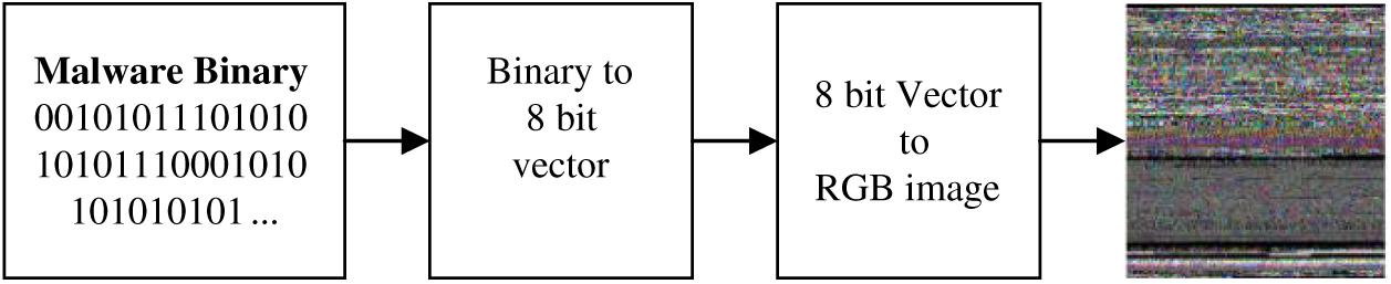
Figure 5: Malicious code visualization process

3.2 Model Construction

The Ghost-DenseNet-SeNet model proposed in this paper is used for detecting malicious code families. First, the malicious code is transformed into RGB images using malicious code visualization techniques. Then, the model is trained using the generated image dataset to classify and identify different families of malicious code. To address the challenges posed by the traditional CNNs, such as gradient disappearance and a sharp increase in the number of parameters with deeper and wider networks, we have adopted DenseNet as the backbone network. DenseNet encourages feature reuse and enables extraction of richer features from the malicious code images. To further enhance the model’s ability to accurately classify malicious code families, we incorporated the channel domain attention mechanism into DenseNet to obtain feature maps with more significant features. Finally, the Ghost module was employed to reconstruct the convolutional layer of the Dense Block, reducing the number of model parameters and facilitating deployment on mobile terminals with limited resources. The model structure is shown in Fig. 6.

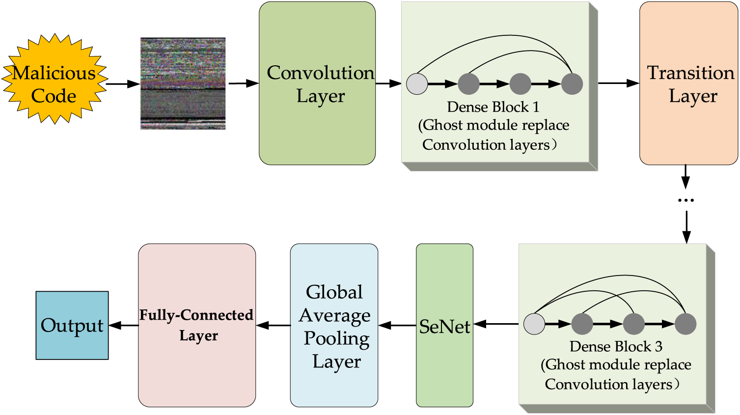
Figure 6: Malicious code detection model based on Ghost-DenseNet-SE

When the image dataset is fed into the model, the convolution operation is first applied, followed by the introduction of the first Dense Block. We utilize three such blocks, each containing 12 convolution operations with a size of 1×1 and 3×3. The output from the first 11 layers is utilized as the input for the 12th substructure. Transition layers are inserted between every two dense blocks, resulting in a total of two such layers. In this paper, the hyper-parameter θ in each Transition layer is set to 0.5, indicating that the number of output feature maps is halved compared to the original map.

By incorporating the SE module after the final Dense Block, we acquire a feature map that is rich in significant features. The module comprises two fully connected layers. The first fully connected layer is configured with a scaling factor ratio to compress the number of channels, which enhances computational efficiency. The specific values are optimized through experimental iterations. Subsequently, a global average pooling layer and a fully connected layer with 25 categories are appended to classify and detect malicious code families.

Due to the increase in model parameters resulting from the inclusion of the attention mechanism, the Dense Block is fine-tuned using the Ghost module, which replaces all 3×3 standard convolution layers except for the first convolution layer. The Ghost module employed in this paper comprises a point convolution and a 5×5 channel convolution. This configuration reduces the number of model parameters as the number of input channels varies. The greater the number of input channels, the more significant the reduction in the number of model parameters.

3.3 Model Training

The training process of CNNs involves two stages: Forward propagation and backward propagation. In the former, data is transmitted from the lower to higher levels, while in the latter, the error is transmitted from the higher to lower levels during training when the output from forward propagation does not match the expected result. The training process is depicted in Fig. 7 and follows these steps:

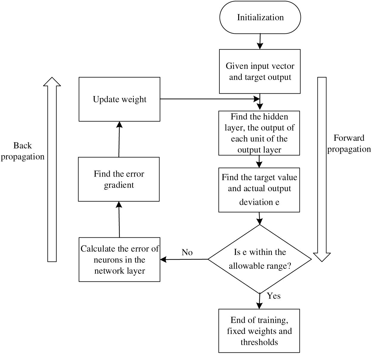
Figure 7: Model training process

1.    Initialize the network model’s weights.

2.    Input the image dataset and route it through the convolutional layer and the fully connected layer to obtain the output value.

3.    Identify the discrepancy between the network’s output value and the target value.

4.    If the error exceeds the desired value, it is relayed back to the network, and the errors in both the fully connected layer and convolutional layer are sequentially calculated. The gradients are then used to update the weights and offsets based on the detected error. If the error is equal to or less than the expected value, the training terminates.

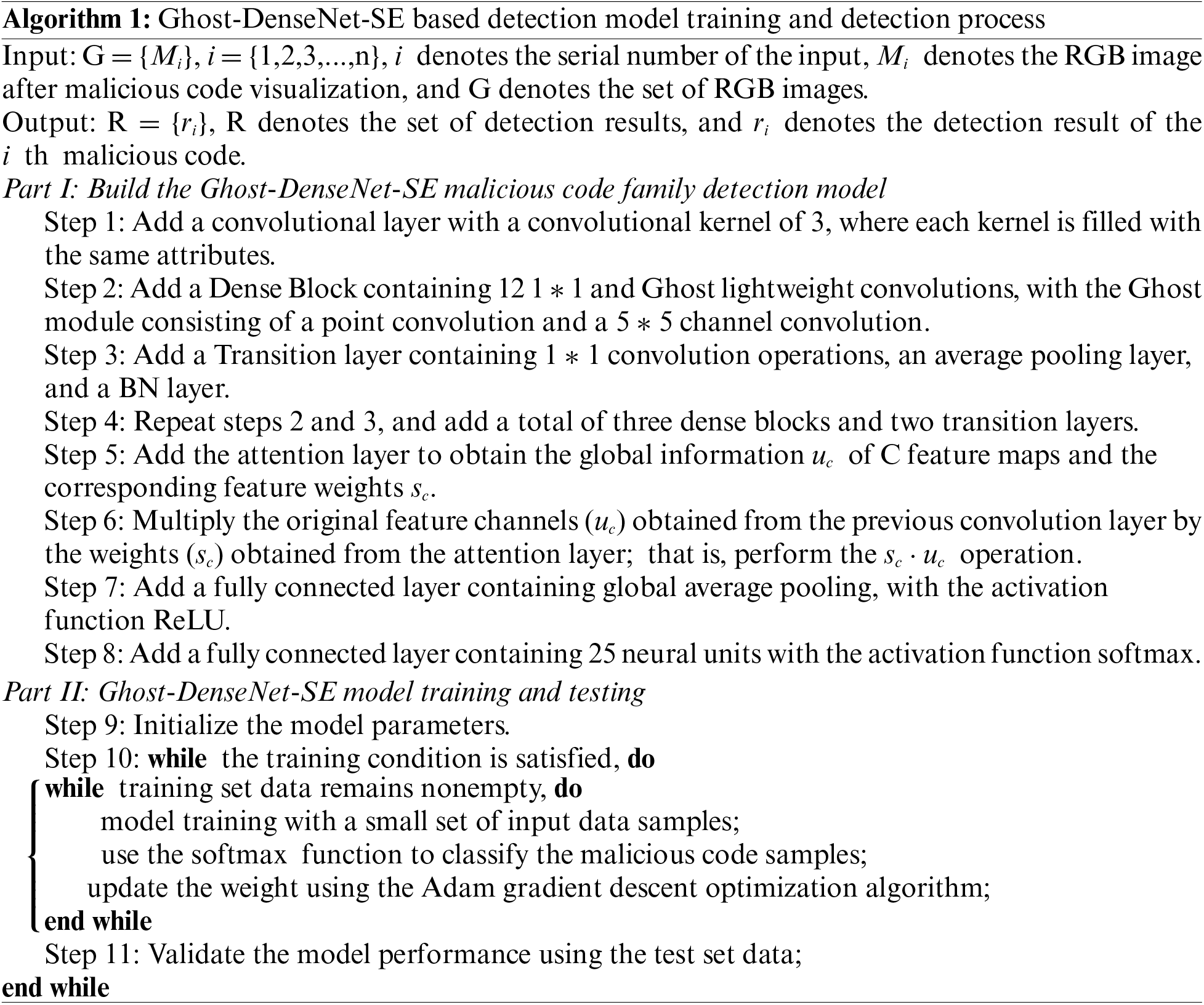
The relevant algorithms of the malicious code family detection model training and detection process in this paper are shown in Algorithm 1, which is divided into two parts.

4  Experimental Results and Analysis

4.1 Dataset

Because high-quality data are the key to deep learning, the acquisition of effective datasets is crucial. For this paper, we selected the public dataset Malimg, which enables the study of malicious code detection and obtaining malicious samples. This dataset includes 25 families of malicious samples, for a total of 9,339 samples. The specific sample types and their quantity distribution are shown in Fig. 8.

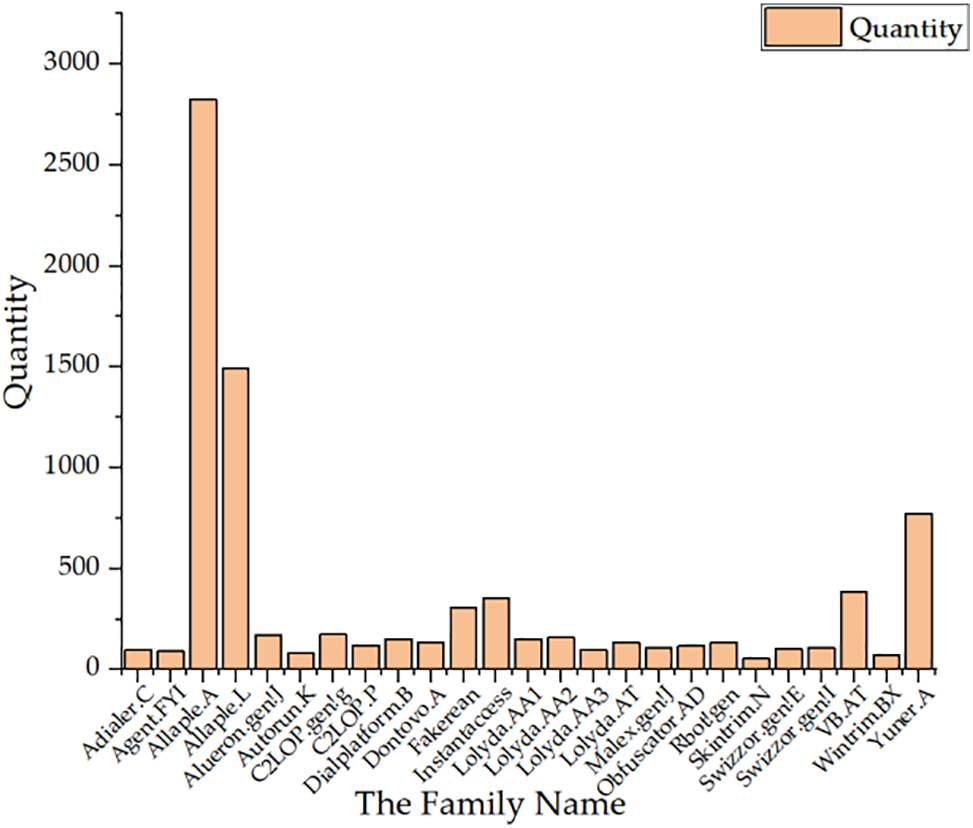
Figure 8: Malimg malicious code sample types and quantity distribution

The distribution of sample sizes in the Malimg dataset is highly unbalanced, with the smallest family, Skintrim.N, having only 80 samples, while the largest family, Allaple.A, has a whopping 2,949 samples. This distribution promotes over-fitting and compromises the model’s robustness and accuracy. Therefore, prior to the experiment, we employed down-sampling and data enhancement techniques to balance the dataset. Families with few samples were augmented using data enhancement techniques such as rotation and flipping, while families with a large number of samples were randomly subsampled using random down-sampling methods to match the sample sizes of families with fewer samples.

4.2 Data Preprocessing

CNNs require the input image size to be uniform, and malicious code binary executable files with varying sizes are converted into RGB images of different sizes. Therefore, the image must be processed into the same size image before being input into the neural network. The model used in this paper requires the input RGB image size to be 224×224. To ensure the integrity of the image texture information, we first used 0-byte padding on the border of the image to make it a square and then scaled it to 224×224. Fig. 9 shows sample images of some of the malicious code family binaries after preprocessing. From top to bottom, they are the Adialer.C family, VB.AT family, and Skintrim.N family. It can be seen from these image examples that malicious code of the same family has similarities in image texture, while the malicious code of different families exhibits differences in image texture.

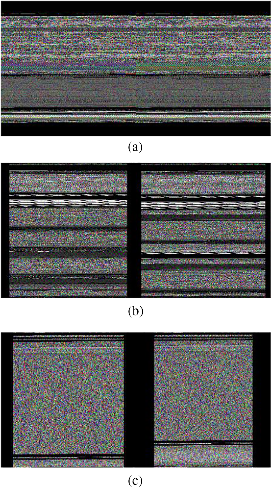
Figure 9: Part of the malicious code family image: (a) Adialer.C family; (b) VB.AT family; (c) Skintrim.N family

4.3 Evaluation Metrics

In the experimental process, five evaluation metrics were used to evaluate the proposed malicious code detection model: Accuracy, Precision, Recall, F1-score, and Loss.

TP: The fraction of positive samples correctly identified as positive by the model.

TN: The fraction of negative samples correctly identified as negative by the model.

FP: The fraction of negative samples incorrectly identified as positive by the model.

FN: The fraction of positive samples incorrectly identified as negative by the model.

1) Accuracy: The ratio of correctly predicted samples across all categories by the classifier, as illustrated below, to the total number of samples.

accuracy=TP+TNTP+FP+TN+FN(5)

2) Precision: For the prediction results, determine how many of the samples whose predictions were positive are truly positive samples, listed as below:

P=TPTP+FP(6)

3) Recall: Calculate the number of positive classes in the original sample that were correctly predicted, as demonstrated below:

R=TPTP+FN(7)

4) F1-score: A performance measurement constructed by combining precision and recall, with the goal of finding a certain balance between the two. The equation is given below:

F1=2×P×RP+R(8)

5) Loss: A measure of the distance between the predicted output probability and the actual output probability. The smaller the loss rate, the closer the two probability distributions. The equation is

Loss=−∑i=1i=qyi1log⁡yi1∧+yi2log⁡yi2∧+⋯+yidlog⁡yid∧(9)

where q is the number of samples, d is the number of sample categories, yid is the one-hot encoding value (0 or 1), and yid∧ is the output value of the softmax function output value (∑d=125yid∧).

4.4 Comparative Analysis

The experiment was conducted in a Centos7 system environment with a hardware configuration of an Intel Xeon Silver 4110 CPU @ 2.10 GHz, and a Quadro RTX 5000/Pcle/SSE2 GPU. The software included CUDA 11.0, PyCharm, using Python3.8, and the open-source deep learning training and testing frameworks of Keras 2.4.3 and TensorFlow 2.4.1.

4.4.1 Effect of Compression Ratio on Experiments

During the experiment, the dataset containing malicious code images was randomly partitioned into three sets: A training set, verification set, and test set, in a ratio of 8:1:1. The epoch was set to 100, and the batch size was set to 32. The experimental model employed DenseNet, a densely connected network, along with a channel domain attention mechanism. Settings such as the learning rate, compression ratio, loss function, and other parameters had an impact on the accuracy of malicious code detection. The model employed the cross-entropy loss function to quantify the discrepancy between actual and predicted values. It employed the Adam optimizer to optimize the network. The learning rate was set to 0.001, and the softmax function was used for classification purposes. The hyper-parameter ratio in the channel domain attention mechanism was determined through experiments to yield the most suitable value. The influence of the compression ratio on the performance of malicious code detection is summarized in Table 1.

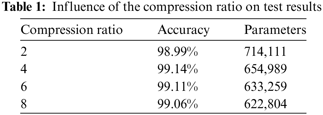
After conducting experiments, we arrived at a final hyper-parameter ratio of 4 after balancing the model’s accuracy and the number of parameters. The experimental results of the proposed method are presented in Fig. 10. As the number of tests increased, the accuracy and cross-entropy loss values converged to a certain value, indicating that the model gradually converged and became stable. Ultimately, the model achieved an impressive accuracy peak of 99.14%, with the corresponding loss value representing the optimal loss value for the model.

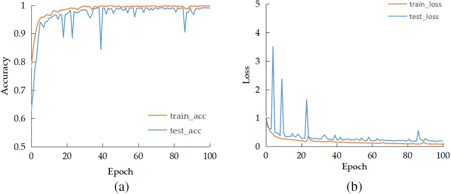
Figure 10: Ghost-DenseNet-SE detection model experiment results: (a) Accuracy; (b) Loss value

4.4.2 Model Performance Comparison

To further verify that the proposed DenseNet model incorporating the channel domain attention mechanism had high recognition accuracy for malicious code families, we compared it with the AlexNet detection model in [25] and the VGGNet detection model in [26]. Accuracy, recall, F1-score, and loss value were used as the evaluation metrics. The experimental results are shown in Table 2 and Fig. 11.

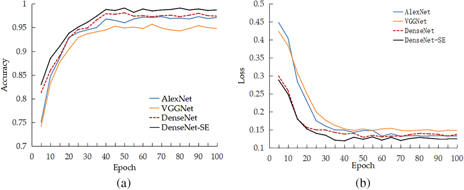
Figure 11: Comparison of experimental results of each model. (a) Accuracy of each model; (b) Loss value of each model

Based on Table 2 and Fig. 11, it is evident that the combination of the channel domain attention mechanism and DenseNet, when used as a malicious code family detection model, outperformed both AlexNet in [25] and VGGNet in [26] under identical experimental conditions. The model boasted an accuracy of 99.17%, which was 1.37% and 3.01% higher than its counterparts. Additionally, the model’s recall rate and F1-score were also superior to the models in the literature, indicating a more rapid convergence.

Furthermore, the DenseNet-SE model, which incorporated the attention mechanism, demonstrated a lower loss value, indicating that its detection results were closer to the true values. This was despite the fact that DenseNet alone had already achieved a higher accuracy rate than the other two models. This was due to the dense connections in Dense Block, which allowed for better feature propagation across all layers. By adding the attention mechanism to DenseNet, the accuracy rate increased by 0.97%, underscoring the ability of the mechanism to assign differential weights to channels and thereby extract more salient features.

In conclusion, the DenseNet-SE model excelled in terms of recognition accuracy and convergence speed for malicious code families. Apart from comparing the accuracy of each model, the experiment also compared the parameters of each model. Our optimization goal was to reduce the size of the model while enhancing detection accuracy. Table 3 presents the comparison results of the model parameters.

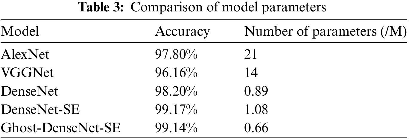
Based on Table 3, it is evident that the DenseNet network improved the accuracy of AlexNet by only 0.4%, but the model parameters were greatly reduced and the number of model parameters was also significantly reduced compared to VGGNet. This was due to the dense connections between the layers of DenseNet, which eliminated the need for some connections that would have been present in a traditional CNN. Incorporating the channel domain attention mechanism increased the number of model parameters. To address this, the lightweight Ghost module was used to reconstruct the convolutional layer of the Dense Block, reducing the number of parameters by 39% and compressing the model volume while only slightly decreasing the accuracy by 0.03%, which was considered negligible. The final comprehensive performance of the proposed malicious code family detection model combining the lightweight Ghost convolution, the densely connected network DenseNet, and the channel domain attention mechanism SE was better than that of the other detection models, demonstrating the effectiveness of the proposed method.

5  Conclusions

To address the limitations of existing malicious code family detection models, which suffer from low accuracy and excessive model parameters, we proposed a method based on Ghost-DenseNet-SE for detecting malicious code families. The model utilizes DenseNet as its backbone network, which utilizes a dense connection approach for each layer. This approach solves the problem of model degradation by deepening the network, reducing the number of model parameters, and enhancing feature transfer. To improve the model’s accuracy, we explored using the channel domain attention mechanism in computer vision, which assigns different weights to feature channels to enhance key information of malicious code RGB image texture features and improve the detection capability of the original model. To reduce model complexity, the lightweight Ghost module was used to reconstruct the convolutional layer of the Dense Block, reducing the number of parameters and compressing the model size. Experimental results demonstrate that the proposed method enhances the detection accuracy of malicious code families. The accuracy rate of 99.17% is higher than that achieved by other models, and it also reduced the number of parameters and model complexity. This is helpful for solving the problem of wasted resources in high-volume malicious code detection.

However, the proposed method still has some shortcomings, such as the memory overhead being too large during the model training. Follow-up work will further focus on ensuring the accuracy of model detection and calculation parameters while reducing the model memory overhead so that the method can be better deployed on mobile terminals with limited resources.

Although DenseNet has many advantages, it also has some drawbacks, such as higher memory usage. However, with continuous advancements in hardware devices and the emergence of optimization algorithms, these issues are gradually being addressed. Overall, DenseNet is a highly promising deep learning network architecture that deserves further research and application.

Acknowledgement: Not applicable.

Funding Statement: This research was funded by National Natural Science Foundation of China (under Grant No. 61905201).

Author Contributions: Study conception and design: X. L., M. Z.; data collection: Q. W.; analysis and interpretation of results: C. F., W. Z.; draft manuscript preparation: X. L. All authors reviewed the results and approved the final version of the manuscript.

Availability of Data and Materials: Data associated with this paper can be obtained by connecting to the corresponding author.

Conflicts of Interest: The authors declare that they have no conflicts of interest to report regarding the present study.

References

1. Beijing Rising Cyber Security Technology Co., Ltd., “2020 China cyber security report,” Inf. Secur. Res., vol. 7, no. 2, pp. 102–109, 2021. [Google Scholar]

2. A. Firdaus, N. B. Anuar, A. Karim, and M. F. A. Razak, “Discovering optimal features using static analysis and a genetic search based method for android malware detection,” Front. Inf. Technol. Electron. Eng., vol. 19, no. 6, pp. 712–736, 2018. doi: 10.1631/FITEE.1601491. [Google Scholar] [CrossRef]

3. P. Yan and Z. Yan, “A survey on dynamic mobile malware detection,” Software Qual. J., vol. 26, no. 3, pp. 891–919, 2018. doi: 10.1007/s11219-017-9368-4. [Google Scholar] [CrossRef]

4. J. Gu et al., “Recent advances in convolutional neural networks,” Pattern Recognit., vol. 77, pp. 354–377, 2018. doi: 10.1016/j.patcog.2017.10.013. [Google Scholar] [CrossRef]

5. Z. Cui, F. Xue, X. Cai, Y. Cao, and G. Wang, “Detection of malicious code variants based on deep learning,” IEEE Trans. Industr. Inform., vol. 14, no. 7, pp. 3187–3196, 2018. doi: 10.1109/TII.2018.2822680. [Google Scholar] [CrossRef]

6. G. Wang, T. Lu, H. Yin, and J. Zhang, “Malicious code family detection technology based on CNN-BiLSTM,” Comput. Eng. Appl., vol. 56, no. 24, pp. 72–77, 2020. [Google Scholar]

7. J. Zhao, S. Zhang, B. Liu, and B. Cui, “Malware detection using machine learning based on the combination of dynamic and static features,” in 27th Int. Conf. Comput. Commun. Netw. ICCCN, Hangzhou, China, 2018, pp. 1–6. [Google Scholar]

8. P. Yang, Y. Pan, P. Jia, and L. Liu, “Malware detection based on word embedding features of assembly instruction,” J. Inform. Secur. Res., vol. 6, no. 2, pp. 113–121, 2020. [Google Scholar]

9. E. Raff, J. Sylvester, and C. Nicholas, “Learning the PE header, malware detection with minimal domain knowledge,” in Proc. 10th ACM Workshop Artif. Intell. Secur., New York, NY, USA, Nov. 2017, pp. 121–132. [Google Scholar]

10. S. Zhao, X. Ma, W. Zou, and B. Bai, “DeepCG: Classifying metamorphic malware through deep learning of call graphs,” in Secur. Priv. Commun. Netw. Secur. 2019 Lect. Notes Inst. Comput. Sci. Soc. Inform. Telecommun. Eng., Cham, 2019, vol. 304, pp. 171–190. [Google Scholar]

11. I. Santos, F. Brezo, X. Ugarte-Pedrero, and P. G. Bringas, “Opcode sequences as representation of executables for data-mining-based unknown malware detection,” Inform. Sci., vol. 231, pp. 64–82, 2013. [Google Scholar]

12. B. Kang, S. Y. Yerima, K. Mclaughlin, and S. Sezer, “N-opcode analysis for Android malware classification and categorization,” in Int. Conf. Cyber Secur. Prot. Digit. Serv. Cyber Secur., London, UK, 2016, pp. 1–7. [Google Scholar]

13. R. Pascanu, J. W. Stokes, H. Sanossian, M. Marinescu, and A. Thomas, “Malware classification with recurrent networks,” in IEEE Int. Conf. Acoust. Speech Signal Process. (ICASSP), South Brisbane, QLD, Australia, 2015, pp. 1916–1920. [Google Scholar]

14. I. Kwon and E. G. Im, “Extracting the representative API call patterns of malware families using recurrent neural network,” in Proc. Int. Conf. Res. Adapt. Converg. Syst., New York, NY, USA, Sep. 2017, pp. 202–207. [Google Scholar]

15. T. Messay-Kebede, B. N. Narayanan, and O. Djaneye-Boundjou, “Combination of traditional and deep learning based architectures to overcome class imbalance and its application to malware classification,” in NAECON 2018—IEEE Natl. Aerosp. Electron. Conf., Dayton, OH, USA, Jul. 2018, pp. 73–77. [Google Scholar]

16. D. Gibert, C. Mateu, and J. Planes, “Orthrus: A bimodal learning architecture for malware classification,” in Int. Jt. Conf. Neural Netw. (IJCNN), Glasgow, UK, 2020, pp. 1–8. [Google Scholar]

17. J. Yan, Y. Qi, and Q. Rao, “Detecting malware with an ensemble method based on deep neural network,” Secur. Commun. Netw., vol. 2018, pp. e7247095, 2018. doi: 10.1155/2018/7247095. [Google Scholar] [CrossRef]

18. B. N. Narayanan and V. S. P. Davuluru, “Ensemble malware classification system using deep neural networks,” Electron., vol. 9, no. 5, pp. 721, 2020. doi: 10.3390/electronics9050721. [Google Scholar] [CrossRef]

19. M. Ahmadi, D. Ulyanov, S. Semenov, M. Trofimov, and G. Giacinto, “Novel feature extraction, selection and fusion for effective malware family classification,” in Proc. Sixth ACM Conf. Data Appl. Secur. Priv., New York, NY, USA, Mar. 2016, pp. 183–194. [Google Scholar]

20. Y. Zhang, Q. Huang, X. Ma, Z. Yang, and J. Jiang, “Using multi-features and ensemble learning method for imbalanced malware classification,” in IEEE Trust, Tianjin, China, Aug. 2016, pp. 965–973. [Google Scholar]

21. A. Krizhevsky, I. Sutskever, and G. E. Hinton, “ImageNet classification with deep convolutional neural networks,” Commun. ACM, vol. 60, no. 6, pp. 84–90, 2017. [Google Scholar]

22. K. Simonyan and A. Zisserman, “Very deep convolutional networks for large-scale image recognition,” arXiv:1409.1556, 2015. [Google Scholar]

23. C. Szegedy, W. Liu, Y. Jia, P. Sermanet, and S. Reed, “Going deeper with convolutions,” in IEEE Conf. Comput. Vis. Pattern Recognit. (CVPR), Jun. 2015, pp. 1–9. [Google Scholar]

24. K. He, X. Zhang, S. Ren, and J. Sun, “Deep residual learning for image recognition,” in IEEE Conf. Comput. Vis. Pattern Recognit. (CVPR), Las Vegas, NV, USA, 2016, pp. 770–778. [Google Scholar]

25. K. Jiang et al., “Malicious code detection based on multi-channel image deep learning,” J. Comput. Appl., 4, pp. 1142–1147, 2021. [Google Scholar]

26. B. Wang, H. Cai, and Y. Su, “Classification of malicious code variants based on VGGNet,” J. Comput. Appl., vol. 40, no. 1, pp. 162, 2020. doi: 10.11772/j.issn.1001-9081.2019050953. [Google Scholar] [CrossRef]

27. G. Huang, Z. Liu, L. van der Maaten and K. Q. Weinberger, “Densely connected convolutional networks,” in IEEE Conf. Comput. Vis. Pattern Recognit. CVPR, Honolulu, HI, USA, 2017, pp. 2261–2269. [Google Scholar]

28. F. Wang et al., “Residual attention network for image classification,” in IEEE Conf. Comput. Vis. Pattern Recognit. (CVPR), Honolulu, HI, USA, 2017, pp. 6450–6458. [Google Scholar]

29. J. Hu, L. Shen, and G. Sun, “Squeeze-and-excitation networks,” in IEEECVF Conf. Comput. Vis. Pattern Recognit. (CVPR), Salt Lake City, UT, USA, 2018, pp. 7132–7141. [Google Scholar]

30. K. Han, Y. Wang, Q. Tian, J. Guo, C. Xu and C. Xu, “GhostNet: More features from cheap operations,” in IEEECVF Conf. Comput. Vis. Pattern Recognit. (CVPR), Seattle, WA, USA, 2020, pp. 1577–1586. [Google Scholar]