Multiple Perspective of Multipredictor Mechanism and Multihistogram Modification for High-Fidelity Reversible Data Hiding

1  Introduction

With the rapid development of big data and Internet technologies, information security has become an important issue. Information security is a broad topic that includes protecting digital information from unauthorized access or disclosure. One technique used in information security is watermarking, which allows for the embedding of specific information to identify copyright or for auditing purposes in digital media such as images and text files. Complementary to watermarking methods are watermarking attack methods [1,2], which are used to attempt to remove or alter the embedded information in order to make it difficult or impossible to trace the usage of the media. The study of these attack methods can help to inform the development of a more robust watermarking technology. Image encryption [3] is another useful tool for information security as it involves encrypting image files so that they can only be decrypted and viewed with the correct key. In addition, image description is the process of processing an image so that lost information can be recovered or reconstructed or the quality of the image can be improved [4–6]. All of these techniques can be used in information security and can help protect the integrity and security of digital information. Data hiding, an important branch of information security, can achieve the goals of copyright protection, secret communication, etc., via embedding secret data into cover media such as images, videos, and audio in a perceptible way. Nevertheless, data hiding can also cause irreversible damage to the cover media while embedding the secret data. Reversible data hiding (RDH) [7–10], as a derivative technique of data hiding, is characterized by the ability to recover the cover media losslessly after the correct extraction of the secret data. Currently, RDH is widely used in medical, military, and e-commerce fields, which do not allow reversible damage to the cover media.

After decades of research, many effective RDH algorithms have been proposed [11–14]. Currently, RDH schemes can be classified into four categories: (1) RDH based on the spatial domain [15–19]; (2) RDH based on the encrypted domain [20–24]; (3) RDH based on the transform domain [25–27]; and (4) RDH based on the compressed domain [28,29]. Further, the proposed scheme is focused on the first category of RDH. Thus far, many excellent spatial domain-based RDH schemes have been proposed, such as histogram shifting (HS) [7], difference expansion (DE) [30,31], prediction error expansion (PEE) [15–19], etc. The concept of HS, which refers to histogram manipulation in which the peak bins are used to carry the secret data, while the remaining bins are shifted, was first introduced by Ni et al. [7]; while Tian et al. [30] first proposed the DE-based scheme, which expands the difference between adjacent pixels; then, a vacant least-significant-bit (LSB) is created for the data embedding. As an extension of DE, PEE was first proposed by Thodi and Rodriguez [32]. Unlike DE, which embeds the secret data by expanding the difference between neighboring pixels, PEE exploits the difference between a pixel’s intensity and its predicted value for embedding. Since the accuracy of prediction directly corresponds to the distortion of the cover image, research has focused on how to improve the accuracy of prediction [33–35]. PEE is an effective and extensively exploited scheme, as it exploits the redundancy of the cover image and constructs a sharper prediction error histogram (PEH). Note that the performance of PEE has been continuously enhanced by many works, such as through precise prediction mechanisms [11,13,17,36], adaptive 1D PEH modifications [37], 2D PEH modifications [16,18], and so on.

According to the principle of PEE, the prediction scheme involves the predicted pixel and predicted value, which determines the distribution of prediction errors. In 2009, Sachnev et al. [38] proposed a prediction mechanism, which predicts a central pixel by averaging its four neighboring pixels. Thus far, many PEE schemes have used the rhombus prediction mechanism. To further improve PEE performance, Li et al. [39] proposed a novel PEE scheme called “pixel value ordering” (PVO), which aims to predict the maximum and minimum values using the second-largest and second-smallest values in each image block, respectively. PVO has been verified to achieve low distortion under low payload. Afterward, a large number of PVO-based schemes were proposed. In [40], PVO was extended to PVO-k by modifying the k largest/smallest pixels of each image block. In [41], Peng et al. added the concept of the relative position of pixels to PVO and proposed improved PVO (IPVO) with better performance. After that, Wang et al. [42] used a strategy to determine the block size adaptively, which increased the embedding performance. In addition, Qu et al. [43] proposed a pixel-based PVO scheme that abandons the use of the image block, where each pixel is predicted by its sorted context.

The aforementioned PVO-based schemes are well established, but such schemes only perform well in a smooth image area. There should be a more efficient solution in the complex image areas to reduce distortion. In [44], Ma et al. proposed a multipredictor scheme to predict a pixel in different methods and select the most appropriate predicted value. This scheme is good at reducing the distortion of the complex regions; however, the conditions of data embedding are too harsh, which leads to the low hiding capacity of the algorithm as well. To ensure the embedding volume and image quality, we propose a novel RDH, which combines the advantages of the multipredictor mechanism and multihistogram technique. First, we improve the prediction accuracy by combining IPVO and the median edge detector (MED) prediction mechanism [45]. To further enhance the performance of the proposed scheme, a new complexity metric is proposed to skip the complex regions in the cover image. Finally, we use the multihistogram technique to select the optimal embedding bin in each subhistogram. Experimental results show that the proposed scheme achieves an advantage in fidelity over a series of state-of-the-art schemes with moderate capacity. The main contributions of this paper are summarized as follows:

1.    Novel multipredictor mechanism. In combining IPVO and MED, a novel multipredictor mechanism is proposed to better improve prediction accuracy.

2.    Adaptive local complexity metric. The proposed complexity metric can help filter the appropriate regions in the cover image and the generation of multiple histograms.

3.    Incorporation of multihistogram and optimal embedding bin selection. How the grouping backpack model is applied to the selection of optimal embedding bins is studied.

The rest of this paper is organized as follows. Section 2 introduces the preliminary works. In Section 3, we describe the proposed scheme step by step. In Section 4, the experimental results of the proposed scheme are provided. Finally, conclusions and prospects are presented in Section 5.

2  Preliminary Works

In this section, the basic principle of the PVO-based schemes is first reviewed in Subsections 2.1 and 2.2. Then, the technique of MED prediction is introduced in detail, which is an important part of the proposed scheme. Next, because the concept of the multipredictor mechanism (MPM) is applied in the proposed scheme, we also give a brief introduction to the MPM in Subsection 2.4.

2.1 PVO-Based PEE

Li et al. [39] first designed a PVO scheme by using the conventional PEE. In their scheme, the original image is first divided into mutually exclusive blocks. Assume that each block contains l pixels, pixels are collected as {p1,p2,…,pl} and sorted in ascending order to obtain {pσ(1),pσ(2),…,pσ(l)}, where σ:{1,2,…,l}→{1,2,…,l} is the one-to-one mapping, σ(i)<σ(j) if pσ(i)=pσ(j) and i<j. Then, the prediction errors dmax and dmin are calculated as

{dmax=pσ(l)−pσ(l−1)dmin=pσ(1)−pσ(2).(1)

Then, the prediction errors are modified to

dmax={dmax,ifdmax=0dmax+m,ifdmax=1dmax+1,ifdmax>1,(2)

dmin={dmin,ifdmin=0dmin−m,ifdmin=−1dmin−1,ifdmin<−1,(3)

where m∈{0,1} is a secret bit, and pσ(l) and pσ(1) are accordingly enlarged and decreased, respectively.

2.2 IPVO-Based PEE

Although PVO-based PEE is effective, it has an obvious drawback. According to Eqs. (2) and (3), prediction-error valued 0 is excluded for data embedding, which wastes the embedding capacity of a large number of the smooth block. To solve this problem, the concept of relative location is utilized in [36] by renewing the prediction-errors as

{dmax=pu−pvdmin=px−py,(4)

where u=min(σ(l−1),σ(l)), v=max(σ(l−1),σ(l)), and x=min(σ(1),σ(2)), v=max(σ(1),σ(2)).

Then, the maximum and minimum pixels pσ(l) and pσ(1) are modified to p~σ(l) and p~σ(1), respectively, by

p~σ(l)={pσ(l)+m,if  dmax∈{0,1}pσ(l)+1,others;(5)

p~σ(1)={pσ(1)−m,if  dmin∈{0,1}pσ(1)−1,others.(6)

2.3 Median-Edge Detector Prediction

Generally speaking, IPVO-based schemes can be regarded as a prediction method that uses the second-largest and second-smallest values within a block to predict the largest and smallest values. However, this prediction method only performs well on smooth blocks.

Weinberger et al. [45] first proposed the median-edge detector prediction (MED), which can offer more accurate predictions even in normal image blocks. As shown in Fig. 1, MED applies the edge rule to predict the current pixel x based on the values of the context pixels a,b, and c by

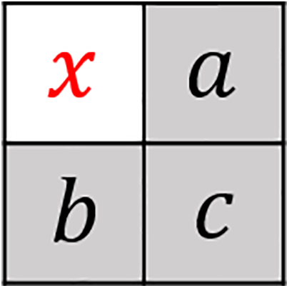
Figure 1: Data structure of median-edge detector prediction (MED)

x~={min(a,b),if   c≥max(a,b)max(a,b),if  c≤min(a,b)a+b−c,others,(7)

where x~ is the output of the predicted value.

The prediction error e can be calculated as e=x−x~. Then, the process of data embedding can be carried out according to the value of e.

2.4 Multipredictor Mechanism

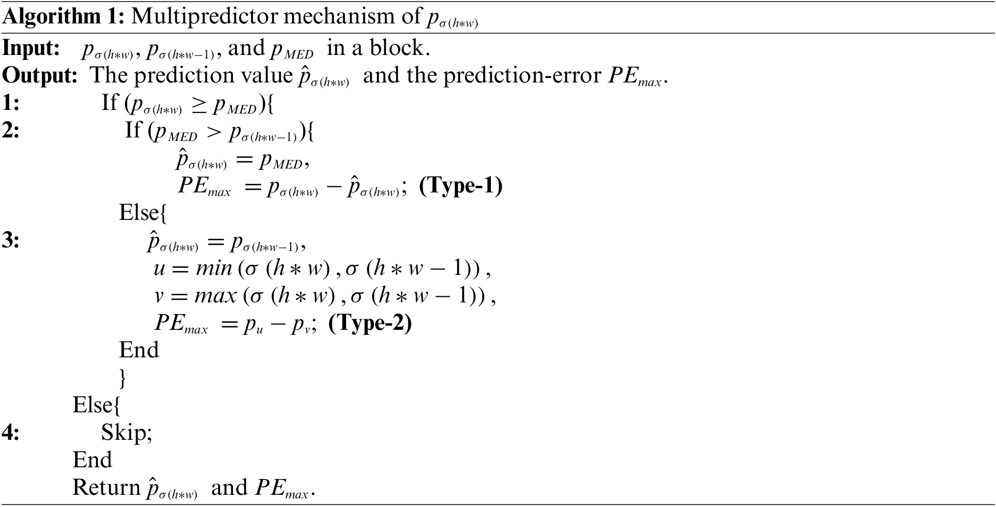
Using only one prediction rule does not apply to all blocks in the image. To obtain higher prediction accuracy, Ma et al. [44] proposed a multiprediction mechanism, which used k different predictors to predict pixel p. After obtaining k prediction values {p^1,p^2,…,p^k}, the maximum and minimum predicted values p^min=min(p^1,p^2,…,p^k) and p^max=max(p^1,p^2,…,p^k) is utilized to calculate an optimal prediction value p~ as

p~={p^min,if  p^min=p^max(Type 1)p^min,if  p≤p^min(Type 2)p^max,if  p≥p^max(Type 3)∅,others (Type 4),(8)

where ∅ means there is no predicted value for the current pixel p.

Similarly, the prediction errore can be calculated as e=p−p~ for Type 1, Type 2, and Type 3.

For Type 1, new prediction error e~ is calculated as

e~={e+m,if   e=0e+1,if   e>0e−m,if  e=−1e−1,if  e<−1.(9)

For Type 2 and Type 3, new prediction error e~ is calculated, respectively, as

e~={e−m,if   e=0e−1,if  e<0.(10)

e~={e+m,if  e=0e+1,if  e>0.(11)

Finally, the new embedded pixel p′ is updated by p′=p~+e~.

3  Proposed Scheme

This section presents an adaptive RDH algorithm using a multipredictor mechanism combined with the multihistogram technique. First, we describe and analyze the novel multipredictor mechanism combining IPVO and MED. Then, we propose an adaptive local complexity metric. After that, we incorporate the multihistogram technique. Finally, we present implementation details for the proposed scheme.

3.1 Multipredictor Mechanism Combining IPVO and MED

Assuming the original gray-scale image is divided into K nonoverlapping blocks of size h∗w, and we only take the largest pixel in the block as an example, the embedding process of the smallest pixel is similar to that of the largest pixel. In the first step, as in IPVO, we sort the pixels {p1,p2,…,ph∗w} within the current block to obtain {pσ(1),pσ(2),…,pσ(h∗w)}. Second, we find the three context pixels {a,b,c} of pσ(h∗w). Then, we utilize MED to obtain the predicted value pMED of pσ(h∗w). Finally, the multipredictor mechanism combines IPVO and MED for pσ(h∗w) as shown in Algorithm 1.

If PEmax belongs to Type-1, to embed the secret data via PEE, PEmax is modified to

PE~max={PEmax+m,if PEmax=0PEmax+1,if PEmax>0.(12)

If PEmax belongs to Type-2, PEmax is modified to

PE~max={PEmax+m,if PEmax=1PEmax+1,if PEmax>1PEmax−m,ifPEmax=0PEmax−1,ifPEmax<0.(13)

Finally, the maximum pixel pσ(h∗w) is modified to pσ(h∗w)′=p^σ(h∗w)+|PE~max|.

As shown in Fig. 2, there are three types of relationship among pMED, pσ(h∗w), and pσ(h∗w−1). Provided the value of pMED falls into Region 1, then the PEmax will belong to the Type-2 case in Algorithm 1. Provided the value of pMED falls into Region 2, then the PEmax will belong to the Type-1 case in Algorithm 1, and the distribution of PEmax can be sharper. Finally, when the value of pMED falls into Region 3, the embedding process will simply be avoided.

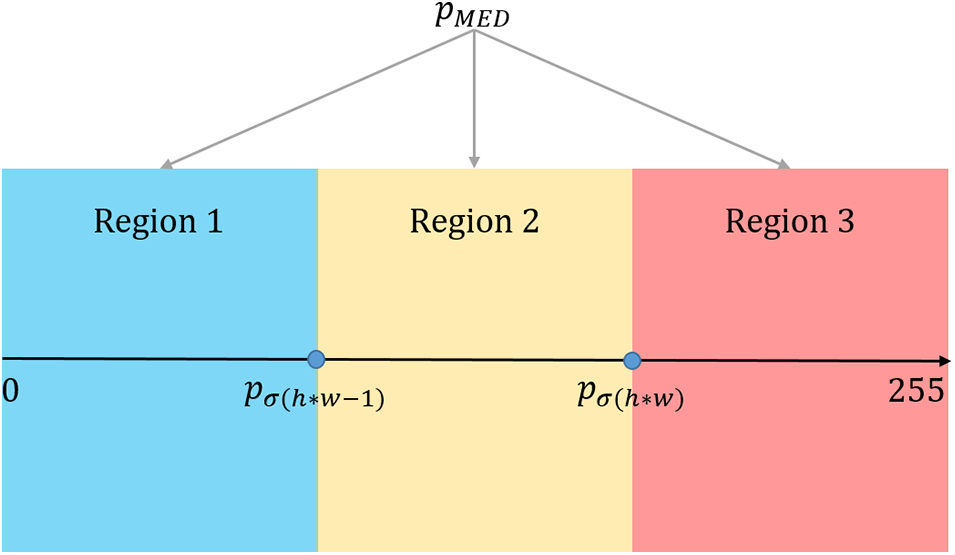
Figure 2: Three types of relationships among pMED, pσ(h∗w), and pσ(h∗w−1)

When performing the embedding process, the secret data are first embedded in the largest pixel of each block in index order. When the largest pixel is used up, the secret data are then embedded in the smallest pixel of each block according to the same index order. The previous schemes [11,13,40,41] used the maximum and minimum pixels of each block simultaneously, leading to two problems: (1) when the value of the largest pixel changes, it may affect the prediction value of the smallest pixel, making the smallest pixel unavailable; (2) when the largest pixel within a block is shifted, then the texture around the current block is complex. At this time, it is highly probable that the smallest pixel will be shifted in the embedding process. Provided we divide the maximum and minimum pixels in the block into two layers to embed the secret data, when the amount of data to be embedded is small, we can protect the partial smallest pixels from being shifted, which can improve image quality.

3.2 Adaptive Local Complexity Metric

Obviously, the above multipredictor mechanism is not suitable for all types of image blocks. A more accurate prediction depends not only on the texture feature of the current image block but also on the complexity of the three neighboring pixels around the predicted pixel. Thus, the block-based complexity measure proposed by Peng et al. [41], i.e., Cb=pσ(h×w−1)−pσ(2), is not well-suited to the proposed scheme. To solve this problem, we introduce a neighbor-based complexity metric Cn, which is defined as

Cn=(|a−b|+|a−c|+|b−c|)/3.(14)

When embedding a small payload, the image block size is relatively large, for example, 5×5 or 5×4; thus, the computation of Cb can cover more pixels and is thus more representative of the complexity around the predicted pixel. As the embedding payload increases, the size of the image block decrease to improve the image’s embedding capacity. In this case, Cb cannot reflect the complexity around the predicted pixel. Thus, we propose a novel adaptive local complexity metric Ca to classify the image block

Ca=μ×Cb+(1−μ)×Cn,(μ=max(h,w)5),(15)

where μ is a sensitivity factor. Since the maximum value of w and h is 5, the denominator of μ is set to 5. As the image block becomes smaller, so does the value of μ.

3.3 Adaptive Multiple Histograms Generation and Optimal Embedding Bins Selections

It is well known that the objective of the RDH scheme is to achieve a certain payload while minimizing cover image distortion. A feasible way to accomplish this is to divide the predicted pixels into multiple classes according to our complexity metric and design different embedding mechanisms for each class of predicted pixels to minimize image distortion. First, we set a threshold T1 for the complexity metric Ca. After that, we divide T1 into n=⌈T1⌉ equal intervals. Thus, all the predicted pixels with a complexity less than T1 can be classified into one of the classes in n. For example, provided we set T1=6.2, then n=7; there is also a predicted pixel with a complexity of 6.1, which will be classified in the 7th class. Finally, we calculate and count the prediction errors in each class separately to form n subhistograms.

For the one histogram shifting algorithm, brute force search is one of the most frequently used search algorithms, which searches for the best embedding bins by traversing all possible combinations thereof. However, for multiple histograms, many possible combinations of embedding bins can achieve a certain payload. Therefore, it is time-consuming to iterate through all possible combinations one by one.

Searching for the optimal embedding bins of multiple histograms can be considered a combinatorial optimization problem. Thus, we transform the above search problem into a typical grouped knapsack problem.

To simplify the grouped knapsack problem, we count only the prediction errors using IPVO. First, we divide a cover image into two layers and calculate all the bins suitable for pσ(h×w) in each block; then, we calculate suitable bins for pσ(1) in each block after all the pσ(h×w) has been used. We choose one embedding bin pair (Plk,Prk), where Plk≤0 and Prk>0, for the kth subhistogram hk, where k∈{1,2,…,n}. Thus, n subhistograms can generate 2n parts. According to the histogram shifting technique, if Prk is selected as the embedding bin, all bins greater than Prk in the kth subhistogram should be shifted 1 unit to the right; similarly, if Plk is selected as the embedding bin, all bins smaller than Plk in the kth subhistogram should be shifted 1 unit to the left. The sum of hk(Plk) and hk(Prk) is equivalent to the embedding capacity. Thus, the target mathematical model of embedding capacity and distortion is defined as

{min∑k=1n⁡(∑e<Plk⁡hk(e)+∑e>Prk⁡hk(e)+12hk(Plk)+12hk(Prk))S.T.∑k=1n⁡(hk(Plk)+12hk(Prk))≥eclayer,(16)

where hk(e) represents the occurring frequency of prediction error e in hk, and ec represents the given payload in the current layer. Since we only calculate suitable bins for the prediction error of Type 2, the ec is calculated as

eclayer=EC2−num(Type1(PE=0))layer,(17)

where EC is the total given payload. Provided the embedding capacity of the first and second layers does not reach eclayer, then the bins with the maximum embedding capacity are selected for the first layer.

Next, we transform Eq. (16) into a grouped knapsack problem. We replace the embedding capacity and embedding distortion with the weight and value of the commodity, respectively. This establishes a one-to-one relationship between the parameters in Eq. (16) and the grouped knapsack problem. For example, 2n parts of n subhistograms correspond to 2n categories of the commodity. Since we only select one bin for embedding in each category, provided the number of commodity samples in the αth category is ηα, the target of the grouped knapsack problem becomes

{min∑α=12n⁡∑β=1ηα⁡Dα,β×λα,βS.T.∑α=12n⁡∑βηα⁡Vα,β×λα,β≥EC,(18)

where Dα,β and Vα,β are the weight and value of the βth sample in the αth category, respectively. It is worth mentioning that λα,β is a vector of size 1×ηα; only the βth position is 1, while the rest are 0. This indicates that only the βth sample in the αthcategory is chosen for embedding.

For example, provided the threshold of the complexity metric is set to 5.9, then all the pσ(h∗w) predicted by IPVO are divided into six classes, and each class constructs one subhistogram of prediction error. Correspondingly, the search space is divided into 6×2=12 categories of the commodity. In order to save search time, we set a hyperparameter τ to specify the number of samples in each category. If τ is set to 5, then each category includes five samples {−4, −3, −2, −1, 0} or {1, 2, 3, 4, 5}, and all embedding bins can be found in these 10 samples.

3.4 Implementation of the Proposed Scheme

To better demonstrate the process of data embedding, two types of examples are given in Fig. 3. Here, suppose that the block size is 3×3, threshold T  of complexity metric is 5.9, the secret message m=1, and the embedding bins for the current sub-histogram is {0,1}. As shown in Fig. 3a, when the PEmax belongs to Type-1, the embedding process is performed according to Eq. (12); when the PEmax belongs to Type-2, as shown in Fig. 3b, the complexity of the region where pσ(h∗w) is located is first calculated; then, the corresponding sub-histogram is selected according to the complexity. Finally, the secret data are embedded according to the bins selected by the current sub-histogram.

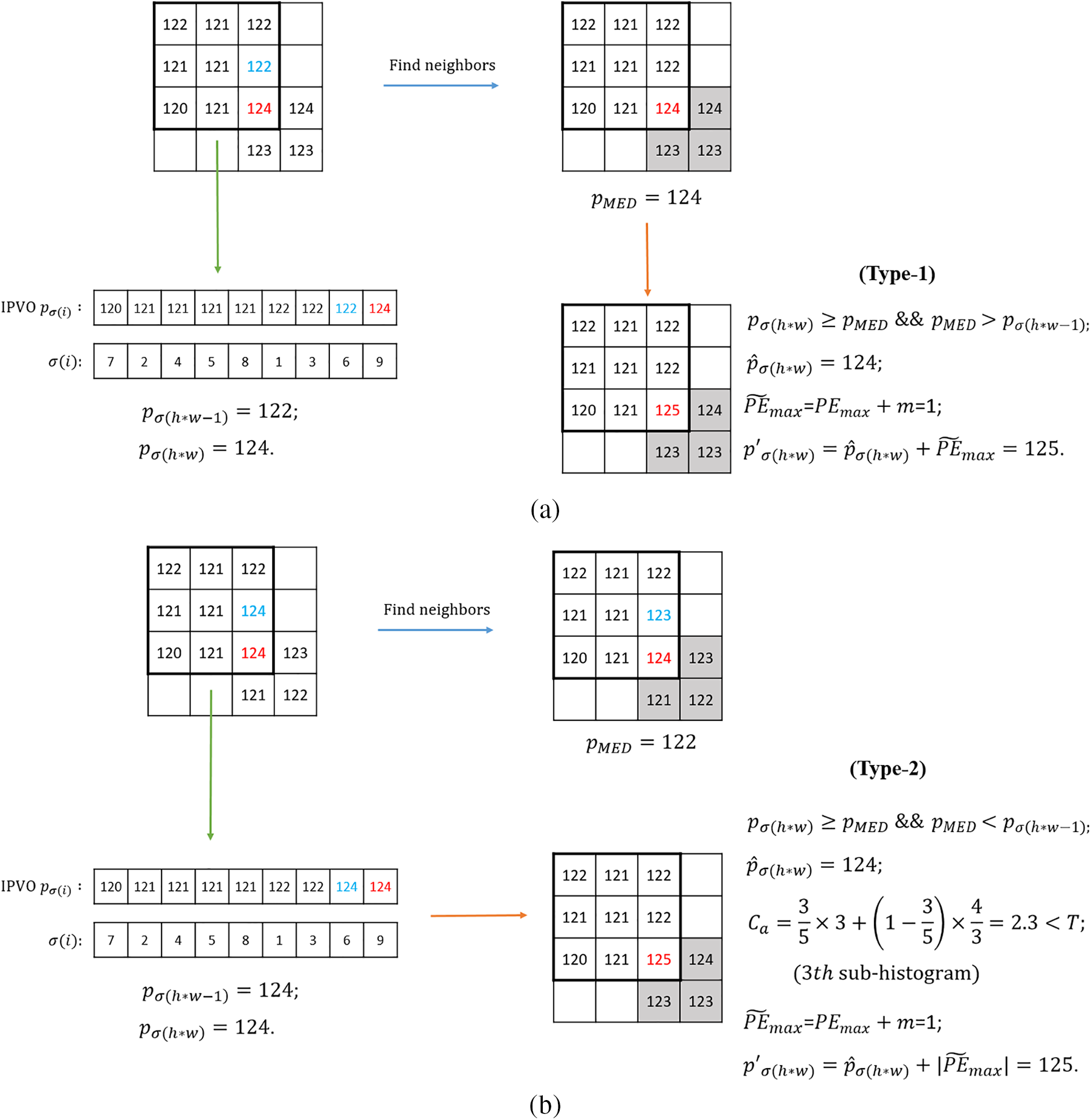
Figure 3: Examples of embedding process

Now, we will elaborate on the processes of data embedding and data extraction. To solve the pixel overflow/underflow problem, we utilize a location map to ensure that pixels in the stego image do not exceed the range [0,255]. The value 255 is modified to 254, and the value 0 is modified to 1. Meanwhile, the location of each modified pixel is recorded as 1 on the location map, while those that are not modified are recorded as 0. Then, we losslessly compress the location map using arithmetic compression to reduce its length.

Besides the location map, some auxiliary information also needs to be recorded:

◼ The size h and w of block (3×3=9 bits).

◼ The threshold T of complexity; the first 8 bits record the integer bits; the last 4 bits record the fractional bits (8+4=12 bits).

◼ All total embedding optimal bins of two layers (2×3×2n=12n bits).

◼ End positions of two layers (2×log2⁡(512×512)=36 bits).

◼ The length of the compressed location map (log2⁡(512×512)=18 bits).

◼ The compressed location map (Lclm bits).

The auxiliary information is embedded in the last two rows of the cover image through LSB replacement so that the extractor can access this information and thus extract the secret data correctly and recover the cover image losslessly. Next, the complete process of data embedding occurs as follows.

Data Embedding Process

Step 1. Construct the location map to prevent the pixel overflow/underflow problem. Empty the LSBs of pixels in the first two rows. Add the replaced LSBs to the head of the payload.

Step 2. Divide the cover image into mutually exclusive blocks of size h∗w. Generate n sub-histograms according to the threshold of complexity T; then, divide the Type-2 prediction errors in the first layer into the respective sub-histograms.

Step 3. Select the appropriate bins for each sub-histogram of the first layer.

Step 4. Embed the secret data in the first layer using the proposed multipredictor mechanism and the selected bins.

Step 5. Embed the secret data for the second layer as in Steps 3 and 4.

Step 6. Record the auxiliary information into the LSBs of the pixels of the first two rows. Finally, generate the stego image.

For data extraction and image recovery, all operations are inversions of the embedding process, i.e., we process the second layer and then the first layer; the blocks are processed in the inverse scanning order of data embedding. The detailed data extraction process is as follows.

Data Extracting Process

Step 1. Extract and decode the auxiliary information from the LSBs of the pixels in the first two rows.

Step 2. Divide the stego image into mutually exclusive blocks of size h∗w. Extract the secret data and restore the second layer from its end position. After that, process the first layer similarly.

Step 3. Recover the pixels of the first two rows using the header of the extracted secret data.

Step 4. Decompress the map and use it to losslessly restore the original cover image.

4  Experiment Results

In this section, we perform some experiments to verify the performance of the proposed scheme. Six standard gray-scale images are used as test images, i.e., Lena, Barbara, Boat, Elaine, Lake, and Airplane. In addition, we also use images from two databases, i.e., BOSS [46] and BOWS-2 [47], to test the proposed scheme. All programs are implemented with MATLAB R2017a. It is worth mentioning that the embedding procedure is carried out for different block sizes taking w,h∈{1,2,3,4,5}. To make full use of the cover image, a slight reduction of the cover image is performed when the block size is not divisible by the length and width of the cover image.

4.1 Effectiveness Verification

In the first experiment, the performance of the proposed scheme is demonstrated. As shown in Fig. 4b, a binary image sized 100×100 is treated as the secret data to be transmitted; the gray-scale image “Lena” (see Fig. 4a) is utilized as the cover image; the size of block and threshold is set to 3×3 and 5.9, respectively. Thus, the payload of the experiment is 10,000 bits. The stego image is given in Fig. 4c. To know the difference between the stego image and the cover image, we apply the visual quality index of the peak-signal-to-noise ratio (PSNR), which is defined as follows:

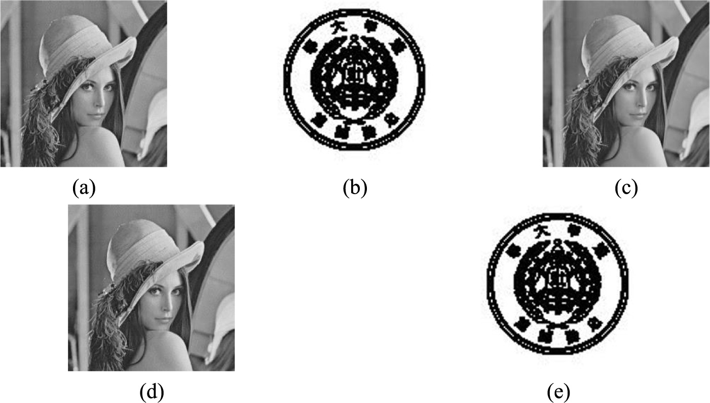
Figure 4: Results of an example experiment: (a) cover image; (b) secret image; (c) stego image (PSNR = 61.43 dB; payload = 10,000 bits); (d) recovered cover image; (e) extracted secret image

PSNR=10log10⁡(2552×W×H∑W×H(pi−pi′)2)(dB),(19)

where pi and pi′ represent the corresponding pixel values in the cover image and stego image, respectively. Theoretically, as long as the PSNR value is higher than 30 dB, it is difficult for humans to distinguish between the cover image and the stego image. The PSNR value of the stego image is 61.43 dB, which is much higher than 30 dB. This result can indicate that the stego image has high fidelity. Since the proposed scheme is reversible, the cover image and the secret data can be perfectly restored as shown in Figs. 4d and 4e.

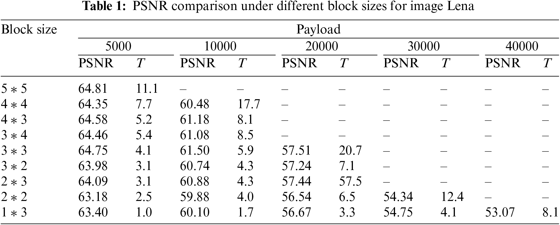
Fig. 5 and Table 1 show the performance comparison of the proposed scheme for different block sizes. It is worth mentioning that there are many other choices of block sizes, and only nine of them are taken as examples. As we can see, as the block size becomes smaller, the embedding capacity (EC) of the proposed scheme becomes larger, but the PSNR decreases sharply. Among them, the 5 * 5 size block has the best performance when the payload is 5000 bits, reaching 64.81. Since this size of the block is only suitable for smooth areas, it can only be used with a small payload. The 3 * 3 block performs best when the payload is increased to 10,000 and 20,000 bits, reaching 61.50 and 57.51, respectively. This result shows that the 3 * 3 block is more suitable for smooth and normal areas and can maintain good image quality even with moderate embedding capacity. When the embedding requirement increases, we can use smaller size blocks, such as 2 * 2, 1 * 3, etc., to sacrifice image quality for more embedding space.

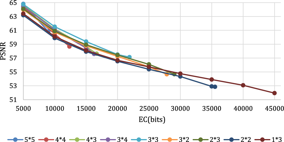
Figure 5: PSNR comparison under different block sizes for image Lena

4.2 Comparison with Other Schemes

Then, we compare the proposed scheme with nine state-of-the-art schemes of He et al. [11], Abolfazl et al. [12], Kong et al. [13], He et al. [14], He et al. [15], Yu et al. [16], Fan et al. [17], Zhang et al. [18], and Chang et al. [19]. Tables 2–4 show the comparison results of PSNR for embedding capacities with 5000 bits, 10,000 bits, and 20,000 bits. Also, the performance comparison between the proposed scheme and nine compared schemes is shown in Fig. 6. It noted that the block size and thresholds for different images are adaptively chosen. According to the tables and figures, it is easy to see that the proposed scheme has the best performance in most cases under moderate capacity.

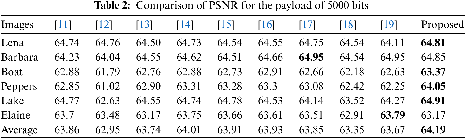
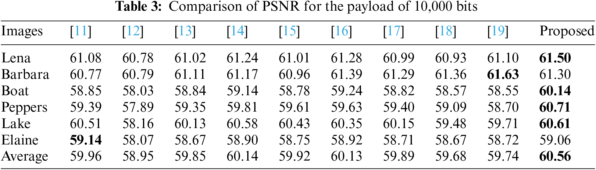
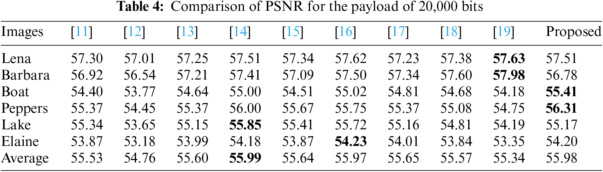
Figure 6: The performance comparison between the proposed scheme and nine compared schemes

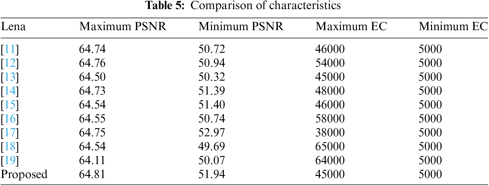
Based on the above experimental results, it is obvious that our schemes and the existing nine are quite competitive. To further explore the advantage of our proposed scheme, the relationship between the embedding capacity (EC) and corresponding image quality (PSNR) is summarized in Table 5 with the test image “Lena.” Here, we can see that our proposed scheme offers the highest image quality with 64.81 dB when secret bits are only 5000 bits. Although the largest hiding capacity of our proposed scheme is 45,000 bits, which is higher than in [17], the same as that of [13] and similar to those of [11] and [15] but less than those of the remaining schemes. Considering the largest hiding capacity among nine existing schemes and ours listed in Table 5, it can be found that schemes in [18] and [19] offer the largest hiding capacity, i.e., around 64,000∼65,000 bits. The computation complexity of the schemes in [18] and [19] and ours is O(K * b * m), O(K * b * m), and O(K * S), respectively, where K indicates the number of histograms, b indicates the number of pairs, m indicates the number of mappings, and S is the amount of bin for each histogram set. The computation complexity of our proposed scheme is relatively lower than the schemes in [18] and [19] and maintains a good balance between storage capacity and image quality. In other words, the proposed RDH scheme is suitable for real-time applications, i.e., IIoT or IoT, etc.

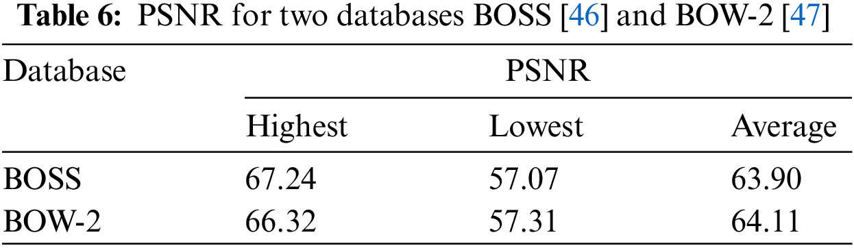
4.3 Applicability to Image Databases

In order to further evaluate the performance of the proposed scheme for various types of images, 100 images sized 512 × 512 are randomly selected from two databases (BOSS [46] and BOW-2 [47]) with a payload of 10,000 bits. As shown in Figs. 7a and 7b, the PSNR of selected images mainly ranges from 56 to 67 dB. Only three of the 200 test images have PSNR less than 58 dB. Therefore, our proposed scheme has universality and is applicable to most images. The indicators reflecting the trend of the data are shown in Fig. 7c. As illustrated in Fig. 8, it is obvious that the stego images with a high PSNR value are low-contrast images and vice versa. However, the superiority of the proposed scheme in terms of the image quality of the stego image can be demonstrated by the data in Table 6, including the maximum, minimum, and average values.

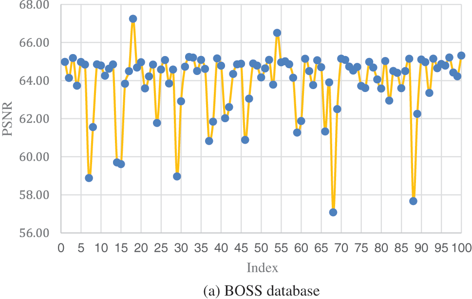
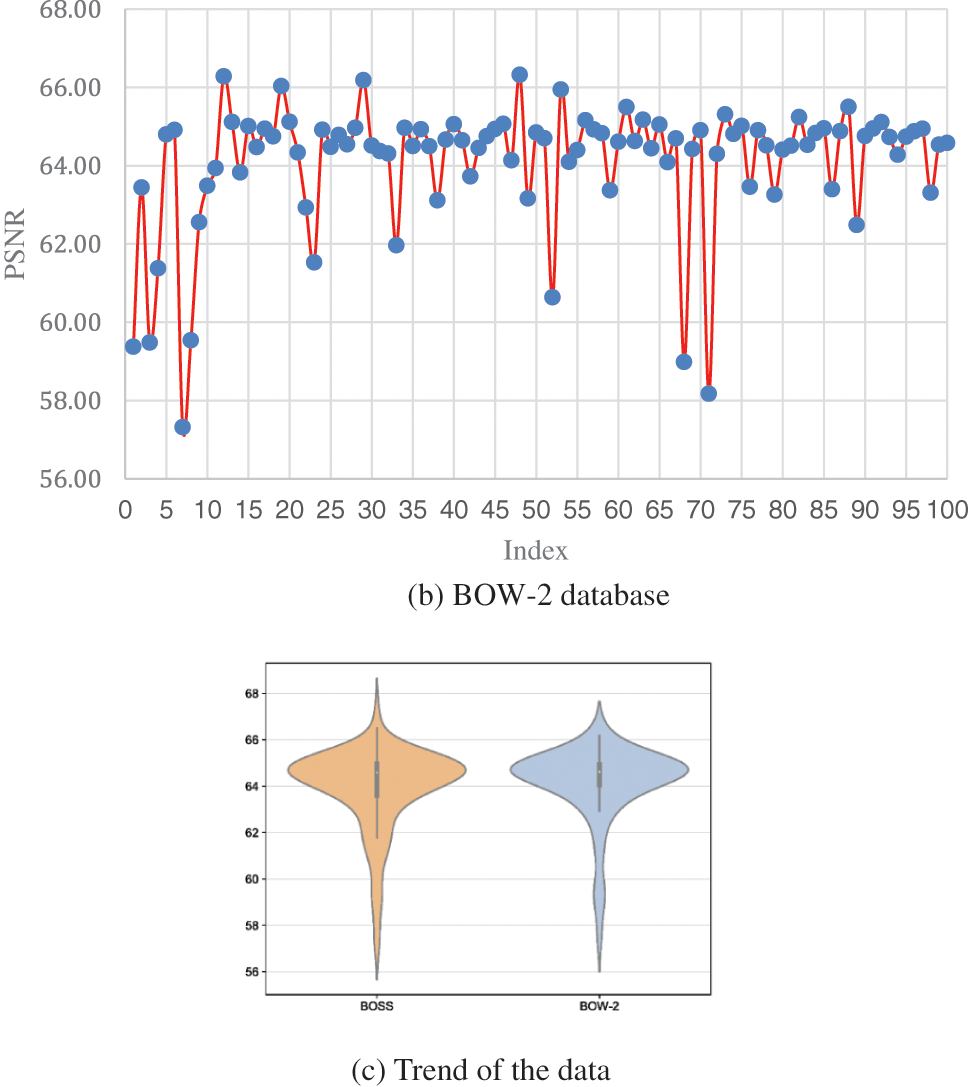
Figure 7: PSNR for 100 randomly selected images from BOSS [46] and BOW-2 [47]

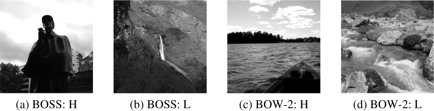
Figure 8: Images correspond to the highest and lowest PSNR values

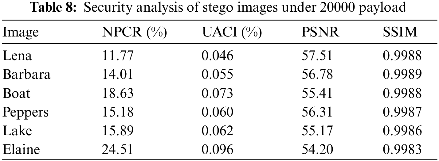
4.4 Security Analysis and Steganalysis

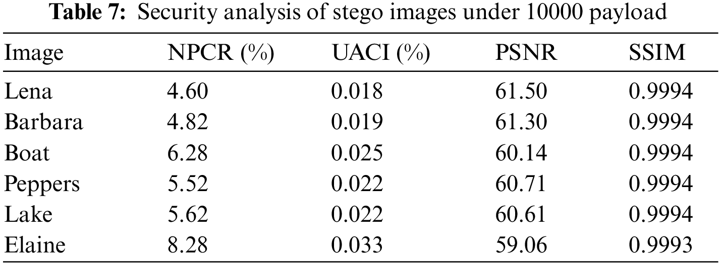
To estimate the security of the proposed scheme, we apply the number of pixels change rate (NPCR), the unified average changing intensity (UACI) and structural similarity (SSIM) to evaluate the performance of six stego images under 10000 and 20000 payloads. The definitions of NPCR, UACI and SSIM are

NPCR=∑i,jD(i,j)H×W×100%, where D(i,j)={1,O(i,j)≠S(i,j)0,otherwise,(20)

UACI=1H×W∑i,j|O(i,j)−S(i,j)|255×100%,(21)

SSIM(O,S)=(2μOμS+c1)(2σOS+c2)(μO2+μS2+c1)(σO2+σS2+c2),(22)

c1=(k1L)2, where k1=0.01,(23)

c1=(k2L)2, where k2=0.03,(24)

where μO and μS represent the average of O and S, respectively; σO2 and σS2 are the variances of O and S; σOS is the variance of O and S.

As shown in Tables 7 and 8, the NPCR and UACI values of the stego images are both low, indicating that the modification of the original image by the stego images is not easily detectable. The values of SSIM are very close to 1, representing that the stego image is very similar to the original image. The results of Tables 7 and 8 indicate that the stego image generated by the proposed scheme is not easily suspected by the attacker during transmission.

To verify whether the proposed scheme can guarantee the high-fidelity of the stego image, pixel value differencing (PVD) steganalysis [48] is used to test the stego images. The histograms of PVD are shown in Fig. 9. An analysis of two test images (“Lena” and “Boat”) is presented. To better compare the differences between the stego image and the cover image, we also draw the details of the histograms in the peak range. As shown in the figures, the histograms of embedded stego images under 10,000 and 20,000 bits are close to the histograms of the cover images. The analysis shows that the proposed scheme greatly preserves the characteristics of the cover image and achieves high-fidelity reversible data hiding.

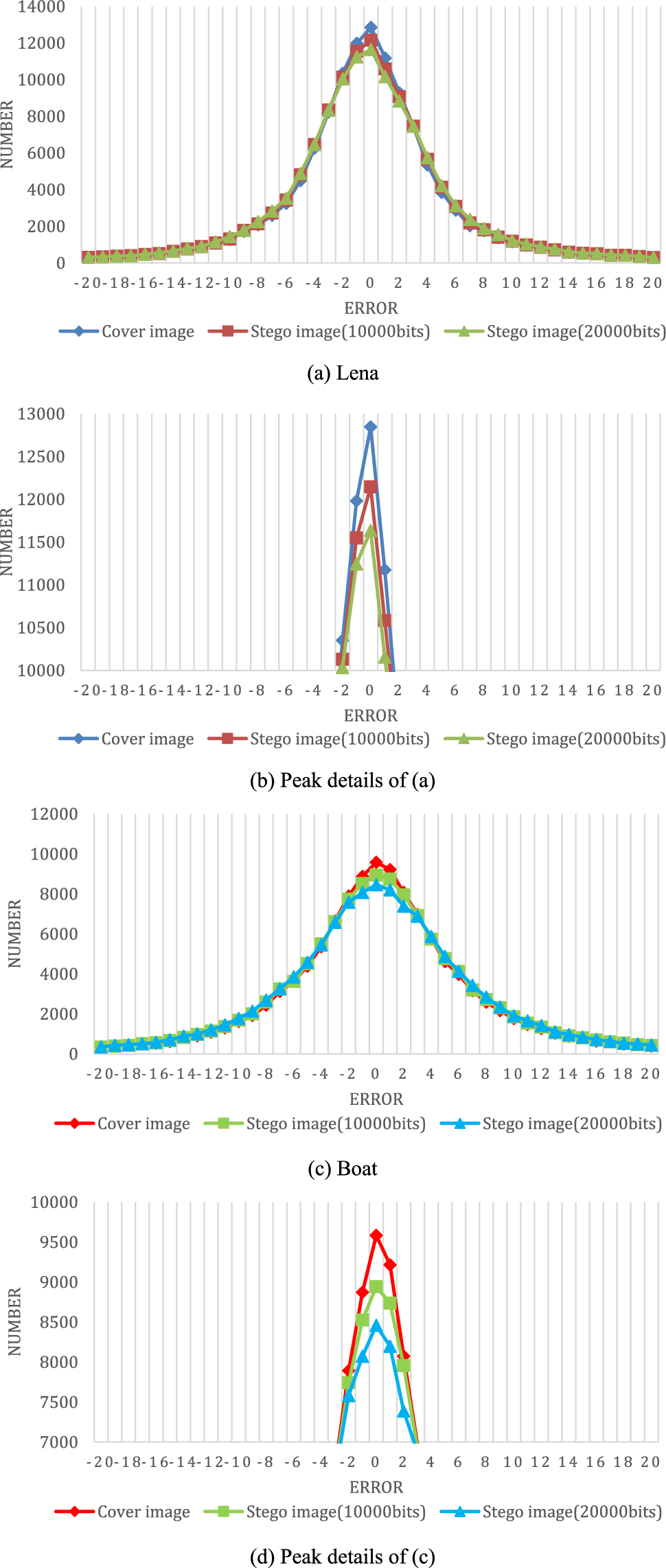
Figure 9: PVD analysis of the stego images and cover images

5  Conclusions

In this paper, a novel high-fidelity RDH scheme is proposed. Based on the multiprediction mechanism and multihistogram technique, the proposed scheme effectively improves the prediction accuracy as well as reduces the distortion of the cover image. Experimental results show that the quality of the stego image of our scheme outperforms the state-of-the-art schemes in most cases, especially for high-contrast cover images. In addition, we also confirm the high fidelity of the stego image by steganalysis. In the future, we will investigate how to further improve the quality of the stego image with more effective algorithms.

Acknowledgement: This paper is supported by Feng Chia University, Taichung, Taiwan and National of Chin-Yi University of Technology, Taichung, Taiwan.

Funding Statement: This paper is funded by National Science Council, Taiwan, the Grant Number is NSC 111-2410-H-167-005-MY2.

Author Contributions: The authors confirm the contribution to the paper as follows: Conceptualization: Kai Gao; Methodology: Kai Gao; Formal analysis and investigation: Chia-Chen Lin; Writing-original draft preparation: Kai Gao; Writing-review and editing: Chia-Chen Lin and Chin-Chen Chang; Resources: Chia-Chen Lin and Chin-Chen Chang; Supervision: Chin-Chen Chang.

Availability of Data and Materials: Not applicable.

Conflicts of Interest: The authors declare that they have no conflicts of interest to report regarding the present study.

References

1. H. Jiang et al., “FAWA: Fast adversarial watermark attack,” IEEE Trans. Comput., vol. 73, no. 2, pp. 301–313, 2024. [Google Scholar]

2. C. P. Wang et al., “CWAN: Covert watermarking attack network,” Electronics, vol. 12, no. 2, pp. 1–12, 2023. [Google Scholar]

3. M. Kaur, S. Singh, and M. Kaur, “Computational image encryption techniques: A comprehensive review,” Math. Probl. Eng., vol. 2021, pp. 1–17, 2021. [Google Scholar]

4. G. Kulkarni et al., “BabyTalk: Understanding and generating simple image descriptions,” IEEE Trans. Pattern Anal. Mach. Intell., vol. 35, no. 12, pp. 2891–2903, 2013 [Google Scholar] [PubMed]

5. P. Kinghorn, L. Zhang, and L. Shao, “A region-based image caption generator with refined descriptions,” Neurocomputing, vol. 272, pp. 416–424, 2018. [Google Scholar]

6. Y. J. Xian and X. Y. Wang, “Fractal sorting matrix and its application on chaotic image encryption,” Inf. Sci., vol. 547, no. 8, pp. 1154–1169, 2021. [Google Scholar]

7. Z. C. Ni, Y. Q. Shi, N. Ansari, and W. Su, “Reversible data hiding,” IEEE Trans. Circuits Syst. Video Technol., vol. 16, no. 3, pp. 345–362, 2006. [Google Scholar]

8. S. Kumar, A. Gupta, and G. S. Walia, “Reversible data hiding: A contemporary survey of state-of-the-art, opportunities and challenges,” Appl. Intell., vol. 52, pp. 7373–7406, 2022. [Google Scholar]

9. C. C. Chang, C. T. Li, and K. M. Chen, “Privacy-preserving reversible information hiding based on arithmetic of quadratic residues,” IEEE Access, vol. 7, pp. 54117–54132, 2019. [Google Scholar]

10. Y. Q. Chen, W. J. Sun, L. Y. Li, C. C. Chang, and X. Wang, “An efficient general data hiding scheme based on image interpolation,” J. Inf. Secur. Appl., vol. 54, pp. 102854, 2020. [Google Scholar]

11. W. G. He and Z. C. Cai, “An insight into pixel value ordering prediction-based prediction-error expansion,” IEEE Trans. Inf. Forensics Secur., vol. 15, pp. 3859–3871, 2020. [Google Scholar]

12. K. Abolfazl and M. H. Sedaaghi, “Reversible data hiding based on high fidelity prediction scheme for reducing the number of invalid modifications,” Inf. Sci., vol. 589, pp. 46–61, 2022. [Google Scholar]

13. X. X. Kong and Z. C. Cai, “An information security method based on optimized high-fidelity reversible data hiding,” IEEE Trans. Ind. Inform., vol. 18, no. 22, pp. 8529–8539, 2022. [Google Scholar]

14. W. G. He and Z. C. Cai, “Reversible data hiding based on dual pairwise prediction-error expansion,” IEEE Trans. Image Process., vol. 30, pp. 5045–5055, 2021 [Google Scholar] [PubMed]

15. W. G. He, Z. C. Cai, and Y. M. Wang, “High-fidelity reversible image watermarking based on effective prediction error-pairs modification,” IEEE Trans. Multimed., vol. 23, pp. 52–63, 2020. [Google Scholar]

16. C. Q. Yu, X. Q. Zhang, D. W. Wang, and Z. J. Tang, “Reversible data hiding with pairwise PEE and 2D-PEH decomposition,” Signal Process., vol. 196, pp. 108527, 2022. [Google Scholar]

17. G. J. Fan, Z. B. Pan, E. D. Gao, X. Y. Gao, and X. R. Zhang, “Reversible data hiding method based on combining IPVO with bias-added rhombus predictor by multi-predictor mechanism,” Signal Process., vol. 180, pp. 107888, 2021. [Google Scholar]

18. C. Zhang and B. Ou, “Reversible data hiding based on multiple adaptive two-dimensional prediction-error histograms modification,” IEEE Trans. Circuits Syst. Video Technol., vol. 32, no. 7, pp. 4174–4187, 2021. [Google Scholar]

19. Q. Chang, X. L. Li, Y. Zhao, and R. R. Ni, “Adaptive pairwise prediction-error expansion and multiple histograms modification for reversible data hiding,” IEEE Trans. Circuits Syst. Video Technol., vol. 31, no. 12, pp. 4850–4863, 2021. [Google Scholar]

20. A. Malik, H. X. Wang, Y. L. Chen, and A. N. Khan, “A reversible data hiding in encrypted image based on prediction-error estimation and location map,” Multimed. Tools Appl., vol. 79, pp. 11591–11614, 2020. [Google Scholar]

21. X. C. Cao, L. Du, X. X. Wei, D. Meng, and X. J. Guo, “High capacity reversible data hiding in encrypted images by patch-level sparse representation,” IEEE Trans. Cybern., vol. 46, no. 5, pp. 1132–1143, 2015 [Google Scholar] [PubMed]

22. B. Chen, W. Lu, J. W. Huang, J. Weng, and Y. C. Zhou, “Secret sharing based reversible data hiding in encrypted images with multiple data-hiders,” IEEE Trans. Dependable Secure Comput., vol. 19, no. 2, pp. 978–991, 2015. [Google Scholar]

23. C. H. Yang, C. Y. Weng, and Y. J. Chen, “High-fidelity reversible data hiding in encrypted image based on difference-preserving encryption,” Soft Comput., vol. 26, pp. 1727–1742, 2022. [Google Scholar]

24. F. Huang, J. Huang, and Y. Q. Shi, “New framework for reversible data hiding in encrypted domain,” IEEE Trans. Inf. Forensics Secur., vol. 11, no. 12, pp. 2777–2789, 2016. [Google Scholar]

25. F. Li, Q. Mao, and C. C. Chang, “A reversible data hiding scheme based on IWT and the sudoku method,” Int. J. Netw. Secur., vol. 18, pp. 410–419, 2014. [Google Scholar]

26. H. Zhang and L. T. Hu, “A data hiding scheme based on multidirectional line encoding and integer wavelet transform,” Signal Process. Image Commun., vol. 78, pp. 331–334, 2019. [Google Scholar]

27. C. Y. Yang and W. C. Hu, “Reversible data hiding in the spatial and frequency domains,” Int. J. Image Process., vol. 3, no. 6, pp. 373–384, 2010. [Google Scholar]

28. M. Y. Xiao, X. L. Li, and Y. Zhao, “Reversible data hiding for JPEG images based on multiple two-dimensional histograms,” IEEE Signal Process. Lett., vol. 28, pp. 1620–1624, 2021. [Google Scholar]

29. Z. Qian, X. Zhang, and S. Wang, “Reversible data hiding in encrypted JPEG bitstream,” IEEE Trans. Multimed., vol. 16, no. 5, pp. 1486–1491, 2014. [Google Scholar]

30. J. Tian, “Reversible data embedding using a difference expansion,” IEEE Trans. Circuits Syst. Video Technol., vol. 13, no. 8, pp. 890–896, 2003. [Google Scholar]

31. Y. J. Hu, H. K. Lee, K. Y. Chen, and J. W. Li, “Difference expansion based reversible data hiding using two embedding directions,” IEEE Trans. Multimed., vol. 10, no. 8, pp. 1500–1512, 2008. [Google Scholar]

32. D. M. Thodi and J. J. Rodriguez, “Expansion embedding techniques for reversible watermarking,” IEEE Trans. Image Process., vol. 16, no. 3, pp. 721–730, 2007 [Google Scholar] [PubMed]

33. R. Kumar, D. Sharma, A. Dua, and K. H. Jung, “A review of different prediction methods for reversible data hiding,” J. Inf. Secur. Appl., vol. 78, pp. 103572, 2023. [Google Scholar]

34. L. Luo, Z. Chen, M. Chen, X. Zeng, and Z. Xiong, “Reversible image watermarking using interpolation technique,” IEEE Trans. Inf. Forensics Secur., vol. 5, no. 1, pp. 187–193, 2009. [Google Scholar]

35. I. C. Dragoi and D. Coltuc, “Local-prediction-based difference expansion reversible watermarking,” IEEE Trans. Image Process., vol. 23, no. 4, pp. 1779–1790, 2014 [Google Scholar] [PubMed]

36. R. W. Hu and S. J. Xiang, “CNN prediction based reversible data hiding,” IEEE Signal Process. Lett., vol. 28, pp. 464–468, 2021. [Google Scholar]

37. X. L. Li, W. M. Zhang, X. L. Gui, and B. Yang, “Efficient reversible data hiding based on multiple histograms modification,” IEEE Trans. Inf. Forensics Secur., vol. 10, no. 9, pp. 2016–2027, 2015. [Google Scholar]

38. V. Sachnev, H. J. Kim, J. Nam, S. Suresh, and Y. Q. Shi, “Reversible watermarking algorithm using sorting and prediction,” IEEE Trans. Circuits Syst. Video Technol., vol. 19, no. 7, pp. 989–999, 2009. [Google Scholar]

39. X. L. Li, J. Li, B. Li, and B. Yang, “High-fidelity reversible data hiding scheme based on pixel-value-ordering and prediction-error expansion,” Signal Process., vol. 93, pp. 198–205, 2013. [Google Scholar]

40. O. Bo, X. L. Li, Y. Zhao, and R. R. Ni, “Reversible data hiding using invariant pixel-value-ordering and prediction-error expansion,” Signal Process., vol. 29, pp. 760–772, 2014. [Google Scholar]

41. F. Peng, X. L. Li, and B. Yang, “Improved PVO-based reversible data hiding,” Digit. Signal Process., vol. 25, pp. 255–265, 2014. [Google Scholar]

42. X. Wang, L. Ding, and Q. Q. Pei, “A novel reversible image data hiding scheme based on pixel value ordering and dynamic pixel block partition,” Inf. Sci., vol. 310, pp. 16–35, 2015. [Google Scholar]

43. X. C. Qu and H. J. Kim, “Pixel-based pixel value ordering predictor for high-fidelity reversible data hiding,” Signal Process., vol. 111, pp. 249–260, 2015. [Google Scholar]

44. X. Ma, Z. Pan, S. Hu, and L. Wang, “High-fidelity reversible data hiding scheme based on multi-predictor sorting and selecting mechanism,” J. Vis. Commun. Image Represent., vol. 28, pp. 71–82, 2015. [Google Scholar]

45. M. J. Weinberger, G. Seroussi, and G. Sapiro, “The LOCO-I lossless image compression algorithm: Principles and standardization into JPEG-LS,” IEEE Trans. Image Process., vol. 9, no. 8, pp. 1309–1324, 2000 [Google Scholar] [PubMed]

46. P. Bas, T. Filler, and T. Pevný, “Break our steganographic system—the ins and outs of organizing BOSS,” in Int. Workshop Inform. Hiding, Berlin, Heidelberg, Springer, 2011, pp. 59–70. [Google Scholar]

47. A. Gupta, “BOWS2,” 2017. Mendeley Data, Vl. NCU, 2023. doi: 10.17632/kb3ngxfmjw.l. [Google Scholar] [CrossRef]

48. X. Zhang and S. Wang, “Vulnerability of pixel-value differencing steganography to histogram analysis and modification for enhanced security,” Pattern Recognit. Lett., vol. 25, no. 3, pp. 331–339, 2004. [Google Scholar]