Fuzzy C-Means Algorithm Based on Density Canopy and Manifold Learning

1  Introduction

Clustering is an unsupervised learning process that divides an unlabeled dataset into a number of un-known labeled clusters [1]. Clustering algorithms are commonly used in many fields such as e-commerce, image segmentation, medical diagnosis, and emotion analysis [2–6]. Clustering algorithms are classified into five types based on different learning strategies such as division, constraint, hierarchy, density, and grid. Fuzzy C-Means algorithms belong to the division-based clustering type, which utilizes membership to determine the degree of subordination of each data object to a certain class cluster [7]. The Fuzzy C-Means algorithm has been commonly used because of its simplicity and flexibility and efficient clustering. However, the traditional FCM algorithm is sensitive to the initial cluster center. Furthermore, Euclidean distance is only suitable for global linear structure data, and complex high-dimensional data often present nonlinear structure.

Many improvement algorithms have been proposed to address the shortcomings of Fuzzy C-Means. Several researchers [8–10] improved the Fuzzy C-Means algorithm using the meta-heuristic algorithm to overcome the high dependence on initial cluster centers. Liu et al. [11] combined the density peaking algorithm with the Fuzzy C-Means algorithm to improve the convergence ability and clustering accuracy of the Fuzzy C-Means algorithm. Bei et al. [12] combined the grey correlation and weighted distance method to improve the accuracy of clustering results. Chen et al. [13] presented a weight parameter-based method to improve the Fuzzy C-Means of likelihood fuzziness, which has good performance in processing noisy data. Liu et al. [14] introduced feature reduction and incremental strategies to process large-scale data clustering. Cardone et al. [15] proposed the Shannon fuzzy entropy function to assign weights to attain clustering centers, which improves the clustering performance of the FCM algorithm. The combination of Minkowski distance and Chebyshev distance is introduced as a similarity measure for the FCM algorithm to improve the clustering accuracy by Surono et al. [16]. Zhang et al. [17] combined do-main information constraints and deviated sparse Fuzzy C-Means to obtain clustering centers, which im-proved the clustering efficiency. Tang et al. [18] combined a novel membership model based on rough sets [19,20] and an inhibitive factor with the FCM algorithm, which improved the convergence speed and reduced the influence of cluster edge noise data. Gao et al. [21] proposed a Gaussian mixture model and collaborative technique to solve the clustering problem of non-spherical data sets in the Fuzzy C-Means algorithm. In addition, fuzzy clustering algorithms are used in a wide range of real-world applications. Deveci et al. [22] proposed a hybrid model based on q-rung orthopair fuzzy sets (q-ROFSs) which is applied as a guide for decision-makers of the metaverse when integrating autonomous vehicles into the transportation system. Alharbi et al. [23] proposed a hybrid approach based on dictionaries and fuzzy inference process (FIP), which uses a fuzzy system to identify textual sentiment while solving the problem of sentiment analysis. Alsmirat et al. [24] applied the Fuzzy C-Means to the image seg-mentation algorithm, which uses the graphics processing unit (GPU) function to speed up the execution time of the algorithm.

The above methods have limitations because the actual data sets often present complex high-dimensional nonlinear structures. In addition, the number of clusters and random cluster center selection has a significant impact on the clustering accuracy of the FCM algorithm. Therefore, more representative initial cluster centers are required to select. Fusing the local dissimilarity of the dataset with the global dissimilarity gives better feedback for the original distribution of the dataset. In this paper, the density Canopy algorithm is applied to the Fuzzy C-Means algorithm for the first time and improves the calculation of local density. The improved density Canopy algorithm automatically selects the appropriate initial cluster centers, automatically determines the number of clusters, and improves the adaptability and stability of the FCM algorithm. In addition, this paper also uses the manifold learning method as a dissimilarity measure for the clustering process. It can better focus on the global geometric properties of nonlinear data and thus address the inefficiency of clustering practical complex high-dimensional data.

For this paper, the main contributions are as follows:

(1)   We optimize the objective function of the FCM algorithm by means of a distance metric based on manifold learning. This nonlinear dimensionality reduction algorithm calculates the global optimal solution and preserves the true structure of the data, thus improving the clustering accuracy under complex high-dimensional data.

(2)   We have improved the density Canopy algorithm so as to better adapt to data with different density distributions. The improved density Canopy algorithm automatically determines the number of clusters and picks the appropriate initial cluster centers, which improves the adaptiveness and stability of the FCM clustering algorithm.

(3)   We validate the comprehensive effectiveness of the DM-FCM algorithm on various datasets (7 artificial datasets and 7 UCI datasets), demonstrate that the manifold learning method is a superior distance metric, and verify higher effectiveness in clustering complex high-dimensional data.

2  Fuzzy C–Means Algorithm

2.1 Principle of Fuzzy C-Means Algorithm

Given a dataset X={x1,x2,…,xn}, the Fuzzy C-Means algorithm utilizes the membership degree uij to represent the probability of the data object xj belonging to cluster ci, assigns xj to the corresponding cluster with the largest membership degree, and iteratively calculates to finally obtain k clusters. The objective function of the Fuzzy C-Means algorithm is shown in Eq. (1), where m is the fuzzy constant (generally m = 2), and ∥xj−ci∥ represents the distance between data object xj and the cluster center ci.

J=∑i=1k∑j=1nuijm∥xj−ci∥2(1)

The detailed steps of the Fuzzy C-Means algorithm are as follows:

Step 1: Determine the number of clusters k, and then determine initial cluster centers.

Step 2: Compute the membership degree according to Eq. (2)

uij=1∑k=1c(xj−cixj−ck)2m−1(2)

Step 3: Compute the cluster center according to Eq. (3)

ci=∑j=1nuijm∑j=1nuijmxj(3)

Step 4: If ∥J(t)−J(t+1)∥>ε, return to Step 2 for repetition; otherwise, the algorithm ends.

2.2 Problems with Fuzzy C-Means Algorithm

The Fuzzy C-Means algorithm manually selects the number of clusters as the input parameter affecting its adaptiveness. In addition, the randomly selected initial cluster centers affect the stability of the algorithm. The Fuzzy C-Means algorithm utilizes the Euclidean distance as a distance measure, but the high-dimensional space often presents a nonlinear structure, and it is difficult to calculate the global consistency of the dataset by directly calculating the linear distance. To address the above problems, the FCM clustering algorithm that integrates manifold learning and density Canopy based on improved local density is proposed, using the density Canopy algorithm for pre-clustering, which automatically finds the appropriate initial cluster centers without the tedious step of manually selecting cluster centers. Meanwhile, manifold learning is used as the distance measure, and this global nonlinear manifold learning method preserves the global consistency of the high-dimensional nonlinear space and improves the clustering accuracy of high-dimensional data.

3  Density Canopy Algorithm

3.1 Related Concepts

Given a dataset D={x1,x2,…,xn}, the data object xi in D is noted as xi={xi1,xi2,…,xid}. where xit represents the tth dimensional feature of the ith data object, and dij is the distance between the data objects xi and xj.

Definition 1 MeanD(D) is the average distance of all data objects in dataset D:

MeanD(D)=2n(n−1)∑i=1n∑j=i+1ndij(4)

Definition 2 The distance between other data objects and data object xi is less than MeanD(D), thus forming a cluster, and the number of data objects in the cluster is local density ρi:

ρi=∑j=1nf[dij−MeanD(D)](5)

where f(x)={1,x<00,x≥0

Definition 3 The average distance of all data objects in the cluster:

ai=2ρi(ρi−1)∑i=1ρi∑j=i+1ρidij(6)

Definition 4 If there are other data objects xj with a larger density value than the data object xi, The inter-cluster distance si is the minimum value in the distance set of the data objects xj with larger local density values. If the local density value of data object xi is the maximum value in the dataset, then The inter-cluster distance si is the maximum value in the set of dissimilarities of data object xj with smaller local density values.

si={min(dij)xj:ρj>ρi,∃j,ρj>ρimax(dij)xj∈D,∀j,ρj<ρi(7)

Definition 5 The weight ωi of the cluster center of the data object, where the density value ρi indicates the compactness degree between data objects in the cluster where this data object is located. The smaller the value ai is, the more compact the data object in this cluster is and the smaller the distance the data object in this cluster is. si indicates the distance between this data object and other clusters.

ωi=ρi∗1ai∗si(8)

3.2 Algorithm Flow

The Density Canopy algorithm selects the data with the highest density value as the first cluster center and removes data with a distance less than MeanDist(D) from this cluster center. Then the data with the highest cluster center weight is selected as the next cluster center, and the data with a distance less than MeanDist(D) from this cluster center is removed. Iterate until the data set is empty to attain the set of cluster centers. The density Canopy algorithm solves the problem that the Canopy algorithm needs to manually input the parameter thresholds in advance and the parameter thresholds are difficult to determine. It adaptively calculates the truncation distance threshold and improves the adaptability and stability of the Canopy algorithm.

Density Canopy Algorithm

Input: Dataset D

Output: Initial cluster center C(0)

Step 1: Use Eq. (4) to obtain MeanDist(D), use Eq. (5) to obtain the density ρi of each data, obtain the first cluster center by selecting the data with the highest density in the dataset, and add the cluster center c1 to the cluster center set, so C(0)={c1}. Then delete the remaining data objects with a distance less than MeanDist(D) to the first cluster center.

Step 2: According to the Eqs. (5)–(7), the ρi, ai, and si of the remaining data objects are calculated, and then the cluster center weights ωi are obtained from the Eq. (8), and the next cluster center c2 is obtained by selecting the data with the largest cluster center weight value, and adding it to the set of cluster centers C(0)={c1,c2}. The data objects with a distance less than MeanDist(D) among the remaining data objects in the data set are deleted.

Step 3: Repeat step 2 until dataset D is empty.

Step 4: Redetermine the cluster center of each cluster. Iterate through the data objects of each cluster, calculate the distance between the data object and other data objects in this cluster, and obtain the cluster center of this cluster by selecting the data with the smallest sum of distance in this cluster Ci(0).

4  FCM Algorithm Based on Density Canopy and Manifold Learning

4.1 Distance Measurement Based on Manifold Learning Principle

The distance measure of the Fuzzy C-Means algorithm is based on the Euclidean distance, but as the data dimension of the dataset grows, it is difficult to calculate the linear distance in the high-dimensional space to measure the global consistency of the dataset. The basic principle of the manifold learning algorithm is to introduce the K-nearest neighbor idea to calculate the geodesic distance between each data object. For nearest neighbor data objects, Euclidean distance is used as their geodesic distance. For non-nearest neighbor data objects, the nearest neighbor graph is constructed and the shortest path algorithm is used to calculate the shortest path between data objects as the geodesic distance, and multidimensional scaling (MDS) is used to reduce the dimensionality to obtain the dissimilarity matrix in the low-dimensional space. The manifold learning method is a global nonlinear dimensionality reduction algorithm, which approximates the geometric structure of data objects in high-dimensional space by constructing a nearest neighbor graph, preserving the global geometric properties of high-dimensional manifold data.

Manifold learning algorithm flow is as follows:

Input: dataset X={x1,x2,…,xn∈RN}, number of neighbors K, reduced dimension d

Output: low-dimensional embedding coordinates Y={y1,y2,…,yn∈Rd}

Step 1: Construct the K-nearest neighbor graph G

Since the manifold is locally homogeneous with the Euclidean space, a nearest-neighbor connectivity graph is constructed for each data object by finding its nearest-neighbor points, in which there are connections between nearest-neighbor objects but not between non-neighbor objects. Then, the nearest neighbor connection graph is used to compute the shortest path between any two data objects, which approximates the geodesic distance on the low-dimensional embedded manifold. The K-nearest neighbor method is used to connect each data object with its k nearest data objects, construct a weighted K-nearest neighbor graph G, and calculate the path weights between the nearest K data objects, the path weight of each edge in the K-nearest neighbor graph G is dE(i,j), dE(i,j) represents the Euclidean distance between data object xi and data object xj.

Step 2: Compute the shortest path (Dijkstra’s algorithm)

Calculate the geodesic distance of any two data objects in the high-dimensional space. If data objects xi and xj are connected in graph G, the initial value of the shortest path between them is dG(i,j)=dE(i,j), otherwise it is dG(i,j)=∞. Let q = 1,2,...,N, where N is the total number of data objects, and the calculation method of the geodesic distance is shown in Eq. (9).

dG(i,j)=min{dG(i,j),dG(i,q)+dG(q,j)}(9)

Step 3: Calculate the low-dimensional embedding coordinates

The basic idea of multidimensional scaling is to map the distances between data objects from multidimensional space to low-dimensional space by matrix transformation, and to obtain low-dimensional coordinates that maintain the global geometric properties of the internal manifold by minimizing the objective function Eq. (10).

where DY denotes the distance matrix {dY(i,j)=||yi−yj||} of the low-dimensional embedded coordinates, ||A||L2=∑ijAij2 is the L2 matrix parametrization, the matrix operation operator τ(D)=−HSH/2, S is the matrix {Sij=Dij2} composed of distance squares, and H represents the centralized matrix {Hij=δij−1/N}. λp is the pth eigenvalue of τ(DG) and vp is the corresponding eigenvector of λp. When Y is the eigenvector corresponding to the d largest eigenvalues of M, then N and Eq. (10) reaches the global minimum.

E=‖τ(DG)−τ(DY)‖L2(10)

4.2 Density Canopy Algorithm Based on the Improved Local Density

The density Canopy algorithm ignores the nonlinear space and inhomogeneous density distribution among the actual data objects. In order to improve the adaptability of the density Canopy algorithm to different density distributions, the density Canopy algorithm based on the improved local density is proposed. The improved local density method first calculates the average manifold distance as the neighborhood distance, then calculates the number of data objects that are within the neighborhood distance from the data objects, and finally calculates the sum of the distance of data objects within the neighborhood distance. The relationship between the number of data objects and the sum of distances within the fused neighborhood distance results in a high similarity between data objects in the high-density distribution and a low similarity between data objects in the low-density distribution, thus improving the differentiation between clusters. The local density of the density Canopy algorithm is defined as:

ρi=∑j=1n[Rijf[Rij−MeanD(D)]]∑j=1nf[Rij−MeanD(D)](11)

where Rij is the manifold distance between data objects xi and xj, and MeanD(D) is the average manifold distance.

4.3 FCM Algorithm Fusing Manifold Learning and Density Canopy

To address the problem that the Fuzzy C-Mean algorithm needs to manually determine the number of clusters and randomly select the initial cluster centers in advance, the improved algorithm DM-FCM uses the density Canopy algorithm to automatically determine the number of clusters and initial cluster centers to improve the stability and self-adaptability of the FCM algorithm. To address the problem that the Euclidean distance metric in high-dimensional space cannot take into account the global consistency of data, the improved algorithm DM-FCM uses the manifold learning method as the distance metric of the FCM algorithm. The global consistency of high-dimensional data objects is preserved, thus improving the clustering quality of the FCM algorithm.

DM-FCM algorithm:

Input:

Dataset D;

number of neighbors K;

Convergence threshold: ε;

Output:

Clustering results of DM-FCM

Step 1: Determine the initial cluster center

Step 1.1 Use Eq. (11) to calculate the density ρi. Select the data with the largest density in the data set to get the first cluster center c1, while adding to the set of cluster centers C(0)={c1}, and then delete the data objects in the cluster.

Step 1.2 Update ρi, calculate ai by Eq. (6), calculate si by Eq. (7).and then use Eq. (8) to calculate the cluster center weights ωi. The data object with the largest cluster center weight value is selected as the next cluster center ci and added to the cluster center set C(0) at the same time, and the data objects within the cluster are then deleted.

Step 1.3 Repeat step 1.2 until the dataset D is empty.

Step 1.4 Redetermine the cluster centers of each cluster. The data object with the smallest sum of manifold distances in each cluster is selected as the cluster center Ci(0).

Step 2: Execute the FCM algorithm

Step 2.1 Initialize the iteration number t = 0.

Step 2.2 The dissimilarity matrix is updated using the manifold learning method, while the membership matrix uij(t) is calculated according to Eq. (2).

Step 2.3 Calculate the objective function value J(t) according to Eq. (1).

Step 2.4 Update the set of cluster centers C(t+1) according to Eq. (3).

Step 2.5 Update the membership matrix uij(t+1) according to Eq. (2).

Step 2.6 Compute the objective function value J(t+1) according to Eq. (1).

Step 2.7If ∥J(t)−J(t+1)∥<ε, exit; otherwise t=t+1, return to step 2.4.

The algorithm flow is shown in Fig. 1.

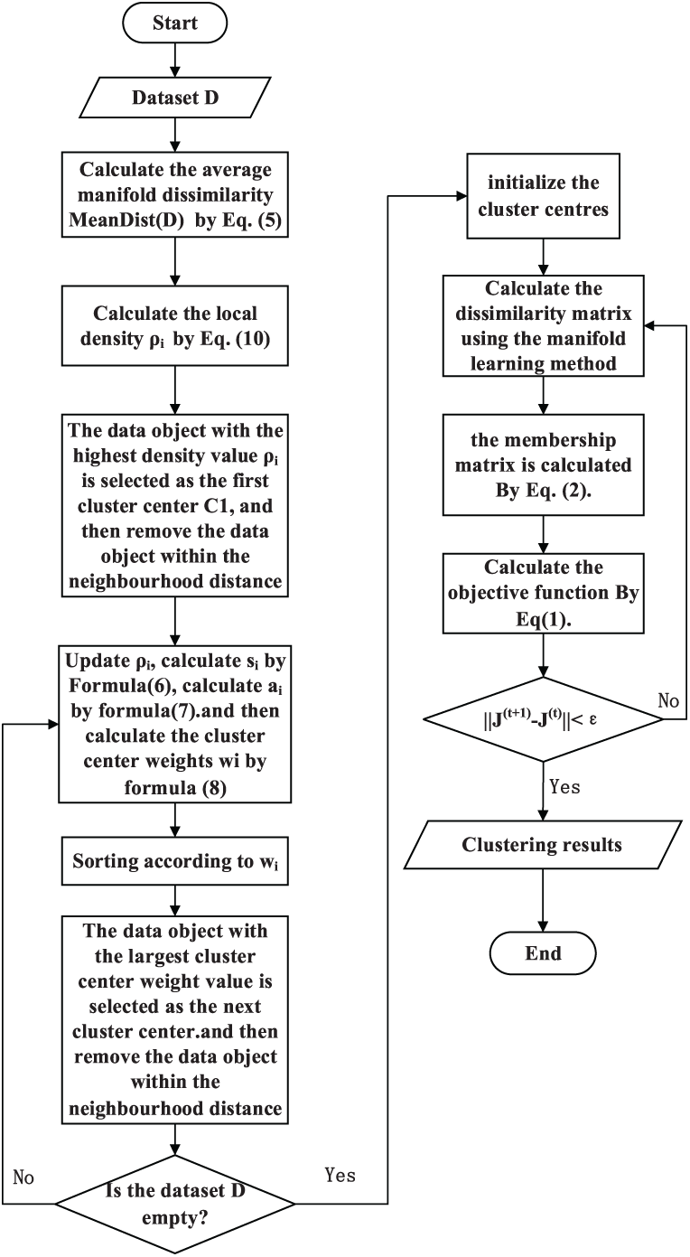
Figure 1: DC-IFCM algorithm flow chart

4.4 Algorithm Time Complexity Analysis

The time complexity of this algorithm comes primarily from the time complexity of the density Canopy algorithm and the FCM algorithm. Iterating over each data object, the time complexity of computing the manifold neighborhood distance is O(n2log⁡n), and then the time complexity of calculating the cluster center weights is O(n). So the time complexity of the density Canopy algorithm is O(n(n2log⁡n+n)). In addition, the time complexity of the FCM algorithm based on the manifold learning method is O(n2log⁡n+ndc2t), where d is the data dimensions, c is the number of clusters, and t is the number of iterations. Therefore, the total time complexity of the algorithm is O(n3log⁡n+ndc2t).

5  Simulation Results

Experimental environment: The algorithm experiment uses Windows10 operating system, Intel (R) Xeon(R) CPU E3-1225 v6 @ 3.30 GHz, 32 G memory, and Pycharm2019 simulation software.

5.1 Experimental Data

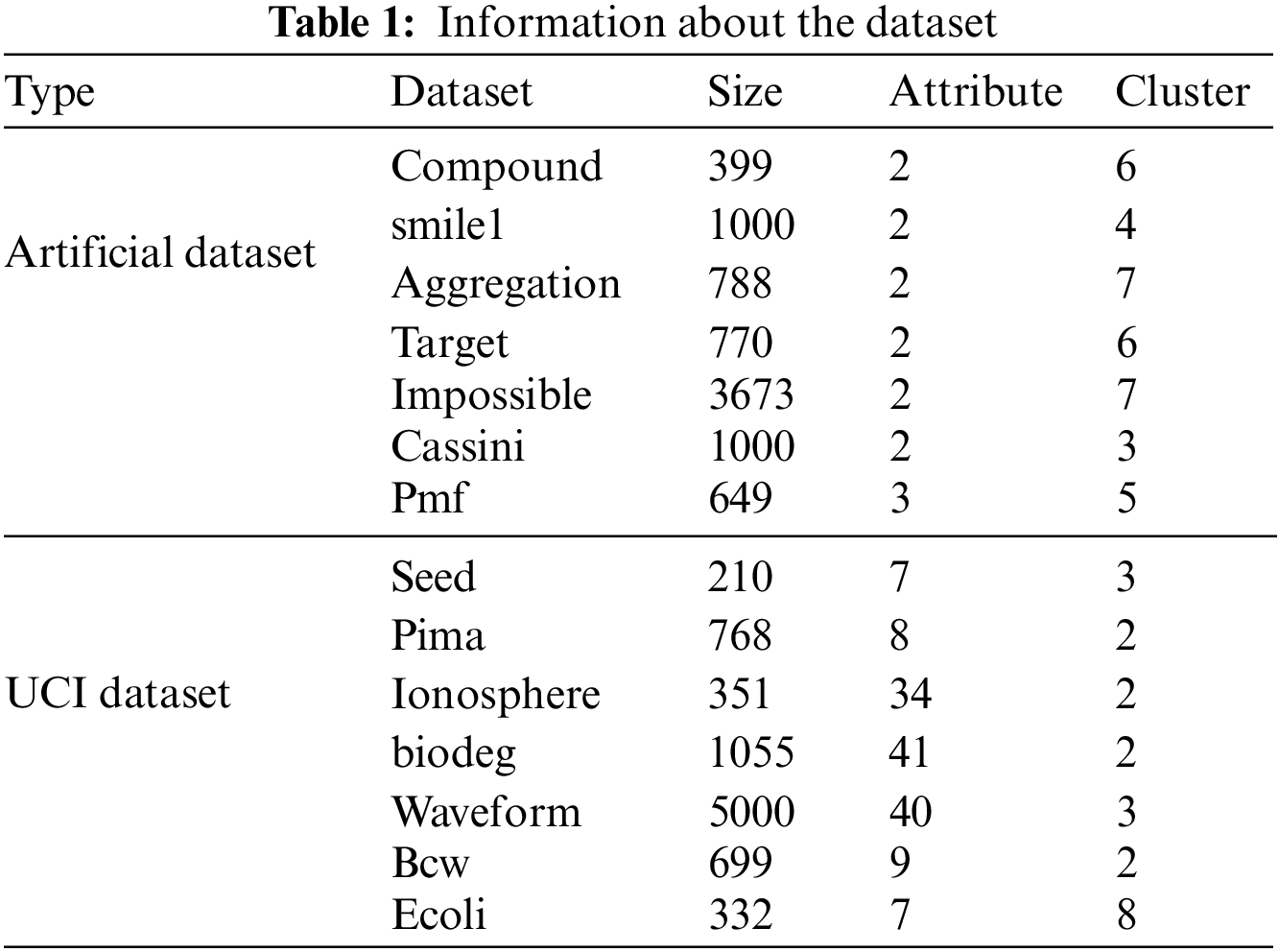
To verify the effectiveness of the DM-FCM algorithm, the experiment compares the DM-FCM algorithm with the FCM algorithm, Canopy-FCM algorithm, Single Pass Fuzzy C Means (SPFCM) algorithm, clustering by fast search and finding of density peaks (CFSFDP) algorithm and Weight Possibilistic Fuzzy C-Means Clustering Algorithm (WPFCM). Seven artificial datasets and seven high-dimensional UCI datasets were used for the experiments, and the information of the datasets is shown in Table 1.

5.2 Clustering Evaluation Indexes

To evaluate the clustering performance, FMI, V-measure, AMI (Adjusted Mutual Information), and ARI are used as the performance measures of the clustering algorithm.

The FMI is defined as follows, the larger the FMI, the higher the clustering validity, where TP denotes the number of sample pairs that belong to the same cluster in both true label and clustering results, FP denotes the number of sample pairs that belong to the same cluster in true label and do not belong to the same cluster in clustering results, and FN denotes the number of sample pairs that do not belong to the same cluster in true labels and belong to the same cluster in the clustering results.

FMI=TP(TP+FP)(TP+FN)

AMI is defined as follows. The larger AMI, the higher the clustering validity. where U is the true label, H(U) is the entropy of U, V is the clustering result, H(V) is the entropy of V, and MI(U, V) is the mutual information of U and V.

AMI(U,V)=MI(U,V)H(U)H(V)

ARI is defined as follows. The larger the ARI, the higher the clustering validity, where RI is the Rand coefficient, E[RI] is the expected value of RI, and max(RI) is the maximum value of RI.

ARI=RI−E[RI]max(RI)−E[RI]

V-measure is defined as follows. The larger the V-measure, the higher the clustering validity.

V−measure=(1+β)×homogeneity×completeness(β×homogeneity+completeness)

5.3 Comparison and Analysis of Distance Measurement Methods

Since the Euclidean distance used in the high-dimensional data algorithm is difficult to deal with the dimensional catastrophe caused by complex high-dimensional data, three distance measures of Euclidean distance, Gaussian kernel function, and manifold learning are used to experiment with the FCM algorithm based on density Canopy. The experiments apply FMI as the performance measure of each distance metric, and the experimental results are shown in Table 2.

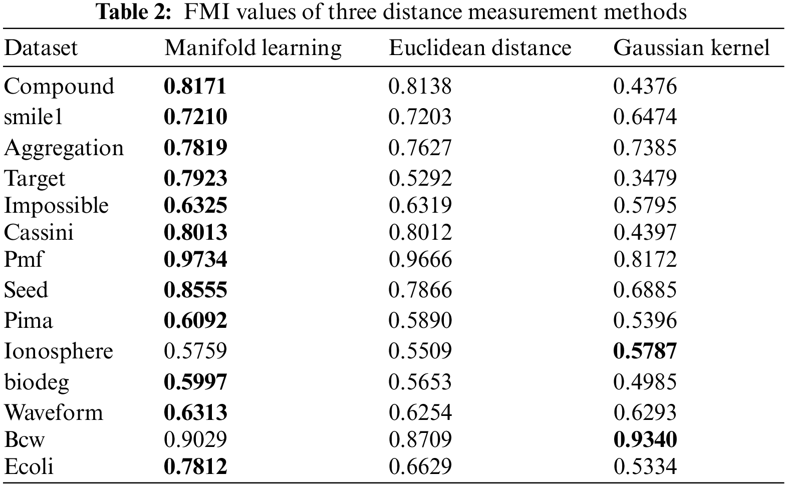
From the experimental results, it can be seen that Gaussian kernel function shows better FMI performance on data set Ionosphere and Bcw than Euclidean distance and manifold learning methods. However, in other cases, the manifold learning methods perform better in the FMI performance measures compared to the Euclidean distance and Gaussian kernel function, and the Gaussian kernel function performs worse in the FMI performance measures overall. In the seven low-dimensional artificial datasets, the manifold learning method improved the FMI performance metric by an average of 4.2% compared to the Euclidean distance and by an average of 21.99% compared to the Gaussian kernel function in the FMI performance metric. The distance measures of the manifold learning methods in the seven UCI high-dimensional datasets improve the FMI performance measures by an average of 4.35% compared to the Euclidean distance and by an average of 7.91% compared to the Gaussian kernel function. It can be seen that the Euclidean distance is still applicable in the clustering of high-dimensional data but it is not the optimal distance measure, and the manifold learning method is more suitable for clustering of high-dimensional data than the Euclidean distance and Gaussian kernel function.

5.4 Experiments on Artificial Dataset

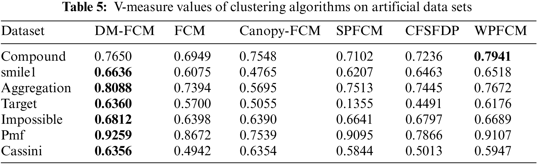
The performance of DM-FCM, FCM, Canopy-FCM, SPFCM, and CFSFDP on the seven artificial datasets are listed in Table 1. The clustering visualization results are shown in Figs. 2–8. DM-FCM algorithm can find out the suitable number of clusters and have better clustering effect in data with uneven density distribution, which also proves the effectiveness of improving local density in density Canopy algorithm. Canopy-FCM algorithm cannot find out the suitable number of clusters, but can roughly identify the class boundaries. SPFCM algorithm and FCM algorithm can complete a part of clustering, but The CFSFDP algorithm has the worst clustering effect. The visualization experimental results from Figs. 2–8 show that the DM-FCM algorithm has optimal clustering performance compared with other improved algorithms.

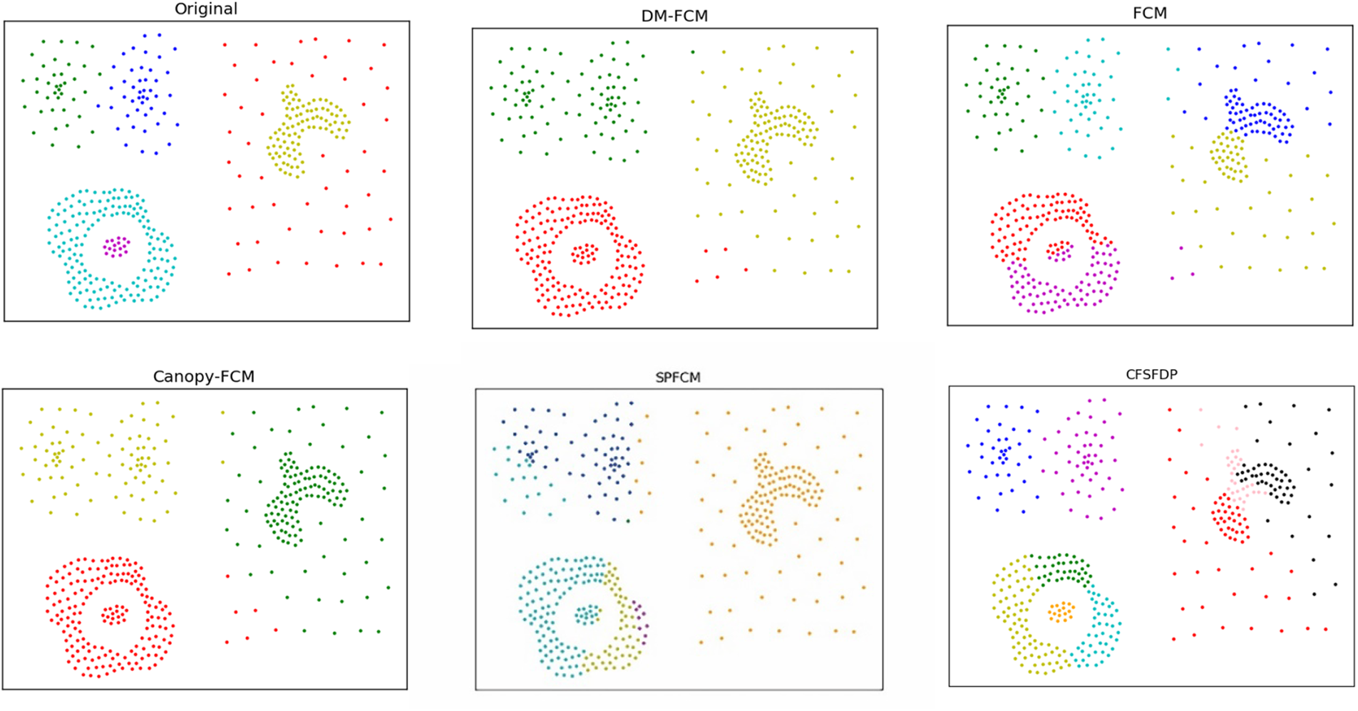
Figure 2: Clustering results of clustering algorithms on dataset compound

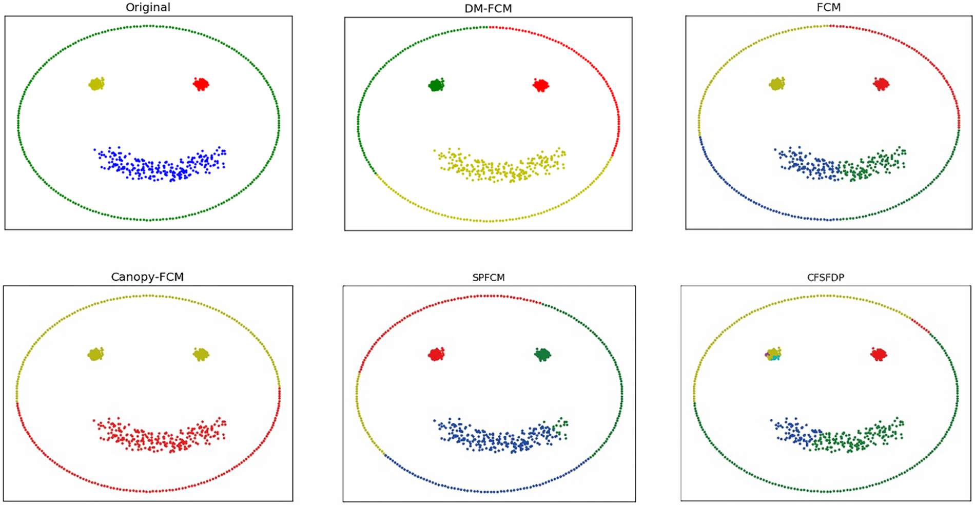
Figure 3: Clustering results of clustering algorithms on dataset smile1

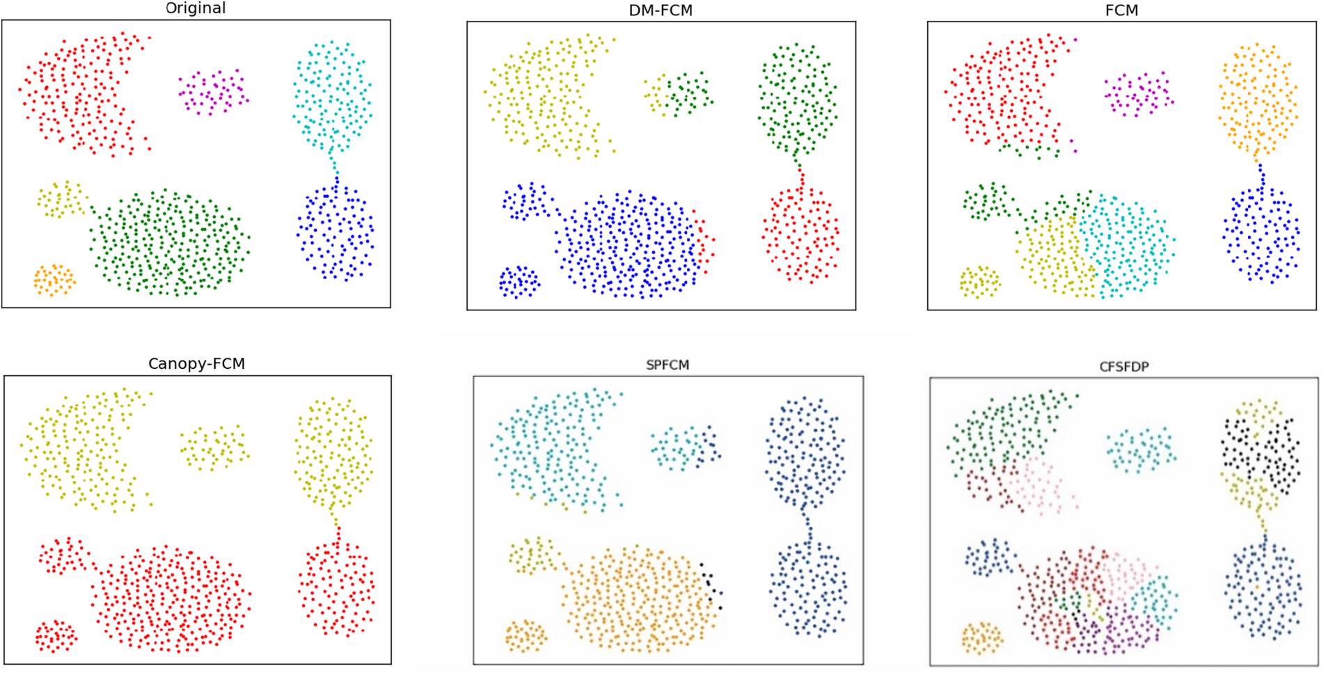
Figure 4: Clustering results of clustering algorithms on dataset aggregation

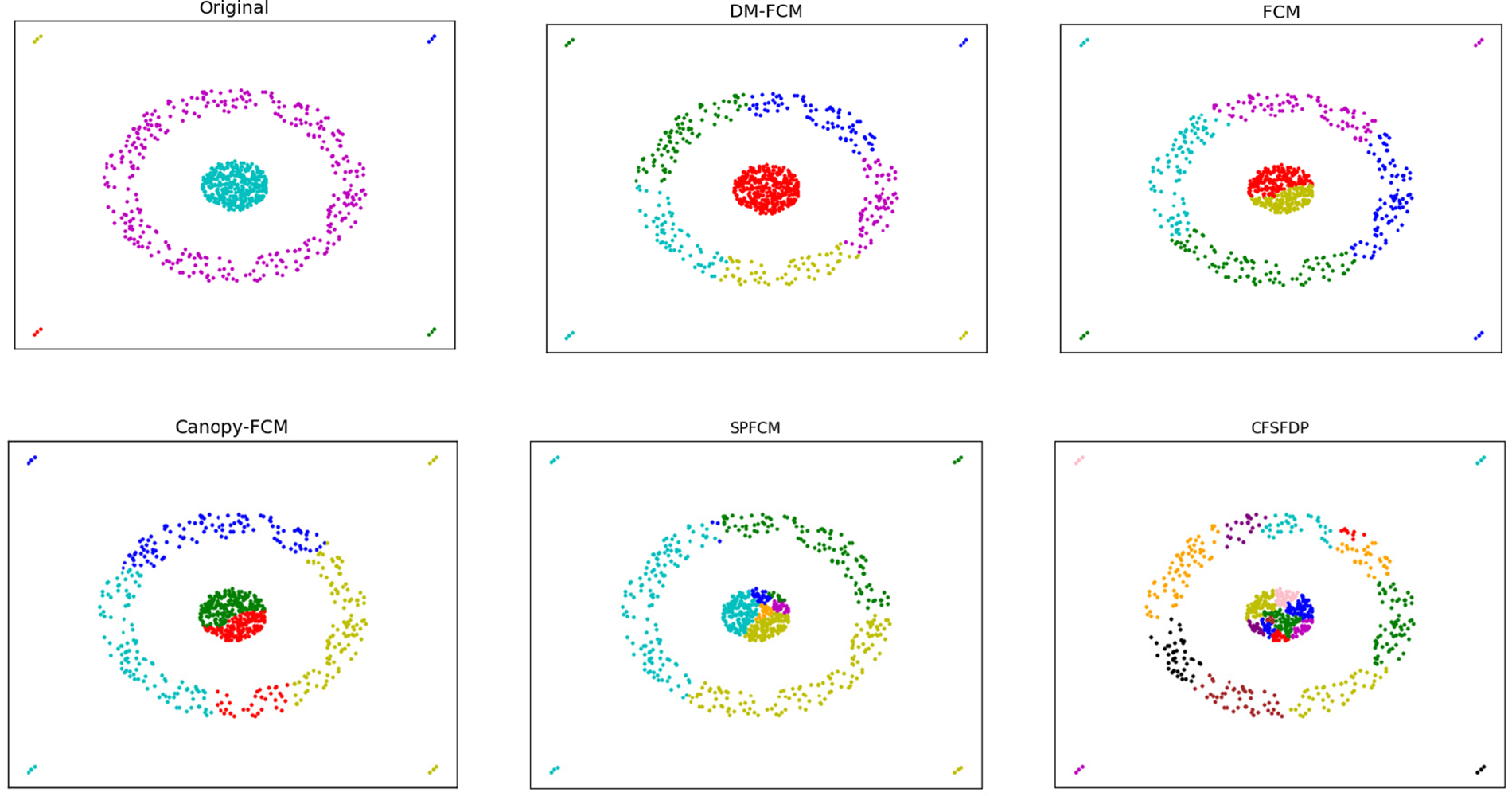
Figure 5: Clustering results of clustering algorithms on dataset target

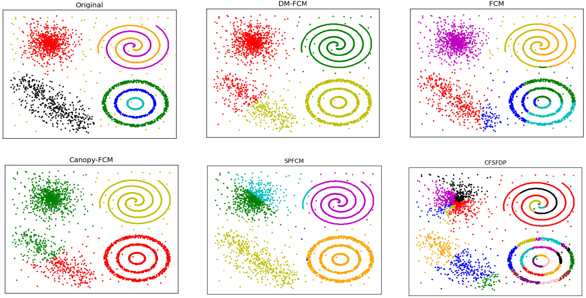
Figure 6: Clustering results of clustering algorithms on dataset impossible

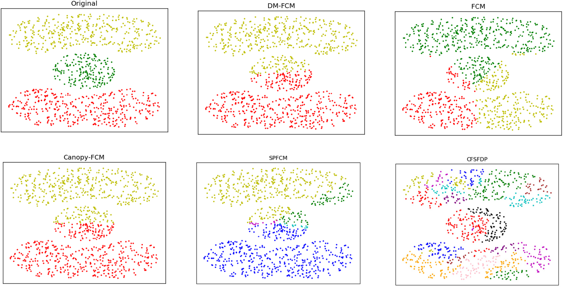
Figure 7: Clustering results of clustering algorithms on dataset cassini

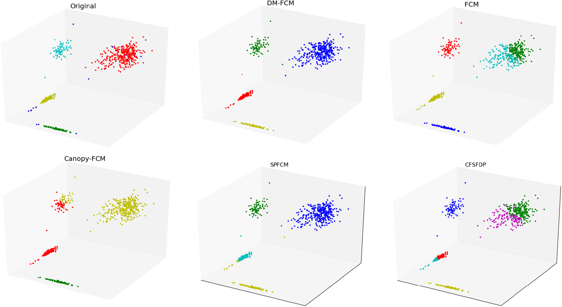
Figure 8: Clustering results of clustering algorithms on dataset Pmf

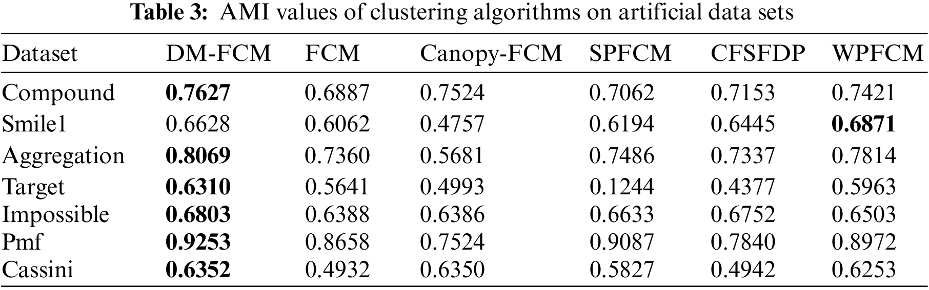
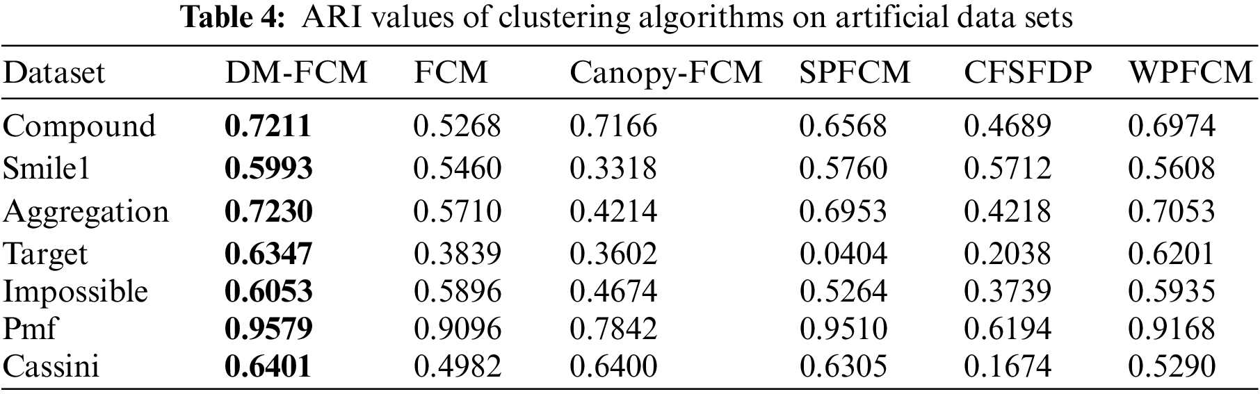
The DM-FCM algorithm improved the AMI performance metric by an average of 10.8%, the ARI performance metric by an average of 12.23%, and the V-measure performance metric by an average of 7.19% compared to FCM in the seven manual datasets. The average improvement in AMI performance metric, ARI performance metric, and V-measure performance metric is 11.18%, 16.57%, and 11.16%, respectively, compared to Canopy-FCM. DM-FCM has an average improvement of 10.73% in AMI performance measures, 11.5% in ARI performance measures, and 10.58% in V-measure performance measures compared to SPFCM. DM-FCM has an average improvement of 8.85% in AMI performance metrics, 29.36% in ARI performance metrics, and 8.36% in V-measure performance metrics compared to CFSFDP. The average improvement in AMI performance metric, ARI performance metric, and V-measure performance metric is 1.78%,3.69%, and 1.59%, respectively, compared to WPFCM. From the experimental results in Tables 3–5, it can be seen that the DM-FCM algorithm is the best in AMI, ARI, and V-measure performance measures compared to the Canopy-FCM algorithm, FCM algorithm, SPFCM algorithm, CFSFDP algorithm and WPFCM algorithm, and is superior in clustering of low-dimensional artificial datasets.

5.5 Experiments on the UCI Dataset

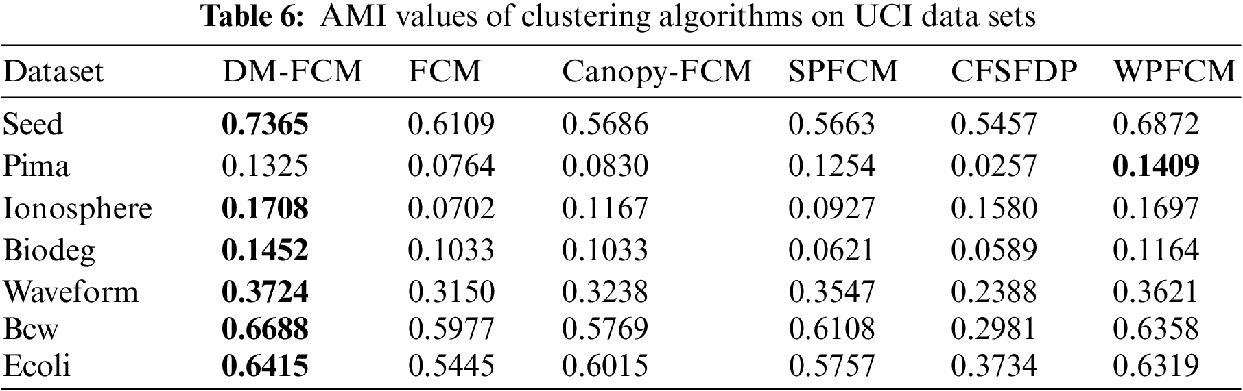
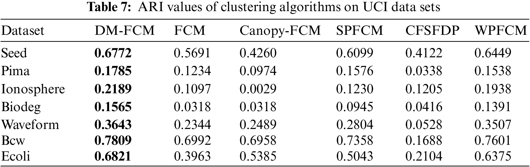
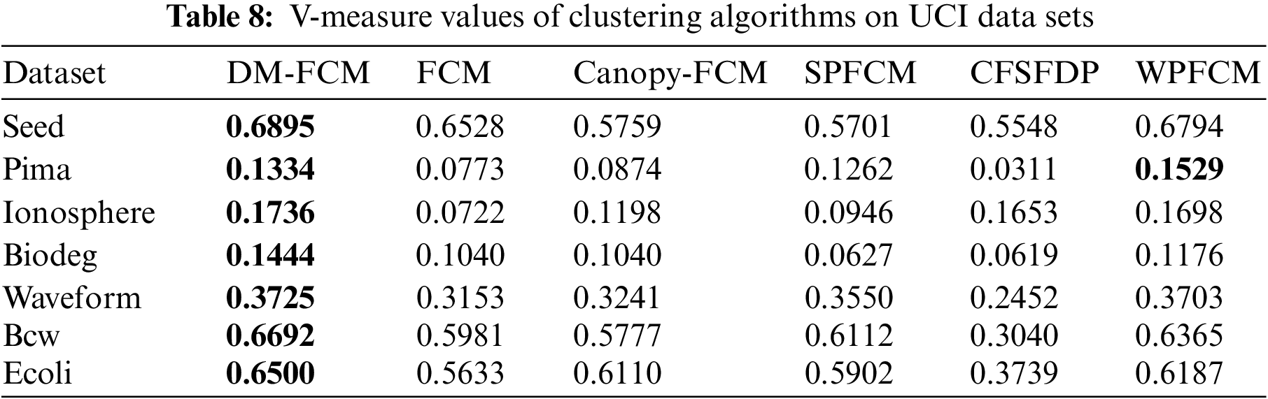
The experimental results in Tables 6–8 show that the DM-FCM algorithm has the best clustering performance in the six high-dimensional UCI datasets for the AMI, ARI, and V-measure performance measures. the DM-FCM algorithm improves on average by 7.85% in the AMI performance measure, 12.78% in the ARI performance measure, and 6.42% in the V-measure performance measure compared to the FCM algorithm. The DM-FCM algorithm improves the AMI performance metric by 7.06%, the ARI performance metric by 14.53%, and the V-measure performance metric by 6.18% on average compared to the Canopy-FCM algorithm. The DM-FCM algorithm improves the AMI performance metric by an average of 6.86%, the ARI performance metric by an average of 7.9%, and the V-measure performance metric by an average of 6.04% compared to the SPFCM algorithm. The DM-FCM algorithm improves on average by 16.7% in the AMI performance metric, 28.83% in the ARI performance metric, and 15.66% in the V-measure performance metric compared to the CFSFDP algorithm. the DM-FCM algorithm improves on average by 1.77% in the AMI performance measure, 2.55% in the ARI performance measure, and 1.25% in the V-measure performance measure compared to the WPFCM algorithm. Thus, the DM-FCM algorithm performs superiorly in clustering high-dimensional data.

5.6 Experiments on Runtime

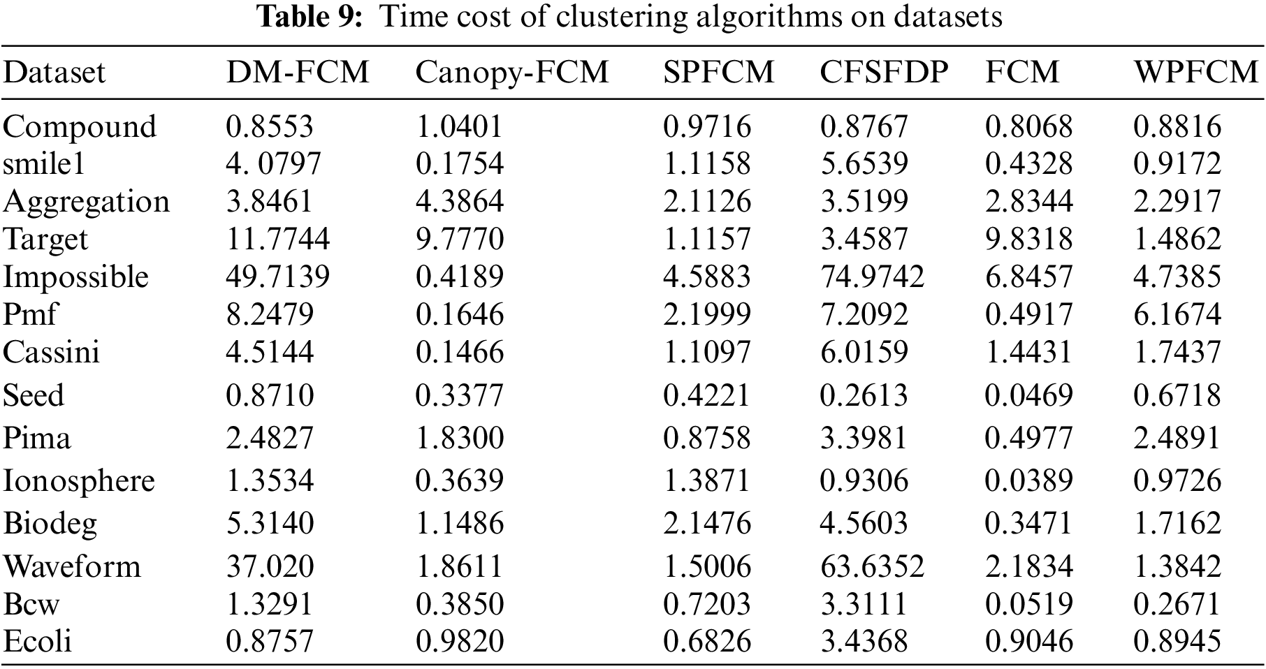
The running times of the 6 algorithms on 14 datasets were compared and the experimental results are shown in Table 9. Taking the running time of Compound on 6 algorithms as an example, the running time of DM-FCM algorithm on Compound dataset is 0.8553, and the algorithm with the lowest running time among the other comparison algorithms of non-FCM algorithms that is MD-FCM algorithm. The overall running time of DM-FCM is moderate compared to the other comparison algorithms because the MD-FCM algorithm requires adaptive selection of initial clustering centers using the density Canopy algorithm and optimization of the objective function using manifold learning, which increases the algorithm’s processing time for the dataset. From the running time of the six algorithms on 14 datasets and the clustering effect of the algorithms, it is clear that the DM-FCM algorithm does not have the best average running time compared to the other compared algorithms, but it performs significantly in improving the clustering effect.

6  Conclusions

To address the problem that the FCM algorithm easily falls into the local optimal solution and needs to determine the number of clusters in advance, the density Canopy algorithm based on improved local density is proposed to determine the number of clusters and initial cluster centers automatically. In addition, the actual complex high-dimensional data clustering becomes difficult in the era of big data, so manifold learning is introduced as the distance measure to optimize the clustering process. And the application of these methods is new and no researcher has combined these two methods before. The experimental results show that the DM-FCM algorithm produces very good clustering results on low-dimensional and high-dimensional data clustering without manually determining the number of clusters. Therefore, DM-FCM algorithm is more adaptive and stable, closer to the real structure of the manifold data distribution, and has better overall performance compared to the traditional FCM algorithm. Nevertheless, the computation time of this algorithm is long when dealing with large data sets, and how to decrease the computational complexity of the algorithm becomes the research direction of future work. The DM-FCM algorithm proposed in this paper has a wide range of applications in the research field of computer vision and image recognition. How to use the DM-FCM algorithm to improve the efficiency of practical applications in image processing is a problem that needs further research.

Acknowledgement: This work was funded by the National Natural Science Foundation of China and the Natural Science Foundation of Guangxi.

Funding Statement: The National Natural Science Foundation of China (No. 62262011), the Natural Science Foundation of Guangxi (No. 2021JJA170130).

Author Contributions: Study conception and design: H.W., J.C.; data collection: H.W.; analysis and interpretation of results: H.W., J.C. and X.X.; draft manuscript preparation: H.W., X.X. All authors reviewed the results and approved the final version of the manuscript.

Availability of Data and Materials: The URLs of the UCI datasets and artificial datasets supporting the results of this study are https://archive.ics.uci.edu/ml/datasets.php and https://github.com/milaan9/Clustering-Datasets, respectively.

Conflicts of Interest: The authors declare that they have no conflicts of interest to report regarding the present study.

References

1. C. C. Aggarwal and C. K. Reddy, “Data clustering,” in Algorithms and Applications. Londra: Chapman & Hall/CRC, 2014. [Google Scholar]

2. K. Wang, T. Zhang and T. Xue, “E-commerce personalized recommendation analysis by deeply-learned clustering,” Journal of Visual Communication and Image Representation, vol. 71, no. 6, pp. 102735, 2020. [Google Scholar]

3. H. Huang, F. Meng, S. Zhou, F. Jiang and G. Manogaran, “Brain image segmentation based on FCM clustering algorithm and rough set,” IEEE Access, vol. 7, pp. 12386–12396, 2019. [Google Scholar]

4. M. M. Ershadi and A. Seifi, “Applications of dynamic feature selection and clustering methods to medical diagnosis,” Applied Soft Computing, vol. 126, pp. 109293, 2022. [Google Scholar]

5. S. Demircan and H. Kahramanli, “Application of fuzzy C-means clustering algorithm to spectral features for emotion classification from speech,” Neural Computing and Applications, vol. 29, no. 8, pp. 59–66, 2018. [Google Scholar]

6. R. Xia, Y. Chen and B. Ren, “Improved anti-occlusion object tracking algorithm using Unscented Rauch-Tung-Striebel smoother and kernel correlation filter,” Journal of King Saud University-Computer and Information Sciences, vol. 34, no. 8, pp. 6008–6018, 2022. [Google Scholar]

7. J. C. Bezdek, Pattern Recognition with Fuzzy Objective Function Algorithms. Berlin, Germany: Springer Science & Business Media, 2013. [Google Scholar]

8. R. J. Kuo, T. C. Lin and F. E. Zulvia, “A hybrid metaheuristic and kernel intuitionistic fuzzy c-means algorithm for cluster analysis,” Applied Soft Computing, vol. 67, pp. 299–308, 2018. [Google Scholar]

9. Y. Ding and X. Fu, “Kernel-based fuzzy c-means clustering algorithm based on genetic algorithm,” Neurocomputing, vol. 188, pp. 233–238, 2016. [Google Scholar]

10. F. Silva and M. Telmo, “Hybrid methods for fuzzy clustering based on fuzzy c-means and improved particle swarm optimization,” Expert Systems with Applications, vol. 42, no. 17–18, pp. 6315–6328, 2015. [Google Scholar]

11. X. Liu, J. Fan and Z. Chen, “Improved fuzzy c-means algorithm based on density peak,” International Journal of Machine Learning and Cybernetics, vol. 11, no. 3, pp. 545–552, 2020. [Google Scholar]

12. H. Bei, Y. Mao and W. Wang, “Fuzzy clustering method based on improved weighted distance,” Mathematical Problems in Engineering, vol. 2021, no. 5, pp. 1–11, 2021. [Google Scholar]

13. J. Chen, H. Zhang and D. Pi, “A weight possibilistic fuzzy C-means clustering algorithm,” Scientific Programming, vol. 2021, no. 15, pp. 1–10, 2021. [Google Scholar]

14. Y. Liu, Y. Zhang and H. Chao, “Incremental fuzzy clustering based on feature reduction,” Journal of Electrical and Computer Engineering, vol. 2022, no. 2, pp. 1–12, 2022. [Google Scholar]

15. B. Cardone and F. Di Martino, “A novel fuzzy entropy-based method to improve the performance of the fuzzy C-means algorithm,” Electronics, vol. 9, no. 4, pp. 554, 2020. [Google Scholar]

16. S. Surono and R. D. A. Putri, “Optimization of fuzzy c-means clustering algorithm with combination of minkowski and chebyshev distance using principal component analysis,” International Journal of Fuzzy Systems, vol. 23, no. 1, pp. 139–144, 2021. [Google Scholar]

17. Y. Zhang, X. Bai and R. Fan, “Deviation-sparse fuzzy c-means with neighbor information constraint,” IEEE Transactions on Fuzzy Systems, vol. 27, no. 1, pp. 185–199, 2018. [Google Scholar]

18. L. Tang, C. Wang and S. Wang, “A novel fuzzy clustering algorithm based on rough set and inhibitive factor,” Concurrency and Computation: Practice and Experience, vol. 33, no. 6, pp. e6078, 2021. [Google Scholar]

19. Z. Pawlak, “Rough sets,” International Journal of Computer & Information Sciences, vol. 11, no. 5, pp. 341–356, 1982. [Google Scholar]

20. J. C. Fan, Y. Li and L. Y. Tang, “RoughPSO: Rough set-based particle swarm optimization,” International Journal of Bio-Inspired Computation, vol. 12, no. 4, pp. 245–253, 2018. [Google Scholar]

21. Y. Gao, Z. Wang and H. Li, “Gaussian collaborative fuzzy c-means clustering,” International Journal of Fuzzy Systems, vol. 23, no. 7, pp. 2218–2234, 2021. [Google Scholar]

22. D. Muhammet, D. Pamucar, I. Gokasar, M. Köppen and B. B. Gupta, “Personal mobility in metaverse with autonomous vehicles using Q-rung orthopair fuzzy sets based OPA-RAFSI model,” in IEEE Transactions on Intelligent Transportation Systems, USA: IEEE, pp. 1–10, 2022. [Google Scholar]

23. J. R. Alharbi and W. S. Alhalabi, “Hybrid approach for sentiment analysis of Twitter posts using a dictionary-based approach and fuzzy logic methods: Study case on cloud service providers,” International Journal on Semantic Web and Information Systems (IJSWIS), vol. 16, no. 1, pp. 116–145, 2020. [Google Scholar]

24. M. A. Alsmirat and Y. Jararweh, “Accelerating compute intensive medical imaging segmentation algorithms using hybrid CPU-GPU implementations,” Multimedia Tools and Applications, vol. 76, pp. 3537–3555, 2017. [Google Scholar]