Research on Total Electric Field Prediction Method of Ultra-High Voltage Direct Current Transmission Line Based on Stacking Algorithm

1  Introduction

Ultra-high voltage (UHV) DC transmission lines have the advantage of transferring information over long distances and with higher power compared to general lines. Although general lines facilitate residential and industrial electricity consumption, they are often associated with electromagnetic environmental impacts, such as the total electric field and audible noise [1]. The ground electric field of DC transmission lines is named DC total electric field. As the transmission frequency is 0 Hz, the space charge, generated by the corona of the wire during line operation, produces air ions, and the superposition of the ion flow field and the nominal electric field of the wire itself will significantly increase the strength of the ground total electric field [2]. The total electric field on the ground can negatively affect people’s lives, mainly the problem of how people feel underneath the DC lines. Possible effects are the feeling of people under the synthetic electric field and the feeling of the human body intercepting the ion flow. By the China Electric Power Research Institute, experimental proof: human hair and skin are the most sensitive to the synthetic electric field, when the electric field strength of 30, 35, 38, and 44 kV/m, human exposed skin will feel a weak tingling sensation, more obvious tingling sensation, very obvious tingling sensation, and strong tingling sensation, respectively. If you leave the high-intensity area of the synthetic electric field, the irritation will disappear immediately. Therefore, the relevant industry standards specify that the total ground electric field of DC transmission lines needs to be controlled below 30 kV/m [3]; the total electric field limits for ±800 kV extra-high voltage (EHV) transmission lines are 30 and 25 kV/m in less populated areas and residential areas, respectively, under clear conditions [4].

2  Related Work

The total electric field has been the subject of substantial studies performed by national and international scientists. The total electric field distribution of bipolar DC transmission lines is being calculated abroad, based on the Deutsch or Kaptzov hypothesis [5,6], while the electromagnetic environment of UHV transmission lines has been extensively investigated in China, using the finite element method [7]. With the development of computer technology [8], the research has become more insightful and the calculation model has extended from two-dimensional to three-dimensional [9]. The analysis and calculation of the total electric field have evolved to consider different structures of EHV lines e.g., UHV co-tower double-return DC lines, AC-DC parallel lines, cross-span DC lines, and critical obstacles under the transmission lines, including human bodies and buildings [10]. The effects of complex environmental factors such as high altitude [11], air humidity, and airborne particulate matter, on the total electric field at ground level, have also started to emerge. The spectral element method is a new international numerical calculation method, which has obvious advantages in the calculation accuracy and calculation speed compared with the finite element method. For example, the spectral element method, as an extension of the finite element method, is used in electromagnetic scattering problems to demonstrate its high accuracy [12] and to use its high accuracy for conjectural proofs in other scientific studies [13]. However, the numerical calculation of this multi-physics field fusion in China is still mainly done by the finite element method. The finite element method adopted in China fails to fully reflect the influence of complex environmental factors on the total electric field. These factors include temperature, humidity, wind direction, varied sizes of airborne particulate matter, and wind speed.

Local outlier factor algorithm (LOF), density-based clustering algorithm (DBSCAN), and Isolation Forests are widely used in various fields of scientific research. The clustering quality is poor if the density of the sample set is not uniform and the clustering spacing difference is very different. The algorithm is more complex than traditional clustering algorithms in terms of adjusting parameters, and different parameters have a greater impact on the clustering results. The advantage of the isolated forest algorithm is that it does not use distance or density metrics to detect anomalies, which eliminates the cost of distance calculation in all distance-based and density-based methods, the isolated forest algorithm has linear time complexity, low constants, and low memory requirements, and converges quickly. However, the dimensionality of the data in the training of this algorithm is random, which will cause a large amount of useless noise, when the sample size is too much, it may cause the normal samples near the anomalous samples, affecting the classification process. LOF is a generally applicable outlier processing algorithm, compared to other outlier processing algorithms method is more concise and easier to operate and will not be affected by the distribution of the data itself. For example, it has good performance in anomalous electricity consumption data and financial risk data. This is more friendly to the measured data of ground synthetic electric field. In this paper, we employ the original data collected from the Ningdong-Zhejiang ±800 kV UHVDC transmission project. The collected data are firstly removed from the outliers based on the Local outlier factor (LOF) algorithm; then the base learner is trained by a five-fold cross-validation, and the algorithm model is trained by seven features, namely temperature, humidity, air pressure, wind speed, PM10, PM2.5 and PM1.0. The Mean Square Error (MSE), Root Mean Square Error (RMSE) and Mean Absolute Error (MAE) were used to quantify the accuracy of the prediction outcomes. These prediction outcomes were compared with the traditional finite element method to verify the effectiveness of the Stacking algorithm in UHVDC transmission lines.

3  The Acquisition of Total Electric Field Data

To study the influence of complex meteorological factors outside the room, on the total electric field on the ground of the UHVDC transmission line, the Ningdong-Zhejiang ±800 kV UHVDC transmission project (Ling Shao line) was selected according to the national measurement standard DL/T 1089–2008, and the total electric field data collection and meteorological data were carried out between pole towers #1951 and #1952 in Xinyang, Henan Province. As shown in Fig. 1, the ground area is open and flat. The main crop in the farmland below the measurement point line is a low crop of wheat. A few farmers are living around that can provide power for the measurement equipment and there are no other lines or obstacles near the measurement point to interfere with the data collection.

Figure 1: The satellite map of the measurement location

The process of data collection is shown in Fig. 2. The equipment for data collection is by the standards set by the China Electricity Association. The total electric field was continuously monitored by 27 Traffic Flow Management System (TFMS) field wear probes positioned below the cross-section of the EHV transmission line, with an accuracy level of 5%. Probe No. 10 was located below the positive pole of the transmission line and probe No. 17 was located below the negative pole of the transmission line. The Engineering Workstation (EWS) collected the meteorological data, from Wuhan Purple Forain Technology Co., Ltd., China. Electric field data was collected every 10 s and meteorological data was collected every 1 min, and each data collection process lasted for three days.

Figure 2: Measurement location illustrating the (a) ground view of the metal plate and electric field meter position, and (b) top view illustrating the negative and positive pole of the transmission line as well as the environmental monitoring location and electric field meter

4  Analysis of Abnormal Data

4.1 Detection of Univariate Outliers

Abnormal data can be acquired due to external environmental disturbances during the data collection process. Take univariate time series data from probes No. 10 and No. 17 as an example. In Fig. 3, at around 20:39 and 20:55, on May 27, the points marked by red circles at around 23:20 are numerically much smaller, or larger, than the average value, and there are no points of comparable size near such numerical jump points-which are thought as outliers in the data set. However, we can see from the graph that there are also a few points where the values slightly fluctuate, which could be considered outliers as well.

Figure 3: Univariate outliers

4.2 Detection of Multivariate Outliers

The correlation analysis of the data collected by each probe, as shown in Fig. 4, shows that the Pearson correlation coefficients between probes with similar locations are generally large, and there is a relatively strong linear relationship between the data collected by each probe. An increase in the number of variables leads to more prominent outliers.

Figure 4: Pearson correlation coefficient of adjacent probes

The bivariate outliers were determined as shown in Fig. 5. Two sets of data were selected for analysis, (a) a bivariate scatter plot made from the measured data of probe No. 10 and probe No. 11 at 21:00 on May 27, 2021, which are more correlated, and (b) a bivariate scatter plot made from the measured data of probe No. 13 and probe No. 17 at 2:00 on May 28, 2021, which are less correlated. Points marked by dashed-red circles are obvious outliers.

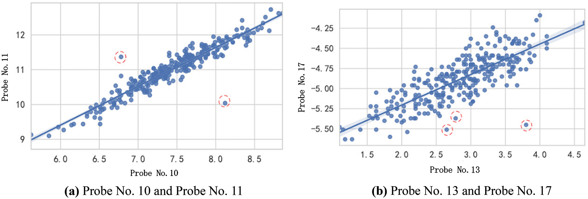
Figure 5: Bivariate outliers

The determination of multivariate anomalies is shown in Fig. 6. Two sets of data are selected: (a) the 3D scatter plot made by the measurement data of probes No. 1, No. 2, and No. 4 at 2:00 on May 28, 2021, with stronger correlation, and (b) is the 3D scatter plot made by the measurement data of probes No. 1, No. 8, and No. 12 at 21:00 on May 27, 2021, in which the points marked by dashed-red circles are obvious outliers. From Figs. 5 and 6, the outliers in the (a) plot with the stronger correlation of variables, are clearer, and the outliers in the (b) plot with a weaker correlation, are less clear, with some points that are difficult to discriminate. Hence, the variables with stronger correlation should be selected for the determination of multivariate outliers. By observing the time series line graph, two-dimensional scatter plot, and three-dimensional scatter plot of total electric field data, we found that the difference between normal data and abnormal data was enlarged when the number of variables increased, and the variables with stronger correlation should be selected for the determination of abnormal values.

Figure 6: Three-variable outlier

4.3 Multivariate-Based Outlier Determination Method

The analysis in Section 3 shows that multivariate outlier detection methods are more effective. The LOF algorithm is an unsupervised algorithm for determining outliers in multivariate data. It quantifies the degree of anomalies at each point in the data set by calculating the distance and density. We note that in this paper, there is a strong linear relationship between the data collected by each probe. Thus, the distance between points is calculated using the Euclidean distance. The kth distance of a point p in the dataset is given by:

dk(p)=d(p,o)(1)

where: d(p,o) is the distance between point p and point o. There are at least k points in the data set other than p whose distance to point p is less than or equal to d(p,o), and at most k-1 points other than p whose distance to point p is less than or equal to d(p,o).

The kth distance neighbourhood of a point p in the dataset is:

Nk(p)={q∈D\{p}|d(p,q)≤dk(p)}(2)

where: point q is in the domain of point p; D\{p} is all points outside of point p. The reachable distance from point o to point p in the dataset is:

Rdk(p,o)=max{Nk(o),d(p,o)}(3)

The local reachable density of a point p in the dataset is:

lrdk(p)=1/(∑o∈Nk(p)Rdr(p,o)|Nk(p)|)(4)

The local anomaly factor for a point p in the dataset is:

LOFk(p)=∑o∈Nk(p)lrdk(o)lrdk(p)|Nk(p)|(5)

When the value of the local anomaly factor is close to 1, the density of point p is close to that of the neighboring points, and point p is a normal point; when the value of the local anomaly factor is less than 1, the density of point p is larger, and point p is a normal point; If the value of the local anomaly factor is greater than 1, the density of point p is smaller and relatively far from the cluster where other points are gathered, so the larger the local anomaly factor, the more likely point p is an anomaly.

4.4 The Result of Removing Outliers

LOF, DBSCAN, and isolated forest are all multivariate outlier detection methods. In the process of outlier determination, the algorithms used are prone to overfitting leading to the deletion of valid data, and using accuracy alone does not present a comprehensive picture of the determination accuracy of each algorithm model. The confusion matrix is shown in Fig. 7, TP is True & Positive: the number of actual samples that are valid and classified as valid; FP is False & Positive: the number of actual samples that are abnormal and classified as valid; FN is False & Negative: the number of actual samples that are valid and classified as abnormal; TN is True & Negative: the number of actual samples are abnormal data and classified as abnormal data. From the confusion matrix, more accurate classifier evaluation metrics can be further obtained. In this paper, three evaluation metrics are used, which are precision, recall, and F1-score.

Figure 7: Confusion matrix

The accuracy rate P refers to the proportion of samples that are determined by the algorithm to be valid and are valid out of the total number of samples determined by the algorithm to be valid:

P=TPTP+FP(6)

Recall R refers to the proportion of samples that are determined by the algorithm to be valid data and are valid data out of the actual valid data samples:

R=TPTP+FN(7)

The F1-score metric combines the output results of accuracy and recall. F1-score takes values from 0 to 1, where 1 represents the best output result of the model and 0 represents the worst output result of the model and is calculated according to the following formula:

F1−score=2PRP+R(8)

As shown in Table 1, the accuracy of the isolated forest algorithm is the highest among the three methods, reaching 99.35%, indicating that the algorithm eliminates invalid data very cleanly, but the final recall rate and F1-score are low, indicating that many valid data are mistakenly deleted in the eliminated data. The method has the best overall effect and is more suitable for the determination of the anomalous values of the synthetic electric field of transmission lines than the other three methods.

5  The Prediction of DC Transmission Line Total Electric Field

At present, the ground total electric field prediction methods of DC lines mainly include calculation methods based on the Deutsch assumption, the up-flow finite element method, and the flux line method. However, the actual UHV transmission lines in China go through several provinces and cross complex and variable terrain In addition, the total electric field is easily affected by meteorological factors, while the traditional numerical calculation methods are difficult to fully consider the influence mechanism of the complex environment on the total electric field, such as temperature, humidity, wind direction, different particle sizes of airborne particles and wind speed. All the above-mentioned factors make it difficult to effectively predict the total electric field. Compared with the traditional total electric field prediction method, the machine learning-based prediction method can better consider the influence of a complex environment on the total electric field on the ground. Compared with a single machine learning algorithm, the stacking algorithm can further improve the prediction accuracy and avoid overfitting or underfitting the prediction model.

5.1 The Superposition Prediction Model of DC Transmission Line Total Electric Field

The Stacking framework is an integrated learning model with a serial structure proposed by WOLPERT [14]. Unlike integrated learning methods such as Bagging, Boosting, and Voting, the meta-learner, in the second layer of Stacking, uses the output of multiple base learners. As shown in Fig. 8, we selected the RandomForest, GBDT, LightGBM, XGBoost, and KNN as the base learners, and a linear regression model as the meta-learners, in the second layer for the final prediction [15]. Since the total electric field is influenced by numerous environmental factors, the usage of multiple linear regression for electric field prediction is more realistic, convenient, and fast.

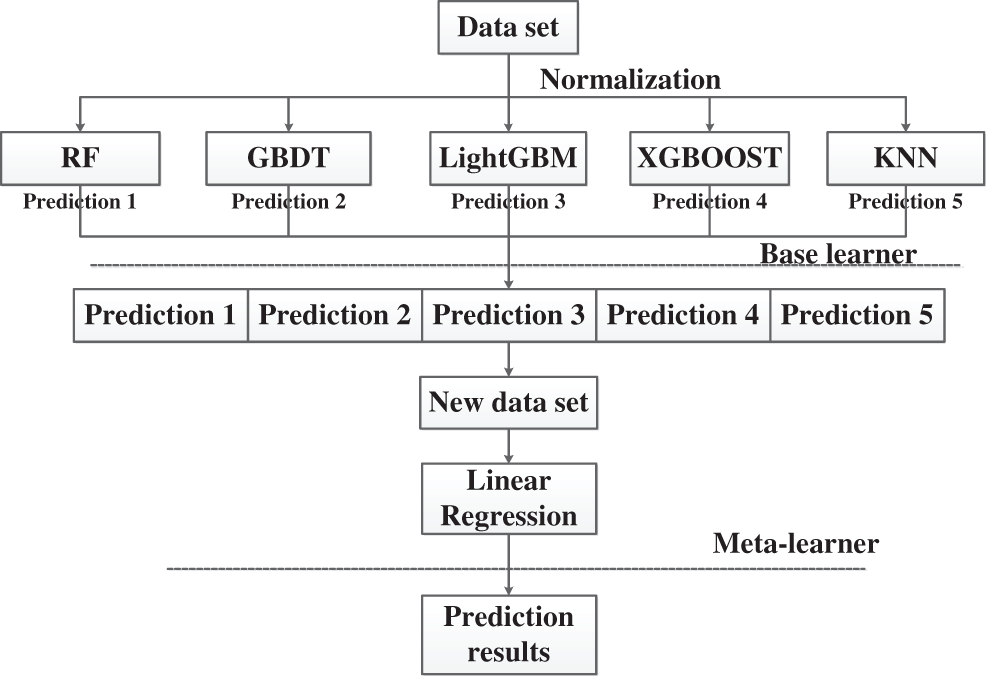
Figure 8: Framework of Stacking integrated learning model

The training steps of the Stacking framework used in this paper are as follows:

(1)   Normalizing the initial data to obtain a data set as G={(yi,xi);i=1,2,…,m}, where xi is the characteristic vector of the ith sample and yi is the predicted value corresponding to the ith sample.

(2)   The data G is divided into a training set Gtrain and a testing set Gtest. The basic learner of the first layer is trained by 50% cross-validation for Gtrain. Eq. (6) is obtained by equally dividing Gtrain into five parts:

Gtrain=Gtrain1+Gtrain2+Gtrain3+Gtrain4+Gtrain5(9)

One fold is selected as the test set and the remaining four folds are selected as the training set. The prediction result of a base learner Hk,k=1,…,K, in the five training processes, can be expressed as zkn. The final output results of K base learners and yn of Gtrain form a new training set, used by the second-level meta-learners as:

Gtrain−new={(yn,z1n,…,zKn);n=1,…,N}(10)

(3)   In step (2), during the five-fold cross-validation, the basic learners Hk will be trained once for each cross-validation, and yi out of Gtest will be predicted by each trained Hk. Finally, after the five-fold cross-validation, the predicted value Pkn, of each basic learner output Gtest is shown in Eq. (8):

Pkn=(Pkn1+Pkn2+Pkn3+Pkn4+Pkn5)/5(11)

The results of the final K basic learners and yi out of Gtest, form a new test set for the second level meta-learners as given by Eq. (9):

Gtest−new={(yn,P1n,⋯,PKn);n=1,…,N}(12)

(4)   The meta-learner of the second layer is trained by Gtrain−new, and the accuracy of the model is tested by Gtest−new.

To maximize the prediction accuracy of the linear regression algorithm, of the meta-learner in the second layer, the five prediction algorithms RandomForest [16], GBDT [17], LightGBM [18], XGBoost [18], and KNN [19], which have a high learning ability and large structural differences, were selected for the base learner in the first layer. We note that XGBoost [20], LightGBM, and GBDT are different implementations of the Boosting integrated learning method based on decision trees; RandomForest is an implementation of the Voting integrated learning method based on decision trees; and KNN is a machine learning method that calculates distances in the feature space, which is relatively mature in both theory and application [21].

The detailed process of 5-fold cross-validation in steps (2) and (3) is shown in Fig. 9. The general steps are: 1) divide the dataset into five parts, one of which is the test set and the remaining four are the training set; 2) repeat step (1) five times, respectively, with different test sets selected each time; 3) use the dataset predicted by the base learner as the training set and test set of the meta-learner. However, this approach is likely to lead to overfitting of the prediction results, so this research paper combines the initial data set with the predicted data set of the base learner as the training set and test set of the meta-learner, which can effectively avoid overfitting or underfitting of the model. Five-fold cross-validation can effectively avoid model overfitting or underfitting.

Figure 9: The five-fold cross-validation

5.2 Comparison of Prediction Results

In this paper, the algorithm model is trained to predict the ±800 kV transmission line ground total electric field by seven features: temperature, humidity, air pressure, wind speed, PM10, PM2.5, and PM1.0.

The meteorological data points of the total electric field are normalized by Eq. (10). To improve the predictive accuracy, values are converted between 0 and 1 to avoid the impact of the difference in magnitude between different features.

S=s−sminsmax−smin(13)

In Eq. (10), S is the result of the normalization of each feature; s is the original data of each feature; Smax and Smin are the maximum and minimum values of each feature.

To further improve the prediction outcome, due to the random arrangement and combination of data when dividing the training set and the test set, we divided the data set into four training sets and one test set, using five-fold cross-validation [22]. We quantified the error of the model prediction results by Mean Square Error (MSE), Root Mean Square Error (RMSE), and Mean Absolute Error (MAE), as in Eqs. (11)–(13) [23]. A smaller error means a better prediction. Additionally, the final result is the average of five predictions.

MSE=1n∑i=1n(yi−y^i)2(14)

RMSE=1n∑i=1n(yi−y^i)2(15)

MAE=1n∑i=1n|yi−y^i|(16)

In Eqs. (11) to (13), yi and y^i represent the real values and predicted values, respectively; n represents the number of predicted values and real values.

In this paper, two experimental data sets in May 2021 and November 2021 were selected as prediction datasets. These two experiments have different environment variables, and the prediction results of the Stacking algorithm are compared with the single prediction results of the selected five base learners, as shown in Tables 2 and 3.

From Tables 2 and 3, each single machine learning algorithm has its advantages and disadvantages. The MSE, RMSE, and MAE errors, of the Stacking algorithm, are lower than those of other prediction algorithms and are therefore more suitable for the prediction of the total electric field of transmission lines.

5.3 Comparison of the Stacking Algorithm with the Traditional Finite Element Method

According to the specific parameters of the “Ling Shao line” in Table 4, we conducted finite element simulation and compared the simulation results, the predicted results of the Stacking algorithm with the measured total electric field.

The finite element model is shown in Fig. 10. To reduce the calculation error and improve efficiency, in the modeling of the artificial boundary, we added a layer of infinite element domain. Infinite elements can simulate an infinite space. The infinite element and artificial boundary radius difference is set to 10 m. We use the coordinate scaling method to expand the calculation domain 1000 times. We note that the calculation domain radius is 10 × 103 m. The expansion makes the finite element calculation model close to the actual open domain. This fits the FEM model to the actual open domain and reduces computational errors. When dissecting the model’s mesh, the air domain uses an extremely refined triangular mesh with a minimum mesh length. The minimum mesh length is set to a smaller value than the equivalent radius of the transmission line. The infinite element domain also uses a more refined mesh structure with radial mapping [24]. After the mesh division method, the quality of the model mesh division was improved, and the number of mesh sections was reduced, effectively improving the computational efficiency [25].

Figure 10: Finite element calculation model for ±800 kV DC transmission line

5.4 Comparative Analysis

The simulation comparison between the traditional finite element method, the prediction results of the Stacking algorithm, and the measured total electric field are compared and analyzed in Fig. 11.

Figure 11: Comparison between the finite element method simulation, the Stacking algorithm simulation, and the measured total electric field

The total electric field calculated by the finite element method shows a uniformly symmetrical curve. The positive side and the measured field strength of the negative side of the data exhibit a good fit. The positive side shows a maximum error of 16.1%. The negative side of the data is notoriously shifted, and the maximum field strength error is 44.37%; The Stacking algorithm predictions of the field strength and the measured field strength of the positive and negative sides of the trend are well aligned. The maximum error on the positive side is 13.8%. The maximum field strength error on the negative side is 14.1%. Therefore, the prediction error of the Stacking algorithm is less than the error of the traditional finite element method.

6  Conclusion

The total electric field data collection process is complicated and susceptible to environmental factors. The existence of outliers in the collected data set could significantly affect the final prediction outcome. Identification and elimination of the outliers is therefore a crucial step in the data pre-processing. In this work, we compare and analyze three multivariate outlier rejection algorithms, namely LOF, DBSCAN, and Isolation Forests, and conclude that the mean change of each percentile difference in the data set is relatively small after using the LOF algorithm to eliminate the outliers Thus, the LOF algorithm is chosen to detect the outliers in the total electric field data set.

After eliminating the outliers in the total electric field data set, the Stacking algorithm is chosen to predict the total electric field. By comparing the prediction results of the May and November data sets, The Stacking algorithm exhibits a smaller prediction error and is more accurate than other prediction algorithms. In addition, after comparing the total electric field prediction outcomes of the Stacking algorithm with the traditional finite element method, the Stacking prediction algorithm reveals more accuracy. Also, the prediction outcome is more in line with the actual change law. The Stacking algorithm can effectively conduct the prediction of the total electric field on the ground, of the UHVDC transmission line, and could be a valuable tool to avoid safety hazards and ensure a stable operation of the transmission line.

Acknowledgement: This work was funded by a Science and Technology Project of State Grid Corporation of China, and the European Research Council (ERC) under the European Union’s Horizon 2020 Research and Innovation Program.

Funding Statement: This work was funded by a science and technology project of State Grid Corporation of China “Comparative Analysis of Long-Term Measurement and Prediction of the Ground Synthetic Electric Field of ±800 kV DC Transmission Line” (GYW11201907738). Paulo R. F. Rocha acknowledges the support and funding from the European Research Council (ERC) under the European Union’s Horizon 2020 Research and Innovation Program (Grant Agreement No. 947897).

Author Contributions: The authors Yinkong Wei, Mucong Wu, and Ziyi Cheng processed the measured synthetic electric field data with anomalies, analyzed the influence of meteorological factors on the synthetic electric field at the ground level, and subsequently predicted accurately the synthetic electric field values at different locations on the ground level, in which the author Yinkong Wei participated in the whole field experiment and all the algorithms, and the author Mucong Wu contributed in the processing of the synthetic field anomalies, and the author Ziyi Cheng contributed in the analysis of meteorological factors and prediction of synthetic electric field values at different locations on the ground level. Author Ziyi Cheng contributed to the analysis of meteorological factors and the prediction of synthetic electric field values at different locations on the ground. Authors Wei Wei and Weifang Yao provided the test site and measurement equipment for the field test of the synthetic electric field and meteorological conditions. Author Paulo R. F. Rocha contributed to the language revision of the paper.

Availability of Data and Materials: Not applicable.

Conflicts of Interest: The authors declare that they have no conflicts of interest to report regarding the present study.

References

1. A. Alassi, S. Banales, O. Ellabban, G. Adam and C. Maciver, “HVDC transmission: Technology review, market trends and future outlook,” Renewable and Sustainable Energy Reviews, vol. 112, pp. 530–554, 2019. [Google Scholar]

2. X. Q. Ma, K. He, J. Y. Lu, L. Xie, Y. Ju et al., “Effects of temperature and humidity on ground total electric field under HVDC lines,” Electric Power Systems Research, vol. 190, pp. 1–8, 2021. [Google Scholar]

3. China National Development and Reform Commission, Limit Values of Electromagnetic Environment Parameters for 800 kV Extra-High Voltage DC Lines: DL/T1088-2008. Beijing, China: China Electric Power Press, 2008. [Google Scholar]

4. China National Development and Reform Commission, Design Specifications for ±800 kV DC Overhead Transmission Lines: GB/T50790-2013. Beijing, China: China Planning Press, 2013. [Google Scholar]

5. M. P. Sarma and W. Janischewskyj, “Analysis of corona losses on DC transmission lines: I-unipolar lines,” IEEE Transactions on Power Apparatus and Systems, vol. PAS-88, no. 5, pp. 718–731, 1969. [Google Scholar]

6. M. P. Sarma and W. Janischewskyj, “Analysis of corona losses on DC transmission lines part II-bipolar lines,” IEEE Transactions on Power Apparatus and Systems, vol. PAS-88, no. 10, pp. 1476–1491, 1969. [Google Scholar]

7. M. Xie, L. Xie, K. He and J. Lu, “Research on 3-D total electric field of crossing high voltage direct current transmission lines based on upstream finite element method,” High Voltage, vol. 6, no. 1, pp. 160–170, 2021. [Google Scholar]

8. J. H. Kim, S. Joo and Y. S. Chung, “Improved flux tracing method based on parametric curve for calculating ion flow field of HVDC transmission lines,” IEEE Access, vol. 9, pp. 105724–105732, 2021. [Google Scholar]

9. L. Hao, L. Xie, B. Bai, T. Lu and X. Li, “High effective calculation and 3D modeling of ion flow field considering the crossing of HVDC transmission lines,” IEEE Transactions on Magnetics, vol. 56, no. 3, pp. 1–5, 2020. [Google Scholar]

10. S. X. Li, D. L. Wang and T. B. Lu, “Characteristics of electrostatic discharges between metallic objects in the ion-flow field under HVDC lines,” The Journal of Engineering, vol. 2019, no. 16, pp. 876–879, 2019. [Google Scholar]

11. H. Qu and H. Chen, “Analysis of the synthetic electric field of an UHVDC transmission tower in a high-altitude area,” Mathematical Problems in Engineering, vol. 2021, no. 31, pp. 1–12, 2021. [Google Scholar]

12. Y. Y. He, J. L. Xiao, X. L. An, C. J. Cao and J. Xiao, “Short-term power load probability density forecasting based on GLRQ-stacking ensemble learning method,” International Journal of Electrical Power & Energy Systems, vol. 142, pp. 1–16, 2022. [Google Scholar]

13. I. Mahariq, M. Kuzuoğlu, I. H. Tarman and H. Kurt, “Photonic nanojet analysis by spectral element method,” IEEE Photonics Journal, vol. 6, no. 5, pp. 1–14, 2014. [Google Scholar]

14. I. Mahariq, I. H. Giden, H. Kurt, O. V. Minin and I. V. Minin, “Strong electromagnetic field localization near the surface of hemicylindrical particles,” Optical and Quantum Electronics, vol. 50, no. 423, pp. 1–8, 2018. [Google Scholar]

15. S. Jukic, M. Saračević, A. Subasi and J. Kevric, “Comparison of ensemble machine learning methods for automated classification of focal and non-focal epileptic EEG signals,” Mathematics, vol. 8, no. 9, pp. 1–16, 2020. [Google Scholar]

16. A. M. Prasad, L. R. Iverson, A. Liaw, S. Ecosystems and N. Mar, “Newer classification and regression tree techniques: Bagging and random forests for ecological prediction,” Ecosystems, vol. 9, no. 2, pp. 181–199, 2006. [Google Scholar]

17. S. Yang, J. Wu, Y. Du, Y. He and X. Chen, “Ensemble learning for short-term traffic prediction based on gradient boosting machine,” Journal of Sensors, vol. 2017, no. 2024, pp. 1–15, 2017. [Google Scholar]

18. L. W. Tian, L. Feng, L. Yang and Y. K. Guo, “Stock price prediction based on LSTM and LightGBM hybrid model,” The Journal of Supercomputing, vol. 78, no. 9, pp. 11768–11793, 2022. [Google Scholar]

19. Z. T. Wu, H. R. Karimi and C. Y. Dang, “A deterministic annealing neural network algorithm for the minimum concave cost transportation problem,” IEEE Transactions on Neural Networks and Learning Systems, vol. 31, no. 10, pp. 4354–4366, 2020. [Google Scholar] [PubMed]

20. X. Zhang and Q. Zhang, “Short-term traffic flow prediction based on LSTM-XGBoost combination model,” Computer Modeling in Engineering & Sciences, vol. 125, no. 15, pp. 95–109, 2020. [Google Scholar]

21. C. Wang, L. Liu and Y. Tan, “An efficient content-based image retrieval system using knn and fuzzy mathematical algorithm,” Computer Modeling in Engineering & Sciences, vol. 124, no. 23, pp. 1061–1083, 2020. [Google Scholar]

22. B. P. Jiang, Z. T. Wu and H. R. Karimi, “A distributed dynamic event-triggered mechanism to hmm-based observer design for h-infinity sliding mode control of markov jump systems,” Automatica, vol. 142, no. 110357, pp. 4–6, 2022. [Google Scholar]

23. V. Rajasekar, B. Predić, M. Saračević, M. Elhoseny, D. Karabasevic et al., “Enhanced multimodal biometric recognition approach for smart cities based on an optimized fuzzy genetic algorithm,” Scientific Reports, vol. 12, no. 622, pp. 1–11, 2022. [Google Scholar]

24. Q. Cheng, J. Zou, T. Lu, J. Yuan, B. Wan et al., “Adaptive refinement method for solving ion-flow field of HVDC transmission line,” IEEE Transactions on Magnetics, vol. 56, no. 4, pp. 1–4, 2020. [Google Scholar]

25. T. Zhu, S. Wang, N. Zhang, S. Wang and S. Ning, “Ion flow field modelling based on lattice boltzmann method and its mesh refinement,” IET Generation Transmission & Distribution, vol. 14, no. 20, pp. 4539–4546, 2020. [Google Scholar]