Multi-Objective Optimization of Traffic Signal Timing at Typical Junctions Based on Genetic Algorithms

1  Introduction

In recent years, urban road traffic problems have gradually received more and more attention due to rapid urban development and the increasing number of vehicles. Signalized intersections are network hubs formed by the intersections of roads. These intersections usually bring together several turning flows, which are controlled by traffic signals. In addition, Left-turning and straight-through traffic, Motor, and non-automatic vehicles are mixed, which makes road congestion far more likely to occur than on normal road sections. Several researchers [1,2] have pointed out that traffic congestion is mainly caused by high traffic volume, high traffic density, low traffic speed, mixed traffic disturbance, high accident rate, and driver behavioral habits. Many factors can disrupt traffic flow. However, most of the current research is dedicated to environmental traffic flow through traffic light control. In [3], the main work is to optimize the traffic signal timing. To reduce practical costs, traffic simulation simulators are often used to evaluate the performance of algorithms. Meanwhile, some strategies (selecting running times, the number of stops, waiting for queue lengths, etc.) are often taken as the evaluation metrics of the optimization objectives. Recently, more and more researchers have shown great interest not only in optimizing traffic light timings to improve traffic efficiency but also in reducing vehicle emission performance. These two aspects are beneficial to the reduction of energy consumption, which can provide sustainable economic and social development. Furthermore, due to the complexity of traffic flows at intersections, it should be analyzed on the applicability of different optimization objectives and multi-objective optimization [4].

Based on the current state of traffic congestion, researchers have proposed various strategies. To minimize delay, Webster first proposed a Traffic and Road Research Laboratory (TRRL) approach to signal timing optimization [5]. Akcelik added a stopping compensation factor to TRRL and developed a bi-objective time series model of the delay and stopping factors [6]. Lu et al. added a microsimulation simulator with constraints applicable to emergency vehicles and used an improved Genetic Algorithm (GA) to optimize the optimal vehicle queuing sequence [7]. Guo et al. used multiple linear regression to analyze the link between environment and vehicle flow and considered the optimization of traffic signal timing by comprehensively considering the types of urban intersections, driving behavior, weather factors, and vehicle types [8]. Meanwhile, Peng proposed an improved GA based on the time-varying vehicle path optimization problem [9]. With the development of algorithms, many algorithms [10–12] have been introduced to solve the dynamic vehicle routing problem, such as tabu search, ant colony algorithms, genetic algorithms, and Particle Swarm Optimization (PSO). In addition, intelligent control of signals at intersections is also an effective method to alleviate traffic congestion. Webster first proposed to optimize the traffic light [5], which used an approximation method to verify the optimal position of traffic lights at fixed time intervals. Rojas et al. improved the Webster algorithm and applied it to various traffic lights [13–15]. In recent years, researchers have tried with GA to optimize signals [16–18]. Pappis et al. made the first attempt to apply fuzzy logic to traffic control. Although the GA method is effective in solving signal timing problems at general intersections [19], it has limitations for signal timing at complex traffic flow and complex junctions.

To better solve the above problems, a new GA optimization algorithm for multi-objective signal timing was presented here that was suitable for signal timing at complex traffic flow and complex junctions, based on the measured traffic flow data at junctions, and fully considered the impact of vehicle start acceleration on vehicle start delay. To better verify the results, we take the average delay of the vehicle at junctions, the average number of vehicle stops, and the traffic passing line capacity as evaluation indexes. The Webster and the multi-objective GA algorithms were compared at a speed of 60 km/h and an acceleration of 2.5 m/s2. The experimental results showed that the multi-objective GA algorithm is better than Webster in signal timing including average lost time, average CO emission, average PM emission, and average fuel consumption.

2  Build a Multi-Objective GA Optimization Model

2.1 Selection of Optimization Objectives

The key objectives of junctions include delay, number of stops, capacity, saturation, vehicle queue length, fuel consumption, and pollutant emissions. Specifically, signal intersection delay is the loss of vehicle travel time due to discontinuous traffic flow due to signal control at the intersection, including uniform, random, and ignoring the impact of over-saturation delays. Delay is an important indicator to evaluate the level of service at the intersection. Traffic capacity refers to a section of the road in a unit of time through the maximum number of vehicles. The number of stops is generated by the signal control of vehicles passing through the intersection. To improve the efficiency of the intersection, this paper will select the evaluation indexes of average delay, capacity, and the average number of stops of vehicles at the intersection as the optimization objectives and construct a GA-based multi-objective signal timing optimization model.

2.2 Average Vehicle Delay Model

The Webster model is a signalized intersection delay model, and its delay formula is given in Eq. (1) [20].

d=C(1−λ)2(1−y)+x22q(1−x)(1)

where d is the delay of the junction, λ is the green letter ratio, C is the duration of the signal cycle, y denotes the ratio of actual traffic to saturation flow, x is the saturation level and q represents the actual traffic volume.

To better understand the traffic state, the state of the phase is first defined. Phase 1 represents the east-west entrance straight ahead. Phase 2 stands for the east-west entrance left turn. Phase 3 represents the south entrance while turning left and going straight. Phase 4 represents the north entrance while turning left and going straight. According to the Webster delay formula, the average delay per vehicle in phase 1 is given in Eq. (2) [20].

d¯i=∑jC(1−gei/C)22[1−(gei/C)xij]+∑jxij22qij(1−xij)(2)

where d¯i denotes the average delay of vehicles in phase 1, gei is the effective green time for phase 1, qij represents the actual volume of traffic arriving in the inlet lane at phase 1 and xij denotes the saturation of the first inlet lane at phase 1, respectively. Therefore, the average vehicle delay at an intersection during a cycle is given in Eq. (3).

C¯=∑i=14di¯qi∑i=14qi(3)

where C¯ is the average vehicle delay at an intersection during a period.

2.3 Model for Average Number of Vehicles Stops

The number of vehicle stops refers to the number of times the vehicle is stopped by the signal control while passing the intersection, which is given in Eq. (4) [21].

h¯i=∑j0.91−gei/C1−(gei/C)xij(4)

where h¯i is the number of vehicle stops in phase i and gei is the effective green time in phase i, C is the duration of the signal cycle and xij is the saturation of the jth inlet lane in phase i, so the average number of vehicles stops at an intersection in a cycle is shown in Eq. (5).

C¯=∑ihi¯qi/∑iqi(5)

where C¯ is the average number of vehicles stopping at an intersection during a cycle.

2.4 Vehicle Traffic Capacity Model

Road traffic capacity is the maximum number of vehicles or pedestrians that can cross a section of a road in a unit of time under certain road and traffic conditions. The capacity of a single lane is given in Eq. (6) [22].

Qij=Sij⋅giC(6)

where Qij is the capacity of lane j in phase i, Sij is the saturation flow in lane j in phase i, gi is the effective green time in phase i and C is the intersection signal period, respectively.

Therefore, the intersection capacity which is the sum of the intersection lane capacities is given in Eq. (7).

Q=∑i−1n∑j−1mSijgiC(7)

where Q is the cross-building capacity, n is the number of phases and m is the number of lanes corresponding to each phase.

3  Methodology

3.1 Webster Timing Optimization Algorithm

Intersection signal timing is calculated by starting loss time, braking loss time, and four-phase total loss time respectively. In the authors experiments, we set the intersection speed limit Vt to 60 km/h. Meanwhile, taking into account the different habits of drivers in starting acceleration, different acceleration sizes, and different starting loss times, we set the starting phase for uniform acceleration motion, and the time used to accelerate the vehicle speed from 0 to Vt is given in Eq. (8).

t1=vt./a(8)

where vt is a scalar and a is a vector. The physical meaning of the expression vt./a is the scalar vt divided by each element of the vector a to get a vector.

Uniformly accelerated motion gives the distance the vehicle moves in time t1 is given in Eq. (9).

S=0.5a.∗t1.∧2(9)

where the physical meaning of the expression t1.∧2 represents each element of the vector t1 squared separately. The physical meaning of the expression a.∗t1.∧2 represents each element of the vector a multiplied by each element of the vector t1.∧2 separately.

Therefore, the time taken by the vehicle to move at a constant speed of vt for a distance of S is given in Eq. (10).

t2=Svt(10)

The start-up loss time per phase of the tis vehicle is expressed in Eq. (11).

tis=t1−t2(11)

So, the total four-phase start-up loss time of the vehicle is expressed in Eq. (12).

∑tis=4(t1−t2)(12)

In the braking loss calculation, considering the actual traffic situation, the braking loss time is generally 0.5~1 s, in the authors experimental setup, the driving speed is 60 km/h, the workshop distance is 30 m, and the braking loss time of each phase is tib is 1 s. As a result, the total braking loss time of the four phases of the vehicle is expressed in Eq. (13).

∑tib=4tib(13)

In the calculation of the total four-phase lost time, the total four-phase lost time L is expressed in Eq. (14), which considers there is no all-red traffic light time for the actual phase.

L=∑tis+∑tib(14)

where L is the total four-phase lost time, including start-up lost time and braking loss time.

When vt = 60 km/h and acceleration is classified as 4.5, 4.0, 3.5, 3, 2.5, 2, and 1.5 m/s2, the corresponding four-phase total loss times L are shown in Table 1.

The total flow rate at the intersection is shown in Eq. (15).

Y=∑i=1nyi(15)

From the equation shown in Eq. (15), we can derive the flow rate in phase i in Eq. (16).

yi=max(qijSij)(16)

where yi is the flow ratio in phase i, qij is the capacity of lane j in phase i and Sij is the saturation flow in lane j in phase i.

In this model, the optimization objective is to minimize the total delay at the intersection, and the optimal cycle duration of the timing signal is given by Eqs. (14), and (15), respectively. The optimal signal period C0 can be determined in Eq. (17) [5].

C0=1.5L+51−Y(17)

where C0 is the signal optimum cycle duration, so the green light duration gi for each phase is given in Eq. (18).

gi=yiY(C0−L)(18)

where gi is the green light duration for each phase in Eq. (18).

3.2 Genetic Algorithm

The GA was proposed by John Holland in the USA in the 1970s [23] and is a computational model that simulates the evolution of natural selection and genetics mechanisms in Darwinian biological evolution and is a heuristic algorithm for finding the global optimal solution by simulating the natural evolutionary process. In general, better optimization results can be obtained more quickly when solving more complex combinatorial optimization problems. It can handle multiple individuals in the population simultaneously. Evaluate multiple solutions in the search space to avoid getting stuck in a local optimum solution, it adopts a probabilistic search method, which can automatically obtain and guide the search space for optimization without definite rules and adaptively adjust the search direction [24].

3.3 Objective Function Model of the Genetic Algorithm

In this paper, according to the actual traffic demand, the minimum average vehicle stopping delay, the minimum average number of stops, and the maximum capacity of the intersection are used as the objective function, and the green time and cycle duration of each phase of the signal cycle are used as constraints to find the minimum value of the objective function. Considering the different traffic flow, the intersection’s average vehicle delay, the average number of stops, and capacity have various impacts on the comprehensive benefits of junctions, thus we introduce a, b, and c as weighting factors, due to the requirement is the minimum value of the objective function, so the delay and the number of stops should be as small as possible, the greater the capacity should be the objective function. The inverse of the capacity taken in the objective function is shown in Eq. (19).

minf(x)=min{∑i∑j[a⋅qijdij¯]∑i∑jqijD0+∑i∑j[b⋅qijhij¯]∑i∑jqijN0+c⋅1sij⋅giCQ0}(19)

where min f(x) is the Multi-objective GA Optimization of the objective function. The objective function of Eq. (19) consists of three components, including normalized intersection delay, normalized intersection stopping times, and normalized intersection capacity. The fitness function in the GA, D0, N0, Q0 are normalized initial values, and a, b, and c are used as weighting factors. a is the stopping delay, b is the stopping factor, c is the capacity, and the sum of a, b, and c is 1, with the constraint shown in Eq. (20).

s.t.{C=∑i=1ngi+Lgimin≤gi≤gimaxCmin≤C≤Cmaxa+b+c=1(20)

where Eq. (20) is Binding Conditions of Eq. (19).

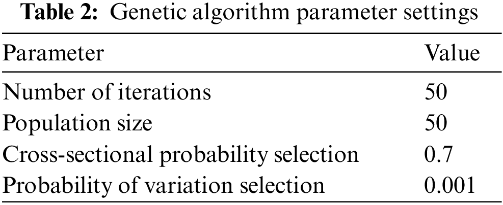
The parameters of GA are initialized as shown in Table 2.

3.4 Experimental Program

Simulation of Urban Mobility (SUMO) is a microscopic, multimodal traffic simulation developed by the German Aerospace Center, an open-source traffic simulation software that can visually study the changing characteristics of a vehicle or traffic flow and can better simulate the movement process of vehicles, including the length and width of vehicles, the acceleration, and deceleration process of vehicles, and the interaction between vehicles. It is therefore widely used by scholars who study traffic simulation. This paper builds a simulation model based on SUMO software and uses the control variable method to investigate the relationship between the capacity of junctions and factors such as vehicle speed, acceleration, green letter ratio, and widened lane length respectively to provide a corresponding theoretical basis for the improvement of junctions in real life.

Our experimental scenario is shown in Fig. 1. According to the actual intersection physical conditions including phase situation, lane number situation, right-turn green light situation, the actual signal timing situation, and the actual traffic flow, and the different starting acceleration habits of the drivers, the Webster algorithm and the multi-objective GA optimization are respectively imported. The average junction delay, junction capacity, junction stopping times, and junction signal periods of the two algorithms are obtained and compared, and the conclusion is that the GA-based multi-objective optimization timing scheme performs significantly better than the Webster timing scheme. The existing timing scheme, the Webster timing scheme, and the GA-based multi-objective optimized timing scheme are then imported into the SUMO simulation model for experimental validation. Using the vehicle travel information from the SUMO simulation experiment, different timing schemes were obtained in terms of total lost time, CO emissions, PM emissions from solid particulate matter, and vehicle fuel consumption, and conclusions were drawn from these comparisons.

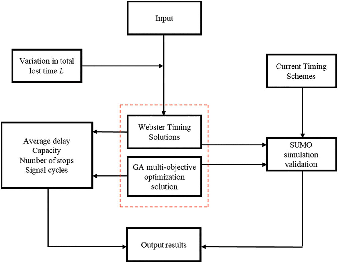
Figure 1: Experimental flow chart

4  Case Study

4.1 Experimental Area and Dataset

We selected the intersection of Huaishun Middle Road and Dongshan East Road in Tianjia’an District of Huainan City, Anhui Province, China. Huaishun Middle Road is the second major north-south road that runs through the old and new urban areas of Huainan City and connects directly to Huainan High-Speed Railway South Station to the south. Crossing the railway to the north, it enters the main urban area. The intersection leads east to the Datong district of Huainan City and west to Dongshan Middle Road and Dongshan West Road, which lead to several other counties in the city. Due to the particularity of this intersection, the intersection is 400 m to the north (needing to cross the railway), and it is a three-way intersection leading to the old city, and the road widening in this direction is limited. At the same time, the traffic flow of people and vehicles at the intersection is very heavy, especially during the morning and evening rush hours, and congestion often occurs. It is planned to first model and optimize a single intersection and then model and optimize two neighboring junctions.

The following assumptions are made: (1) Ignore the effect of right-turning traffic on the capacity of the intersection. (2) Ignore the effect of pedestrians and non-motorized vehicles on the intersection capacity. (3) Ignore the effect of primary and secondary roads at the intersection. (4) Ignore the railroad underpass structure in the northern section of the intersection.

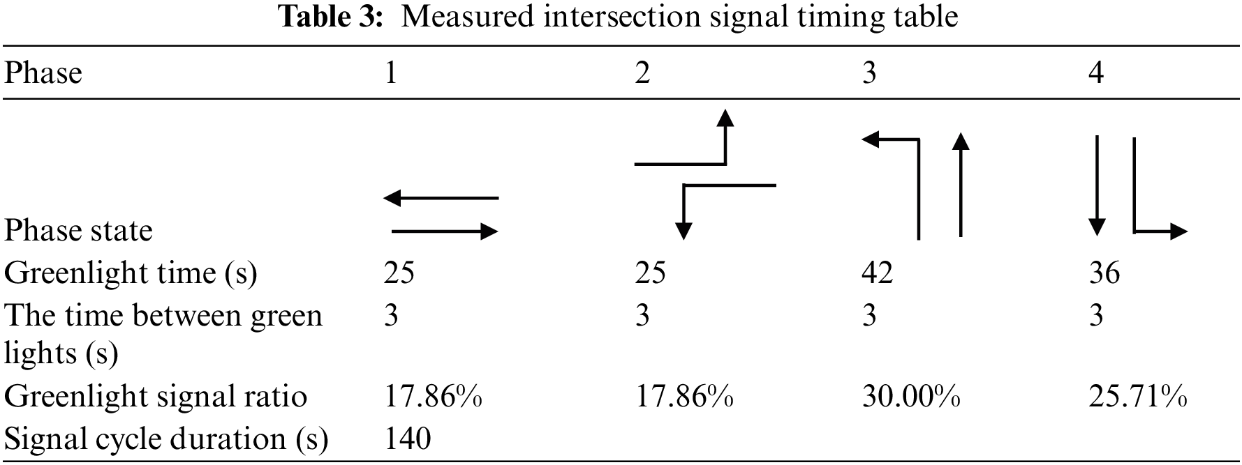
Since the four directions of this intersection are right-turn green, the impact of right-turn vehicles on this intersection can be ignored as long as the traffic rules are observed. The intersection signal timing table is shown in Table 3. Which indicates that there are four phases at the intersection. Specifically, the first phase is east or west. The second phase is the east left turn, and west left turn. The third phase is the south left turn, south straight ahead. The fourth phase is a north left turn, north straight ahead; the signal cycle of the intersection is 140 s, the yellow time is 3 s, and there is no all-red time. The green time for phase 1 is 25 s with a green signal ratio of 17.86%, phase 2 has a green time of 25 s with a green signal ratio of 17.86%, phase 3 has a green time of 42 s with a green signal ratio of 30.00% and phase 4 has a green time of 36 s with a green signal ratio of 25.71%.

The measured data for this junction is the actual junction traffic information during the evening peak hours of 17:30 to 18:30 on September 7, 2022. The measured data for each direction of traffic flow, lane information, traffic flow information, and traffic volume information when ignoring right-turning traffic at the intersection are shown in Table 4.

Since the following assumptions were made in this paper: ignoring while ignoring the effect of right-turning vehicles at junctions on intersection capacity, ignoring the effect of pedestrians and non-motorized vehicles on intersection capacity, and ignoring the effect of primary and secondary roads at junctions, data related to assumptions are not recorded in Table 4.

4.2 Experimental Performance Comparison of Various Algorithms

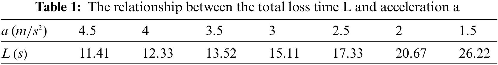
The junction conditions and road speed limit are fixed. The braking loss time and the road speed limit are set to 1 s and 60 km/h, respectively. Considering the different starting acceleration habits of drivers, we set starting acceleration as 1.5, 2, 2.5, 3, 3.5, 4, and 4.5 m/s2 variables to observe the effect of changes in starting acceleration on starting loss time. Meanwhile, the average delay, total capacity, number of stops, and signal period were calculated by using the Webster algorithm and the multi-objective GA, respectively. The results of junction delays between Webster and multi-objective GA are shown in Table 5 and Fig. 2.

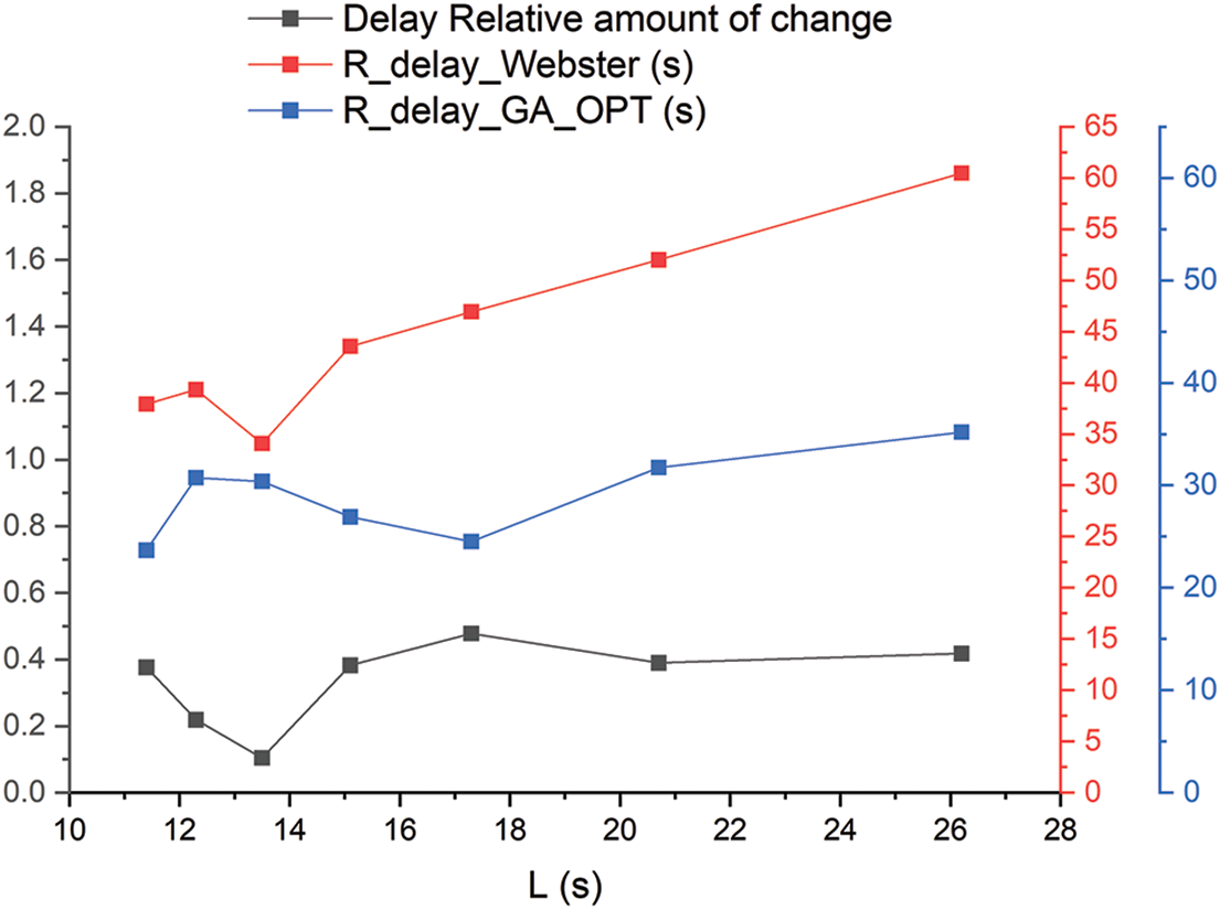
Figure 2: Comparison of average delay between Webster and multi-objective GA

As shown in Table 5 and Fig. 2, when the driver’s starting acceleration gradually decreases and the total loss time L gradually increases, the average delay in junction obtained by the Webster algorithm timing scheme increases significantly, while the average delay in junction obtained by multi-objective GA becomes larger, and the effect is better than Webster algorithm. In summary, in the multi-objective GA compared to the Webster algorithm, the maximum delay in junction is 47% reduction, the minimum delay in junction is 10.5% reduction, and the average delay in junction is 34.8% reduction.

The impact of the Webster algorithm and multi-objective GA timing results on junction capacity is shown in Table 6 and Fig. 3.

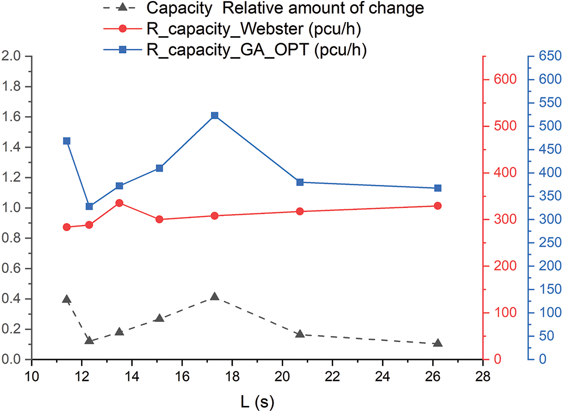
Figure 3: Comparison of junction capacity between Webster and multi-objective GA

As shown in Table 6 and Fig. 3, when the driver’s start acceleration gradually decreases and the total loss time L gradually increases, the junction capacity obtained by the Webster algorithm timing scheme does not change much, while the junction capacity obtained by the multi-objective GA becomes larger, and the effect is better than Webster algorithm. In summary, in the multi-objective GA compared to the Webster algorithm, the maximum capacity in junction capacity is a 41% increase, the minimum capacity in junction capacity is a 10.4% increase, and the average capacity is a 25.2% increase.

The impact of the Webster algorithm and multi-objective GA timing results on the number of intersection stops is shown in Table 7 and Fig. 4.

Figure 4: Comparison of the junction stops between Webster and multi-objective GA

As shown in Table 7 and Fig. 4, when the driver starts acceleration gradually decreases and the total loss time L increases, the number of junction stops obtained by the Webster algorithm timing scheme does not change much, while the number of junctions stops obtained by the multi-objective GA becomes fewer, and the effect is slightly better than Webster algorithm. In summary, in the multi-objective GA compared to the Webster algorithm, the maximum number of stops is 14.4% reduction, the minimum number of stops is 2.6% reduction, and the average number of stops is 6.45% reduction.

The impact of the Webster algorithm and the multi-objective GA timing results on the traffic signal cycle is shown in Table 8 and Fig. 5.

Figure 5: Comparison of cycle between Webster’s algorithm and multi-objective GA

As shown in Table 8 and Fig. 5, when the driver’s start acceleration gradually decreases and the total loss time L gradually increases, the junction signal cycle obtained by the Webster algorithm timing scheme changes faster, while the junction signal cycle obtained by the multi-objective GA changes more slowly, and the effect is better than Webster algorithm. In summary, in the multi-objective GA compared to the Webster algorithm, the maximum Cycle is 42.8% reduction, the minimum Cycle is 2.8% reduction, and the average Cycle is 22.8% reduction.

4.3 Simulation Verification

Our SUMO simulation model is based on the Krauss model of vehicle motion [25] and uses the following five parameters.

a: Maximum acceleration during vehicle acceleration (m/s2).

b: Maximum acceleration during the braking phase of the vehicle, with b being a negative value (m/s2).

Vmax: The maximum speed allowed for the vehicle to travel (km/h).

l: Vehicle length (m).

KDP: The driver’s driving proficiency, a smaller value indicates a more proficient driver.

The model uses Eq. (21) in the calculation of safe vehicle speeds.

Vsafe=VB(t)+g(t)−VB(t)TDR(VB(t)+v(t))2b+TDR(21)

where VB(t) is the speed before the moment t, v(t) is the speed of that car at the moment t, g(t) is the shop distance between the car in front and behind at the moment t and TDR is the driver’s reaction time.

In SUMO simulation software, we use Eq. (22) to complete this model experiment.

vs=−TDR∗b+(TDR∗b)2+VB2+2b∗g(t)(22)

4.4 Intersection Simulation

In this simulation experiment, the version of SUMO is sumo-win64-1.14.0. A 5 * 5 road network model was constructed in SUMO’s own Netedit road network editing software. Specifically, the distance between nodes was 1000 m. According to the parameters of the actual intersection, the road network model of the actual intersection is constructed in the road network model. In the vehicle simulation parameter settings, the maximum acceleration of the vehicle when accelerating is a = 2.5 m/s2, the maximum acceleration of the vehicle when braking is b = −4.5 m/s2, the maximum speed allowed for the vehicle is Vmax = 16.67 m/s2, the body length: l = 5 m, and the driver’s driving proficiency: KDP = 0.5.

The field survey data and the optimized timing scheme were input into each module of the SUMO simulation software. The SUMO simulation process was based on the existing geometric characteristics, signal timing scheme, and measured traffic demand values of the intersection of Dongshan Road and Huaishun Avenue North, and the simulation program was established, and the simulation results are shown in Fig. 6.

Figure 6: SUMO simulation of an actual intersection

4.5 Analysis and Comparison of Simulation Results

To compare the effect of the timing scheme before and after optimization, average lost time, average carbon monoxide (CO) emissions, average particulate matter (PM) emissions of particulate matter, and average fuel consumption were selected as evaluation indicators to be presented in Table 9.

According to the experimental results of the SUMO simulation model in Table 9, the average loss time is 33.11 s after applying the Webster algorithm, which is 11.59% shorter than the status quo. The average CO emission is 6480 g, which is 10.10% less than the status quo. The average PM emission is 6.9 g, which is 3.9% less than the status quo. The average fuel consumption is 171.26 ml, which is 2.62% less than the status quo. The average fuel consumption is 171.26 ml, which is 2.62% lower than the status quo.

From Table 9, we can also get that the average loss time of GA multi-objective optimization is 32.42 s, which is 13.46% shorter than the status quo and 2.11% shorter than Webster’s algorithm; the average CO emission of GA multi-objective optimization is 6402 g, which is 11.18% shorter than the status quo and 1.2% shorter than Webster’s algorithm. The average PM emission of particulate matter is 6.89 g, which is 4.04% less than the status quo and 0.14% less than the Webster algorithm. The average fuel consumption of GA multi-objective optimization is 171 ml, which is 2.77% less than the status quo and 0.15% less than the Webster algorithm.

Therefore, from Table 9, the following conclusions can be drawn: (1) The simulation results of both the Webster algorithm and the GA multi-objective optimization are better than the pre-optimization solution. (2) The GA multi-objective optimization based on the Webster algorithm is slightly better than the Webster algorithm.

5  Conclusion

Since the conclusions in this paper were obtained while ignoring the effect of right-turning vehicles at junctions on intersection capacity, ignoring the effect of pedestrians and non-motorized vehicles on intersection capacity, and ignoring the effect of primary and secondary roads at junctions, the conclusions obtained were somewhat limited.

In this paper, taking the shortest average delay time, the least average stops, and the maximum capacity of the intersection as the objective function of our GA multi-objective optimization, a nonlinear multi-objective optimization model of urban intersection signal timing based on our GA multi-objective optimization is constructed. The study results show that our GA multi-objective optimization is significantly superior to the Webster algorithm in optimization variables of average junction delay time, junction capacity, number of junction stops, and signal cycle duration. The correctness of our GA multi-objective optimization algorithm was verified at SUMO. The simulation results show that our GA multi-objective optimization is the best, Webster is the second best, and the pre-optimization solution is the worst in performance metrics including the average lost time, average CO emission, average particulate PM emission, and average fuel consumption.

Funding Statement: The research is supported by the joint NNSF&FDCT Project Number (0066/2019/AFJ) and joint MOST&FDCT Project Number (0058/2019/AMJ), City University of Macau, Macao, China.

Conflicts of Interest: The authors declare that they have no conflicts of interest to report regarding the present study.

References

1. S. Jafari, Z. Shahbazi and Y. C. Byun, “Designing the controller-based urban traffic evaluation and prediction using model predictive approach,” Applied Sciences, vol. 12, no. 4, pp. 1992, 2022. [Google Scholar]

2. W. Heng, L. M. Han, W. Z. Yu, L. Wei, H. T. Jiao et al., “Heterogeneous fleets for green vehicle routing problem with traffic restrictions,” IEEE Transactions on Intelligent Transportation Systems, pp. 1–10, 2022. https://doi.org/10.1109/TITS.2022.3197424 [Google Scholar] [CrossRef]

3. C. G. Tang, S. X. Xia, C. S. Zhu and X. L. Wei, “Phase timing optimization for smart traffic control based on fog computing,” IEEE Access, vol. 7, pp. 84217–84228, 2019. [Google Scholar]

4. W. B. Kou, X. M. Chen, L. Yu and H. B. Gong, “Multiobjective optimization model of intersection signal timing considering emissions based on field data: A case study of Beijing,” Air & Waste Management Association, vol. 68, no. 8, pp. 836–848, 2018. [Google Scholar]

5. F. Webster, “Traffic signal settings,” Road Research Laboratory, London, U.K, Road Res. Tech. Paper 39, 1958. [Google Scholar]

6. R. Akcelik, “Capacity and timing analysis,” Research Report ARR, Victoria, Australia, no. 123, 1981. [Google Scholar]

7. Q. Lu and K. D. Kim, “A genetic algorithm approach for expedited crossing of emergency vehicles in connected and autonomous intersection traffic,” Journal of Advanced Transportation, vol. 2017, pp. 1–14, 2017. [Google Scholar]

8. R. Guo and Y. Zhang, “Exploration of correlation between environmental factors and mobility at signalized junctions,” Transportation Research Part D: Transport and Environment, vol. 32, pp. 24–34, 2014. [Google Scholar]

9. W. Peng, “Research on vehicle routing optimization problem of urban real-time traffic road network,” Journal of Vehicle and Intelligent Transport System, vol. 1, no. 1, pp. 1–5, 2019. [Google Scholar]

10. H. Mohapatra, A. K. Rath and N. Panda, “IoT infrastructure for the accident avoidance: An approach of smart transportation,” International Journal of Information Technology, vol. 14, no. 2, pp. 761–768, 2022. [Google Scholar]

11. R. Montemanni, L. M. Gambardelia, A. E. Rizzoli and A. V. Donati, “Ant colony system for a dynamic vehicle routing problem,” Journal of Combinatorial Optimization, vol. 10, no. 12, pp. 327–342, 2005. [Google Scholar]

12. H. Mohapatra and A. K. Rath, “An IoT-based efficient multi-objective real-time smart parking system,” International Journal of Sensor Networks, vol. 37, no. 4, pp. 219–232, 2021. [Google Scholar]

13. K. Fang, T. Wang, X. Zhou, Y. Ren, H. Guo et al., “A TOPSIS-based relocalization algorithm in wireless sensor networks,” IEEE Transactions on Industrial Informatics, vol. 18, no. 2, pp. 1322–1332, 2022. [Google Scholar]

14. J. P. Rojas Suárez, M. S. Orjuela Abril and G. C. Prada Botia, “Diagnosis of road capacity and service level using the highway capacity manual,” Journal of Physics, vol. 1674, no. 1, pp. 12–19, 2020. [Google Scholar]

15. I. A. Aljabry and G. A. AI-Suhail, “A survey on network simulators for vehicular ad-hoc networks (VANETS),” International Journal of Computer Applications, vol. 174, no. 11, pp. 1–9, 2021. [Google Scholar]

16. A. Tamini, M. AbuNaser, A. A. Tavalbeh and K. Saleh, “Intelligent traffic light based on genetic algorithm,” in Proc. JEEIT, Amman, Am, Jordan, pp. 851–854, 2019. [Google Scholar]

17. D. Thomas and B. C. Kovoor, “A genetic algorithm approach to autonomous smart vehicle parking system,” in Proc. ICSCC, Kurukshetra, India, pp. 68–76, 2018. [Google Scholar]

18. A. M. Turky, M. S. Almad and M. Z. M. Yusoff, “The use of genetic algorithm for traffic light and pedestrian crossing control,” International Journal of Computer Science and Network Security, vol. 9, no. 2, pp. 88–96, 2009. [Google Scholar]

19. C. P. Pappis and E. H. Mamdani, “A fuzzy logic controller for a traffic junction,” IEEE Transactions on Systems, vol. 7, no. 10, pp. 707–717, 1977. [Google Scholar]

20. D. X. Cheng, C. J. Messer, Z. Z. Tian and J. Y. Liu, “Modification of Webster’s minimum delay cycle length equation based on HCM 2000,” in Proc. TRB, Washington, D. C, USA, 2003. [Google Scholar]

21. Q. P. Wang, X. L. Tan and S. R. Zhang, “Signal timing optimization of urban single-point intersections,” Journal of Traffic and Transportation Engineering, vol. 6, no. 2, pp. 60–64, 2006. [Google Scholar]

22. Y. Jin and R. H. Yao, “Optimization models of pretimed signal timing for isolated intersections,” Journal of Dalian Jiaotong University, vol. 32, no. 6, pp. 30–35, 2011. [Google Scholar]

23. J. H. Holland, “Genetic algorithms,” Scientific American, vol. 267, no. 1, pp. 66–73, 1992. [Google Scholar]

24. F. F. Mu and H. Z. Zhang, “Signal timing optimization at single-point intersection based on genetic algorithm,” University of Shanghai for Science and Technology, vol. 37, no. 6, pp. 600–604, 2015. [Google Scholar]

25. V. Kanagaraj, G. Aaaithambi, C. H. Naveen Kumar, K. K. Srinivasan and R. Sivanandan, “Evaluation of different vehicle following models under mixed traffic conditions,” in Proc. CTRG, Agra, India, pp. 390–401, 2013. [Google Scholar]