Improvements in Weather Forecasting Technique Using Cognitive Internet of Things

1  Introduction

One can do weather forecasts for a specific location and time based on different environmental conditions. The most challenging aspect of predicting the weather is figuring out how to deal with uncertain and contradictory situations. Precise predictions can be made using the maximum number of real-time feasible weather-affecting predictors for accounting for weather conditions. Cognitive computing (CC) assists us in analyzing situations like these. As weather conditions change frequently, our model may not make a clear decision. Cognitive Computing (CC) is helpful at that point because it works the same way as a human brain. The goal of the model ought to be adjusted on an ongoing basis to concentrate on reaching the objective. One can accomplish this by considering all perspectives and will make decisions based on the optimal adjustment of the weight of the inputs rather than concentrating on the precise output. In every way imaginable, the operation of cognitive computing is analogous to that of the human brain. As the human brain draws its past experiences and logical deliberation to make choices when faced with competing options, our model in CC will always be ready to figure out a perfect solution rather than clinging to a rigid move when faced with unfamiliar circumstances [1].

The forecasting activity bears a great deal of significance because it uses both technical tools and scientific methods. Even though many forecasting systems are, and many produce accurate result, none can guarantee that there will be no fatigue in the future. The Authors utilized various sensors for data collection and training on previously collected data. The Authors make predictions using predictors, i.e., temperature, pollution, humidity, wind direction, precipitation, and pressure. Suppose people want to calculate the damage in the form of numbers. In that case, they can collect data from the metrological department for a specific location and then conduct a regression analysis. It will allow visualizing a numerical estimate of the damage. Before beginning the prediction process, data should be normalized and scaled to eliminate redundancy and ensure one can generate an optimized view. People should collect data using cognitive sensing to ensure the process is as efficient as possible. Because the data collected by Internet of Things devices will be real-time and of varying sizes, the Authors have used methods such as data aggregation, fusion, remote data collection, and so on to make the data collection process intelligent [2]. The present study will be essential in many fields, i.e., tourism, farming, transportation, etc. Individuals can mitigate possible disruptions using the Cognitive Internet of things (CIoT) Setup.

2  Related Works

Reference [3], A decision tree-based model was presented based on a data mining approach. Metrological data used by the Authors are from four years, 2012 to 2015, of different cities. The initial data was pre-processed to make it suitable for data mining. The decision tree contains two parameters, i.e., Maximum temperature and minimum temperature. The Authors found a temperature greater than 35 mm means it will indicate full hot, and if the temperature is <=30, it will simply indicate hot. If the temperature <25, it will be counted as the minimum temperature, and if the temperature value <=10, it will be cold. The Authors explain how this temperature parameter affects the weather. Still, the drawback is this it is only one parameter that can’t be used for exact prediction as weather includes many permanents. In the paper [4], a data mining algorithm for weather forecasting was implemented. The model used for prediction is a Hidden Markov Model (HMM), and the K-means clustering algorithm extracts appropriate data about weather conditions. The Authors have used Bhopal weather data for five years for training and testing. Similar kinds of attributes are combined using K-means clustering. The data generated by this algorithm is provided to the HMM, and Authors get their prediction output. The Authors have also compared traditional methods regarding the time taken in training and prediction. Here the Authors found some limitations as to when training data increases, training time also increases. According to [5], a statics-based weather prediction model was built using fuzzy logic. Data from Northeastern Thailand were used to predict input parameters such as solar radiation, temperature, wind speed, and humidity. All input is taken into account by fuzzification using the membership function. The parameters used in the fuzzification rule for 5 min of past data are: Very High, High, Medium, Very Low, Low, and at the last, defuzzification process to predict the rainfall. A comparison was made with the static model prediction error and Root Mean Square Error. The Authors found that the model fuzzy model is more reliable and efficient than the static model.

The Authors have surveyed different neural network techniques used in the past 20 to 30 years for prediction [6]. It has been concluded that most of the Authors have used the BPN network for prediction. Backpropagation neural networks yield a better result than the past metrological approaches for prediction as they can handle the non-linear relationship between the past data. In the end, it has been said that for a more accurate forecast, there should be maximum training data and many parameters. Various activities that define the use of computer-assisted mental processes (cognitive computing) in realistic environments have been discussed [7]. The computer of the mind found the growth of self-aware programs that interact automatically with people in complex and adaptable contexts and changes in language and results. These programs mimic the human mind’s processes, define an extensive range of data, find correlations, evaluate theoretical ideas, make predictions and indicators, draw conclusions, and so on. A model is implemented that has a nature to augment algorithmic rule that gives approximate or nearby results for forecasting of upcoming five days and at the last outcomes is calculated with a crisp and statistical decision tree and prepare a confusion matrix for forecasting using Big Data [8]. The Authors have predicted rainfall and temperature using four different algorithms based on different error parameters and concluded that among several machine learning algorithms, for rainfall prediction multi-Layer perceptron (MLP) is the best and for temperature prediction best model is Support vector Regression [9]. The Authors reviewed IoT data features and their difficulties with Deep Learning (DL) methods [10]. They also introduced a few fundamental DL structures used to reference IoT modules. Analyzing various models in the many IoT applications using DL has been included in this study in which the Authors explore five primary resources and eleven application domains. The Authors created a solid background for future researchers in understating the core idea of IoT smart devices and also gave an insight into the challenges and a guided path for DL in IoT Models. A forecasting system with low-cost sensors has been presented by the Authors [11]. The core predictors are temperature, light, and humidity. Data is loaded in the thing speak cloud. The model is trained with past recorded values and is used to predict future values. The last prediction results are compared with other models and found that this gives little more accuracy than the others. In the paper [12], the Authors reviewed the technology used for the implementation of automated weather stations is being made. In addition, the Authors also introduced the advanced computing such as IoT, Edge Computing, In-Depth Learning, Low Power WAN (LPWAN), etc. using upcoming AWS-based viewing systems. In the paper [13], the Authors presented a data-driven model based on long short-term memory modes (LSTM) and convolutional short-term networks (TCN) and analyzed the performance with current machine learning methods. In the LSTM model, the Authors find two states, a hidden state that measures short-term memory and a self-state holding long-term memory that deals with long sequences. The Authors conclude that their lightweight way is more accurate than famous weather research and forecasting (WRF) models. In the paper [14], the Authors introduced a system for actual-time weather conditions and forecasting in a real-time bus management system having four key components i.e., Data management, an information-rich bus stop, a future decision model, and a website to display all.

The potential and challenges of AI strategies for cognitive sensory (CS) solutions to future Internet of Things (FIoT) models have been explored [15]. In FIoT, useful actions generated from AI algorithms will be implemented by IoT devices. The Cognitive Sensing method will be applied to IoT (FIoT) framework to simplify the intelligent data-gaining process. Four methods in cognitive sensing i.e., efficient power consumption, auto-heal management, security, and smart data collection are briefly discussed. In the paper [16], the Author has developed a model based on 11 months of previously recorded data on rainfall, temperature, and humidity to predict groundwater levels. Three machine learning algorithms have been applied for prediction i.e., Extreme Gradient Boosting (XGBoost), Artificial Neural Network (ANN), and Support Vector Regression. A detailed review has been done of current research activities involved in weather forecasting and compared their results [17]. An analysis mainly using predictors as an input and weather conditions as a target variable has been done. A conclusion is made that there is a lack of stability in current weather forecasting systems. In the paper [18], the Authors illustrated that the convolutional neural network, which is more widely used in processing satellite images than the statistical climate figures for temperature prediction, surpasses other algorithms. The Authors prepared a global model for weather forecasting using machine learning [19]. A model is prepared to keep in mind the compatible design of modern computers. The model’s accuracy is compared with daily climate, persistence, and numerical models facing the same kind of variance. The framework predict real-world weather fluctuations for all global forecast periods. The ML model surpasses weather science and persistence in the forecast in the central, but not in the tropics. Compared to the numerical model, the ML model works much better with the status variables that are much influenced by the parameter deployed in the numerical model. A comparison of the accuracy of the two rain forecast models based on LSTM and advanced machine learning algorithms has been done [20]. To obtain this goal, 2 LSTM-Networks-based models, 3 Stacked-LSTM-based models, and Bidirectional-LSTM Networks model were compared to XGBoost (the basic model) and the integrated model developed for Learning Default Machine. In the paper [21], a model is prepared aiming at low cost as a central feature for monitoring weather conditions. In the model, various sensors have been used for detecting environmental data. The primary aim is to make the system more affordable so everyone can use it freely. In the paper [22], multi-class weather classification using autonomous IoT has been done. A prediction scheme for cumulative electricity consumption using time series data has been implemented [23]. The Authors have created a deep learning-based framework to categorize weather conditions for an autonomous vehicle [24].

3  Material and Methods

3.1 IoT Sensors and Dataset Collection

In the Internet of things, a network is established to send the data across the internet with the help of sensors. It helps humans to control the associated devices from anywhere. Early identification of the unusual pattern from the assigned device prevents future heavy damage.

First, the Authors collected data from Kaggle and refined it using the normalization process. The dataset provides data from 1st May 2016 to 11th March 2018. It gives a list of parameters: Mean temperature, Mean dewpoint, Mean pressure, Max humidity, Min humidity, Max temp, Min temp, Max dewpoint, Min dewpoint, Max pressure, Min pressure, etc.

Then, the Authors collected real-time weather data using different IoT sensors i.e., DHT11 for measuring temperature and humidity, BMP 180 for measuring biometric pressure, rain sensor for measuring the amount of rainfall, anemometer to measure wind speed, and wind wave sensor for wind direction. The Authors have also used a dataset that contains 21 years of daily weather observations across the Lucknow Region [25].

3.2 System Requirements

An online platform called the Arduino IoT Cloud makes it simple to design, implement, and keep track of IoT networks. The Authors draught Arduino IDE (Integrated Development Environment) to code Arduino, and for executing all machine learning algorithms, they used Jupyter Lab.

3.3 Methodology

Meanwhile, reviewing many previous works, the Authors have decided to build a model based on weather-affecting paraments pressure, humidity, rainfall, temperature, dust, light, etc., to predict the weather conditions. The ensemble model can predict the next day’s rain using previous data. Existing weather forecasting models have many statistics and use satellite data but are not correctly designed to accurately reflect local climatic data. As climate data changes randomly from one location to another, one cannot entirely rely on satellite-based monitoring.

Many previous models were acknowledged for collecting weather information, and the Authors’ primary aim was to improve results at a low cost. The Authors have changed previous strategies and keep focusing on the best approaches for weather forecasting-related activities. They entail a computer language for implementing our machine-learning code. The Authors chose Python as a language due to its information-rich library so that we easily store and process our data. The Authors use the Anaconda Software package, and all training and testing have been done in Jupyter.

In this paper, the Authors have used the Decision Tree algorithm (DT), Logistic Regression (LR), Support Vector Machine (SVM), Neural Network (NN), Random Forest Classifier, and extreme gradient boosting XGBoost algorithm for rainfall prediction.

3.3.1 Decision Tree Algorithm

The Decision Tree Algorithm mainly comes under supervised learning. In this, the Authors first go for the Root selection of the tree. Then they compare the root with the recorded attribute. Based on the comparison, the Authors decide which branch to follow based on the inclusion or exclusion of outcomes [26].

3.3.2 Logistic Regression

A supervised learning method is used to monitor this as well. It predicts phase-based fluctuations using a given set of independent variables. Stress indicates the outflow of phase-dependent variability. Therefore, the result must be a different category or value. Either Yes or No, 0 or 1, True or False, etc. but instead of giving a direct value such as 0 and 1, it provides possible values between 0 and 1 [27].

3.3.3 Support Vector Machine

Support Vector Machine (SVM) is a machine-readable learning algorithm that can be used for classification and regression problems. If we have sample data on which each data point belongs to one of two categories, SVM produces a model that assigns new data to one category or another. It works as a non-probabilistic binary linear classifier. We use a hyperplane that separates the categories [28].

3.3.4 Neural Network

A neural network is a sequence of actions used to find the correlation among a data set in the same way a human brain works. We adjust the weights of the inputs without restarting the output state. It works in the same way the neuron system works in the human brain. It uses experience and classifies the data [29].

3.3.5 Random Forest

It is an ensemble learning way for classification and regression tasks. It consists of many decision trees. Every tree in the random forest votes out for a class prediction, and the class that gets the maximum votes will act as a final prediction by the model. As a group of trees, our forecast moves in the right direction [30].

3.3.6 XGBoost

XGBoost uses advanced decision-making trees designed for speed and performance, a highly competitive learning machine. XGBoost represents Extreme Gradient Boosting, which was proposed by researchers at the University of Washington. It is a C ++ written library that enhances the Gradient Boosting training [31].

4  Proposed System

Once our goal becomes clear, the Authors build a model that collects data from different sensors. Sensors give an idea to carry some specific processes in a particular time range, i.e., the humidity sensor specifies when fertilization is needed for a particular crop. The data is collected from sensors on daily bases for the duration of the past 365 days in the Lucknow (U.P) region. The main parameters considered are Temperature (C), Humidity (%), Atmospheric pressure (hPa), Wind direction (degree), Wind speed (m/s), and Rainfall (mm). The Authors have used binary classification and a multiclass model to classify light, moderate and heavy rain.

Several Machine learning algorithms have been applied in this paper, and result analysis has been done using a Confusion matrix, precession, and finally compare their accuracy to find the best fitting algorithm. The Authors also have used the weather Australia Dataset for the past twenty years that they get from Kaggle to compare the performance with sensor data. The Authors did data analysis and identified relevant parameters. Meanwhile, the Authors used ensemble modelling to conduct the following research. The Authors used a stacking method that trains different machine learning algorithms, i.e., Support Vector Machine, Random Forest Classifier, ANN, Logistic Regression, Decision Tree, and XGBoost Algorithms and combines all the learners to improve the prediction power. Use Fig. 1.

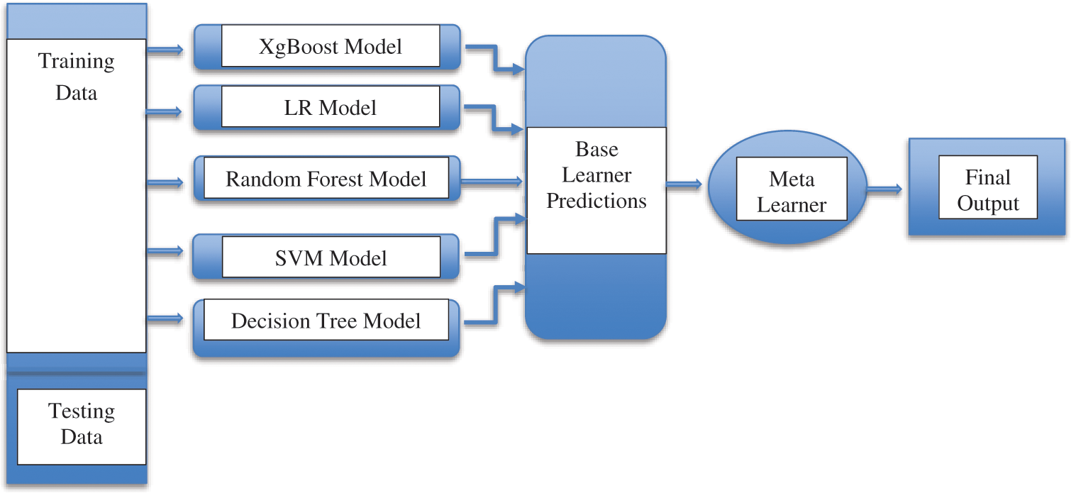
Figure 1: Architecture of proposed method

Authors have used Stacked Model for combining the different machine learning algorithms. It entails integrating the predictions from various machine learning models on a single data set. See Fig. 5.

4.1 Training Set Description

The Authors trained this model on the past 20 years of Australian weather data and were able to predict the next day it would rain or not (classification problem). The Dataset Column “Rain Tomorrow” was chosen as a dependent variable over other columns as the independent variables. The dataset for training and testing was divided using the train_test_split () function; the test size that the Authors kept was 20%.

4.2 Correlation Plot

The Authors selected only those predictors showing a high correlation in the study. In the graph, as the max temperature increases, the min temperature increases, so the probability of rain tomorrow increases. See Fig. 2.

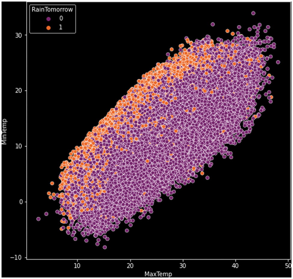
Figure 2: Correlation matric (min temperature and max temperature for next-day rainfall) (x-axis: maximum temperature variable, y-axis: minimum temperature variable)

Now in the graph, as humidity increases, the temperature increases, so the probability of rain tomorrow increases (see Fig. 3).

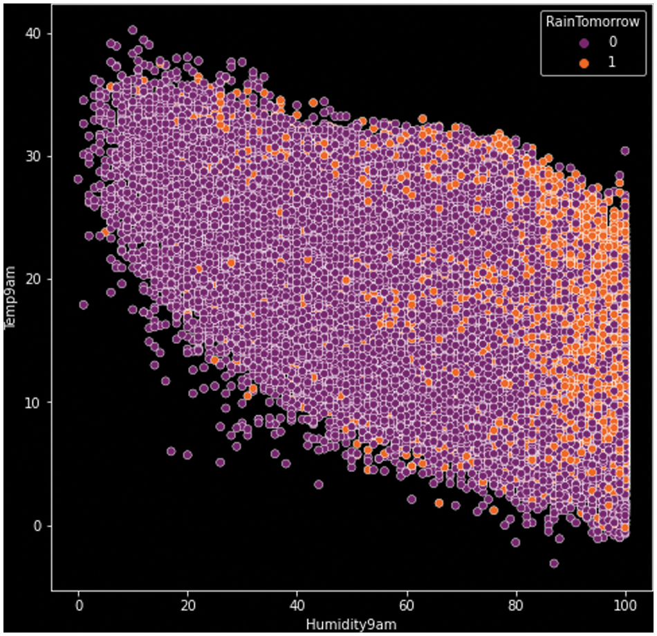
Figure 3: Correlation matric (humidity at 9 am and temperature at 9 pm for next-day rainfall) (x-axis: humidity at 9 am variable, y-axis: temperature at 9 pm variable)

4.3 Heatmap

It shows a correlation between each data frame column to the rain tomorrow column; the lighter the colour, the better the relationship. See Fig. 4.

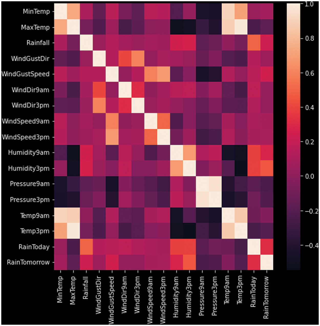
Figure 4: Heatmap (correlation between each and every column) (x-axis: category on the horizontal scale, y-axis: category on the vertical scale of daily observations)

5  Performance Measure

Our XGBoost model may suffer from high variance; the Authors avoid it by keeping less difference in training and test data. To evaluate the performance and comparative analysis of various computational intelligence techniques, it is necessary to calculate the multiple parameters involved in the Performance Measure. There are various parameters involved in the performance measure. Some of them are as follows:

Accuracy: In the accuracy formula numerator contains True Positive and True Negative, and the denominator, contains all the predictions made by the model. It is crucial in the classification problem and defines as the ratio of the number of correct predictions made by the model over the total prediction made [32].

It is calculated mathematically as follows:

Accuracy=TP+TNTP+FP+FN+TN(1)

Precision: It is a measure that describes the ratio of true positive and summation of positive predictions made by the model.

It is calculated mathematically as follows:

Precision=TPTP+FP(2)

Recall: It is also called Sensitivity. It is a measure that describes the ratio of True Positive for all positive data points.

It is calculated mathematically as follows:

Recall=TPTP+FN(3)

Specificity: It is exactly the opposite of Recall. It is a measure that describes the proportion of True Negative for all negative data points.

It is calculated mathematically as follows:

Specificity=TNTN+FP(4)

F-Measure: It is also called the F-Score. It is the Harmonic mean of Precision and Recall. It is denoted by F.

F=2∗Precision∗RecallPrecision+Recall(5)

5.1 Model Stacking

It is a machine learning ensemble technique that combines several machine learning algorithms into a principal learner using a baseline classifier. First, each algorithm will make its prediction. Then, prediction probability will be used as input for the meta-learner to combine the algorithms’ predictive performance. The Meta-model discovers the optimal way to integrate the prediction capability of base models.

6  Results and Discussion

The Authors compare different machine learning algorithms and found that XGBoost has the highest accuracy among the entire model. It performs better on all the chosen datasets. The XGBoost-based approach achieved an accuracy of 86%, Precision values of 85%, Recall values of 86%, and F1-score of 85%, using Australian rainfall data Table 1. Bold values show the outcome of the ensemble method.

The XGBoost-based approach also achieved accuracy of 99.25% Precision values of 99% Recall values of 99% and F1-score of 99% using sensor data Table 2. Bold values show the results of the ensemble method.

6.1 Learning Rate of the Proposed Algorithm

The nature of the XGBoost algorithm is that they are fast in learning which may lead to overfitting. This can be avoided by the shrinkage factor (slowing the learning). In Fig. 6, the X-axis shows the number of iterations, and the y-axis shows the log loss of the model.

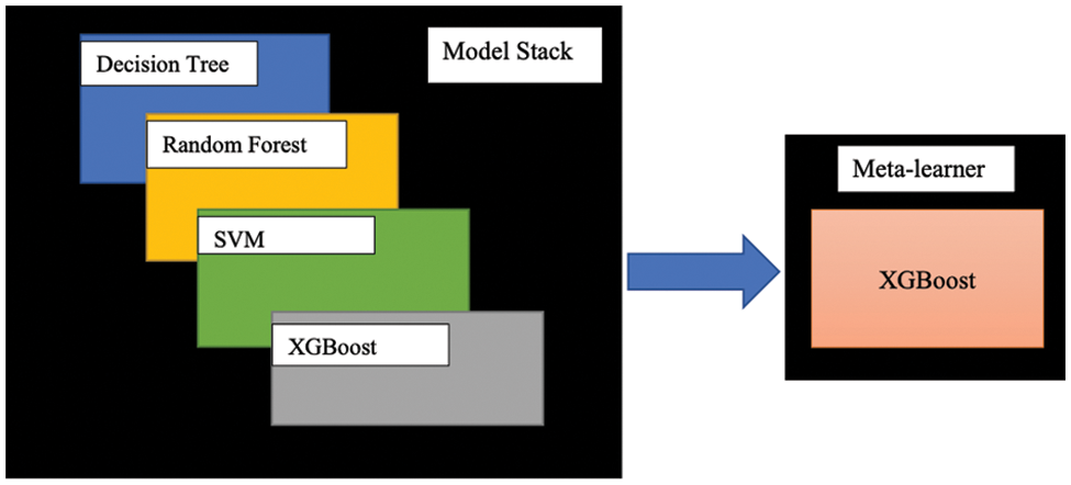
Figure 5: Stacked model

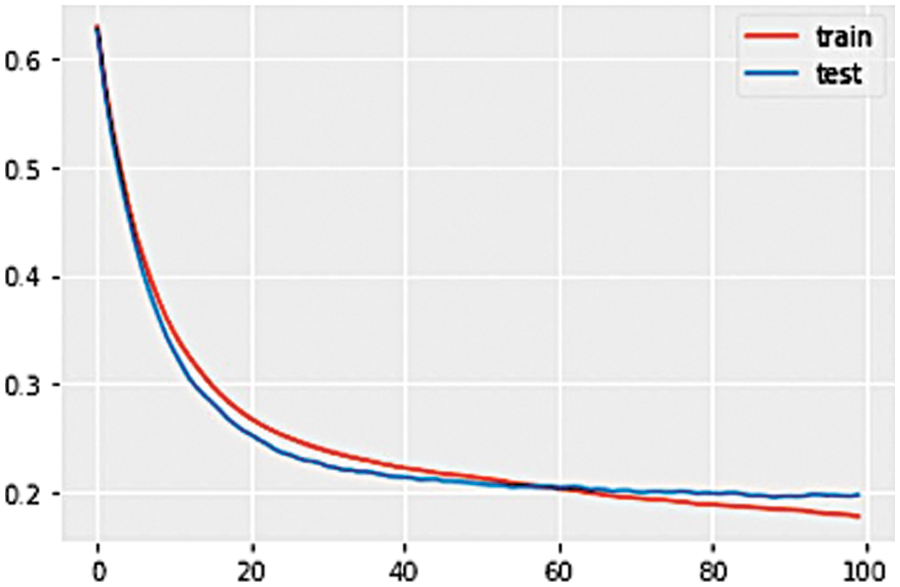
Figure 6: Learning curve for XGBoost model

The Authors have used the XGBoost loss function (binary: logistic) for binary classification and (multi: softprob) loss function for multiclass classification.

6.2 ROC (Receiver Operating Characteristic) Curve

ROC graph displays a model’s performance across all categorization levels. We see two parameters in this true positive rate and false positive rate (see Figs. 7–11).

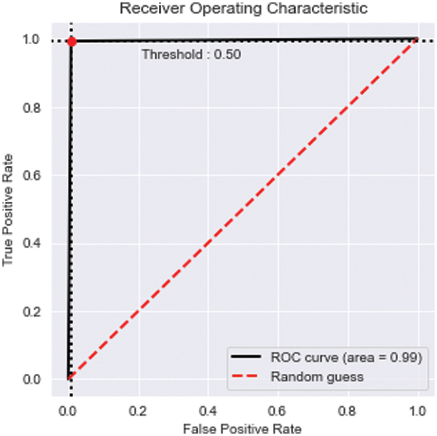
Figure 7: ROC curve for XGBoost

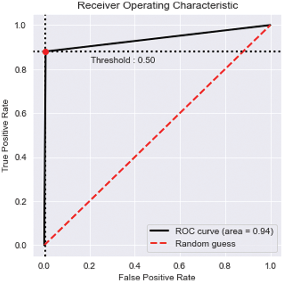
Figure 8: ROC curve for SVM

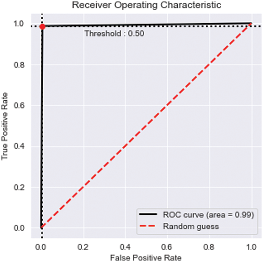
Figure 9: ROC curve for RF

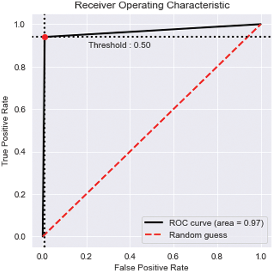
Figure 10: ROC curve for DT

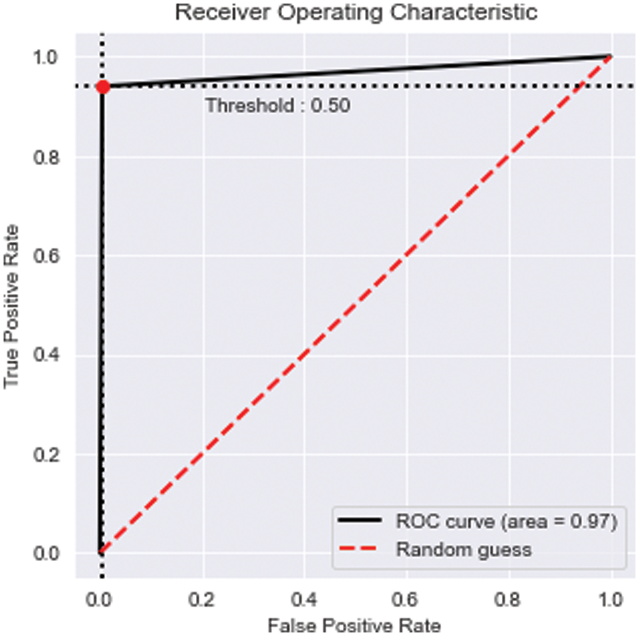
Figure 11: ROC curve for LR

7  Comparative Analysis

The Authors have incorporated many machine and deep learning methods for comparison purposes. Algorithms like a Decision tree and Random Forest tend to reduce the variance, leading to underfitting. At the same time, gradient boosting enhances bias by enabling to indict individuals who do not enhance the model. In contrast to XGBoost, which decides what direction to follow for missing values, SVM struggles with missing data. Logistic regression works fine on linear data, but generally, we don’t see linear data in the real world; no limitation in XGBoost like this. When XGBoost accomplishes the proper attribute adjustment, XGBoost outperformed the LSTM strategy in precision and speed. The present work with the XGBoost model achieved an accuracy of 99 % on the sensor weather data of the Lucknow Table 3.

8  Conclusions

The paper aims to generate accurate weather forecasts through inexpensive sensors. Satellite data cannot effectively cover a small building or a small region because the weather-affecting parameters change very frequently within a short distance. The Authors have collected data in real-time using a variety of sensors and applied different machine-learning algorithms to test and validate. The Authors also verified that the same algorithm produces different results for varying geographic locations. At, the last the Authors concluded that among Decision Tree, Random Forest Classifier, ANN, SVM, XGBoost, and logistic regression, the XGBoost based method produced the best results. In the future, the Authors will attempt to make predictions through transformer neural networks as in the transformer model, the Authors process data parallelly, leading to fast processing.

Funding Statement: The authors received no specific funding for this study.

Author Contributions: K. Y. conceptualized, designed, collected the data & performed the experiments, and contributed to the preparation of the draft manuscript. A. S. conceptualized, designed, collected the data, and contributed to the preparation of the draft manuscript. A. K. T conceptualized, designed, and supervised the study as well as reviewed and edited the final manuscript. All the Authors read and approved the final manuscript.

Conflicts of Interest: The authors declare that they have no conflicts of interest to report regarding the present study.

References

1. M. Chen, F. Herrera and K. Hwang, “Cognitive computing: Architecture, technologies and intelligent applications,” IEEE Access, vol. 6, pp. 19774–19783, 2018. [Google Scholar]

2. A. F. Pauzi and M. Z. Hasan, “Development of IoT based weather reporting system,” Proceeding IOP Conference Series: Materials Science and Engineering, vol. 917, no. 1, pp. 012032, 2020. [Google Scholar]

3. S. S. Bhatkande and R. G. Hubballi, “IJARCCE weather prediction based on decision tree algorithm using data mining techniques,” International Journal of Advanced Research in Computer and Communication Engineering, vol. 5, no. 5, pp. 483–487, 2016. [Google Scholar]

4. R. K. Yadav and R. Khatri, “A weather forecasting model using the data mining technique,” International Journal of Computer Applications, vol. 139, no. 14, pp. 4–12, 2016. [Google Scholar]

5. N. Jantakoon, “Statistics model for meteorological forecasting using fuzzy logic model,” Mathematics and Statistics, vol. 4, no. 4, pp. 95–100, 2016. [Google Scholar]

6. A. R. Gurung, “Forecasting weather system using artificial neural network (ANNA survey paper,” International Journal of Latest Engineering Research and Applications, vol. 2, no. 10, pp. 42–50, 2017. [Google Scholar]

7. M. Dragoni and M. Rospocher, “Applied cognitive computing: Challenges, approaches, and real-world experiences,” Progress in Artificial Intelligence, vol. 7, no. 4, pp. 249–250, 2018. [Google Scholar]

8. S. Madan, P. Kumar, S. Rawat and T. Choudhury, “Analysis of weather prediction using machine learning big data,” in Proc. Int. Conf. on Advances in Computing and Communication Engineering, Paris, France, pp. 259–264, 2018. [Google Scholar]

9. R. Bhardwaj and V. Duhoon, “Weather forecasting using soft computing techniques,” in Proc. Int. Conf. on Computing, Power and Communication Technologies, GUCON 2018, New Delhi, India, pp. 1111–1115, 2019. [Google Scholar]

10. M. Mohammadi, A. Al-Fuqaha, S. Sorour and M. Guizani, “Deep learning for IoT big data and streaming analytics: A survey,” IEEE Communications Surveys and Tutorials, vol. 20, no. 4, pp. 2923–2960, 2018. [Google Scholar]

11. G. Verma, P. Mittal and S. Farheen, “Real time weather prediction system using IoT and machine learning,” in Proc. 6th Int. Conf. on Signal Processing and Communication, ICSC 2020, Noida, India, pp. 322–324, 2020. [Google Scholar]

12. K. Ioannou, D. Karampatzakis, P. Amanatidis, V. Aggelopoulos and I. Karmiris, “Low-cost automatic weather stations in the Internet of Things,” Information (Switzerland), vol. 12, no. 4, pp. 146, MDPI AG, 2021. [Google Scholar]

13. P. Hewage, M. Trovati, E. Pereira and A. Behera, “Deep learning-based effective fine-grained weather forecasting model,” Pattern Analysis and Applications, vol. 24, no. 1, pp. 343–366, 2021. [Google Scholar]

14. Z. Q. Huang, Y. C. Chen and C. Y. Wen, “Real-time weather monitoring and prediction using city buses and machine learning,” Sensors, vol. 20, no. 18, pp. 1–21, 2020. [Google Scholar]

15. M. O. Osifeko, G. P. Hancke and A. M. Abu-Mahfouz, “Artificial intelligence techniques for cognitive sensing in future IoT: State-of-the-Art, potentials, and challenges,” Journal of Sensor and Actuator Networks, vol. 9, no. 2, pp. 21, 2020. [Google Scholar]

16. A. I. A. Osman, A. N. Ahmed, M. F. Chow, Y. F. Huang and A. El-Shafie, “Extreme gradient boosting (Xgboost) model to predict the groundwater levels in Selangor Malaysia,” Ain Shams Engineering Journal, vol. 12, no. 2, pp. 1545–1556, 2021. [Google Scholar]

17. K. U. Jaseena and B. C. Kovoor, “Deterministic weather forecasting models based on intelligent predictors: A survey,” Journal of King Saud University—Computer and Information Sciences, King Saud bin Abdulaziz University, vol. 34, pp. 3393–3412, 2020. [Google Scholar]

18. S. Lee, Y. S. Lee and Y. Son, “Forecasting daily temperatures with different time interval data using deep neural networks,” Applied Sciences (Switzerland), vol. 10, no. 5, pp. 1609, 2020. [Google Scholar]

19. T. Arcomano, I. Szunyogh, J. Pathak, A. Wikner, B. R. Hunt et al., “A machine learning-based global atmospheric forecast model,” Geophysical Research Letters, vol. 47, no. 9, pp. 17, 2020. [Google Scholar]

20. A. Y. B. Animas, L. O. Oyedele, M. Bilal, T. D. Akinosho, J. M. D. Delgado et al., “Rainfall prediction: A comparative analysis of modern machine learning algorithms for time-series forecasting,” Machine Learning with Applications, vol. 7, no. 22, pp. 100204, 2022. [Google Scholar]

21. P. Sharma and S. Prakash, “Real time weather monitoring system using IoT,” in Proc. ITM Web of Conf., Mumbai, India, vol. 40, pp. 1006, 2021. [Google Scholar]

22. Q. A. Al-Haija, M. A. Smadi and S. Z. Sabatto, “Multi-class weather classification using ResNet-18 CNN for autonomous IoT and CPS applications,” in Proc. Int. Conf. on Computational Science and Computational Intelligence, Las Vegas, NV, USA, pp. 1586–1591, 2020. [Google Scholar]

23. Q. A. Al-Haija, “A stochastic estimation framework for yearly evolution of worldwide electricity consumption,” Forecasting, vol. 3, no. 2, pp. 256–266, 2021. [Google Scholar]

24. Q. A. Al-Haija, M. Gharaibeh and A. Odeh, “Detection in adverse weather conditions for autonomous vehicles via deep learning,” AI, vol. 3, no. 2, pp. 303–317, 2022. [Google Scholar]

25. B. Charbuty and A. Abdulazeez, “Classification based on decision tree algorithm for machine learning,” Journal of Applied Science and Technology Trends, vol. 2, no. 1, pp. 20–28, 2021. [Google Scholar]

26. “These data were obtained from the NASA Langley Research Center (LaRC) POWER Project funded through the NASA Earth Science/Applied Science Program,”. [Online]. Available: https://power.larc.nasa.gov/ [Google Scholar]

27. S. Celine, M. M. Dominic and M. S. Devi, “Logistic regression for employability prediction,” International Journal of Innovative Technology and Exploring Engineering, vol. 9, no. 3, pp. 2471–2478, 2020. [Google Scholar]

28. H. C. Kim, S. Pang, H. M. Je, D. Kim and S. Y. Bang, “Constructing support vector machine ensemble,” Pattern Recognition, vol. 36, no. 12, pp. 2757–2767, 2003. [Google Scholar]

29. S. B. Maind and P. Wankar, “Research_paper_on_basic_of_artificial_neural_network,” International Journal on Recent and Innovation Trends in Computing and Communication, vol. 2, no. 1, pp. 96–100, 2014. [Google Scholar]

30. M. Belgiu and L. Drăgu, “Random forest in remote sensing: A review of applications and future directions,” ISPRS Journal of Photogrammetry and Remote Sensing, vol. 114, no. Part A, pp. 24–31, 2016. [Google Scholar]

31. T. Chen and C. Guestrin, “XGBoost: A scalable tree boosting system,” in Proc. ACM SIGKDD Int. Conf. on Knowledge Discovery and Data Mining, San Francisco, California, USA, vol. 13–17, pp. 785–794, 2016. [Google Scholar]

32. M. Vakili, M. Ghamsari and M. Rezaei, “Performance analysis and comparison of machine and deep learning algorithms for IoT data classification,” arXiv preprint arXiv:2001.09636. [Google Scholar]

33. S. Poornima and M. Pushpalatha, “Prediction of rainfall using intensified LSTM based recurrent neural network with weighted linear units,” Atmosphere, vol. 10, no. 11, pp. 668, 2019. [Google Scholar]

34. B. M. Preethi, R. Gowtham, S. Aishvarya, S. Karthick and D. G. Sabareesh, “Rainfall prediction using machine learning and deep learning algorithms,” International Journal of Recent Technology and Engineering (IJRTE), vol. 10, no. 4, pp. 251–254, 2021. [Google Scholar]

35. N. Oswal, “Predicting rainfall using machine learning techniques,” arXiv preprint arXiv:1910.13827, 2019. [Online]. Available: https://doi.org/10.36227/techrxiv.14398304.v1 [Google Scholar] [CrossRef]