Classification of Multi-view Digital Mammogram Images Using SMO-WkNN

1  Introduction

BCa is one of the subtypes of cancer that has risen to the second leading cause of death among women. According to the world health organization (WHO), cancer is one of the diseases among the leading causes of death in 112 countries (of 183 total). There were reportedly 2,261,419 new cases of BCa diagnosed in the year 2020. This makes BCa the most frequent disease and accounts for 12.5 percent of all new patients diagnosed worldwide in the same year. BCa is the fifth leading cause of death worldwide, accountable for 685,000 deaths. According to the research conducted by “Statista” in 2020, the number of cases with a five-year prevalence rate in India was 4,59,271. BCa is expected to be the most common disease in India in 2020, with 1,78,361 newly diagnosed cases (13.5 percent) and 90,408 deaths as a direct result of the disease (10.5 percent), as shown in Fig. 1 [1].

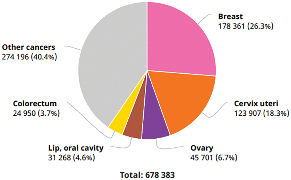
Figure 1: Number of new cancer cases in India in 2020

Patients diagnosed with BCa in India have a poor survival rate compared to those in western countries. This is due to many factors, including earlier age at disease onset, a later stage of disease diagnosis, a delay in the initiation of definitive management, and inadequate or fragmented treatment. Early detection and appropriate treatment are the most effective interventions for BCa control, as stated in the “World Cancer Report 2020” [1]. Having a history of BCa in one’s family, aging, changes in genes, race, being exposed to chest radiation, and obesity are all considered risk factors. The BCa patient’s survival rate could be increased with early detection screening methods. As a result, consistent screening is regarded as one of the essential techniques that could support the early identification of this kind of tumor. Mammography is the most effective screening modality for identifying BCa in its earlier phases. Mammograms could uncover a variety of breast abnormalities even before any symptoms manifest themselves. Most of the analyses proposed for BCa classification and detection made an effort to develop very effective CAD systems for BCa [2].

Breast tissues can be classified as normal, benign, or malignant based on abnormalities such as micro-calcifications, masses, architectural distortions, and asymmetries [3]. Normal breast tissue does not contain any abnormalities. The use of imaging equipment is recommended for both the detection and diagnosis of these anomalies. The imaging technique known as 2D mammography is utilized in most BCa screenings. Because it is an x-ray that is used to image the breast tissue, a mammogram is a screening method that does not involve invasive procedures. It can highlight the masses as well as the calcifications. In addition, it is considered to be a very sensitive and efficient screening approach. Mammography can support minimizing fatality rate through early identification of BCa even before any symptoms appear. Film mammography and digital mammography are the two available different kinds of mammography. Compared to film mammography, the digital mammogram’s sensitivity is much high in young women and people with dense breast tissue. It also requires a significant amount of storage space, along with having a low spatial resolution. Mammogram has an accuracy rate of 85 percent when detecting cancer in its earlier stages [4].

Ultrasound and magnetic resonance imaging (MRI) can be utilized as an alternative to mammograms, particularly with patients with highly dense tissues in the breast. However, this does not mean they could consider replacing mammograms [5]. Mammograms can be taken from several angles, each of which provides additional information that could support the identification and diagnosis of BCa. The CC and MLO views of mammography are the most important ones to analyze. As displayed in Fig. 2 [5], the breast is placed among the paddles for revealing the glandular tissues and fatty tissues in a CC view. The right segment of the CC views represents the chest muscle’s exterior edges. The CC views mammogram are captured horizontally from the upper projections at a C-arm angle of 0 degrees. The MLO view of mammography is acquired with the C-arm at a 45 degrees side angle; the breast was compressed diagonally among the paddles. As a result, imaging the breast tissue’s larger portion is possible as correlated with other views. Additionally, the MLO projection makes it possible for the pectoral muscle to be seen in the mammogram images [6].

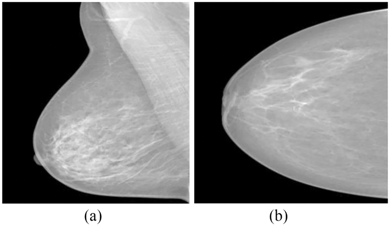
Figure 2: (a) MLO and (b) CC mammogram projections

Breast masses and calcifications are the two most common kinds of breast abnormalities detected by mammography. Breast masses can be cancerous or non-cancerous; cancerous tumors in mammography have uneven margins and spikes extending from the mass itself. Non-cancerous breast masses do not have these characteristics. Contrarily, the appearance of non-cancerous masses typically resembles that of a round or oval form with clearly defined edges. Calcifications in the breast can be divided into two different categories: micro and macro-calcifications. On mammography, macro-calcifications look like huge white dots scattered irregularly around the breast. These macro-calcifications are regarded to be non-cancerous cells. The micro-calcifications can be seen as tiny calcium spots that have the appearance of white specks. Additionally, they frequently appear in clusters. Micro-calcification is typically regarded as the main indication of early BCa or as the symptom of the presence of precancerous cells [7].

Recently, the field of artificial intelligence has witnessed a substantial increase in multi-view representation learning. In many existing studies, a BCa diagnosis was made based solely on the information from a single image of a mammogram. In multi-view CAD systems, radiologists typically employ the information from four different views of mammograms to conduct and improve the BCa prediction analysis. Mammograms for screening purposes often produce four x-ray images of both breasts or two views (MLO and CC) of each breast from various angles. The radiologist begins the analysis by analyzing the left central composite (LCC) perspective. If they see anything out of the ordinary in this view of the mammography, they will proceed to check the mammogram using the left MLO (LMLO), right CC (RCC), and right MLO (RMLO) views in that order. The presence of suspicious regions in these views represented in Fig. 3 [7] raises the probability of abnormalities. However, the performance of the CAD system can be improved by integrating the multi-view images of mammography at the same time [7]. This research proposes a DL-based CNN model to diagnose BCa from digitized mammogram images. This proposed model is a multi-view-based CAD model, which performs the diagnosis of BCa on multi-views of mammogram images like CC and MLO.

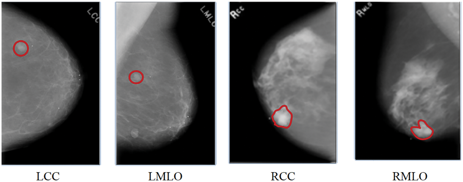
Figure 3: A mammogram of different views

2  Analysis of Related Works

The majority of CAD systems utilize mammographic views that are either CC or MLO. To make a proper diagnosis, it is important to examine both of these views (MLO and CC). The diagnosis of BCa was accomplished in [8] through statistical feature fusion methodologies. When fusing the textural features of these two views of mammographic images, the statistical feature fusion methods, including generalized discriminant analysis, principal component analysis (PCA), discriminant correlation analysis, and canonical correlation analysis, were utilized. Following the fusion of features, the support vector machine (SVM) was applied to classify the tumors as benign or malignant. Deep learning methods might have been used instead of an SVM to get better detection performance.

In order to make an accurate diagnosis of BCa, a CAD system was proposed in [9]. Image segmentation, feature extraction, and classification were tasks involved in this model. The two views from a mammogram were segmented using a method known as adaptive k-means clustering. During the feature extraction phase, the usual k-means clustering and the Gabor filter were utilized to extract the features of both the CC and MLO perspectives. In the end, a k-NN classifier was utilized for classification. The performance of this model could have been improved by increasing the images utilized for testing and training. The extreme learning machine (ELM) and the fused feature model of mammograms were utilized in [10] to create a BCa CAD model. This model combined the characteristics of single views with the contrasting characteristics of double views to create a fused feature. This fused feature model was optimized by using feature selection methods for the fused vectors, such as genetic algorithm selection, sequential forward selection, and impact value selection. As a result, the optimal feature vector was produced. The ELM classifier identified the anomalies associated with BCa with the optimal fused features. Compared with the sequential forward method and impact value, the genetic algorithm with ELM performed exceptionally well.

The implementation of a CNN model known as CoroNet was proposed in [11] for the automatic identification of BCa. The architecture of Xception was trained on the whole-image BCa based on mammography. In this analysis, high-resolution mammography images were employed; hence, the model used in this work needs to be upgraded to examine the features presented in these high-resolution mammograms properly. The classifications of BCa into normal, benign, and malignant forms utilizing mammography images were carried out in [12] by developing the CNN-based CAD system. This work used the images obtained from both views of mammography. This CNN model has eight fully connected (FC), four max-pooling, and four convolutional layers. The CLAHE method was utilized in the preprocessing step, and the region-expanding algorithm was utilized during the region of interest (ROI) segmentation. Following the segmentations, 14 textural characteristics and five geometric features were obtained. An optimal collection of features was chosen with the assistance of a genetic algorithm. A kNN classifier has been utilized for the classifications. It could have been possible to increase the performance of this model by utilizing a large set of images. In [13], a faster region-based CNN (FR-CNN) model was employed to develop a fully automated model for detecting masses in full-field digital mammograms. The transfer learning approach was used to fine-tune this FR-CNN model, which was pre-trained on the larger mammogram data set to identify masses in smaller data sets. The larger mammography data set was used to train the model. This model was limited to identify the masses in an image; however, it is possible to enhance it by classifying them as benign or malignant. A DL model was proposed in [14] as a method for diagnosing BCa using digital mammograms that were highly accurate and required a relatively short amount of processing effort. This model was developed for BCa image segmentation and classification utilizing various pre-trained architectures, such as DenseNet-121, Inception-v3, VGG-16, Mobile-Net-v2, and ResNet-50. The U-Net modified approach was utilized to partition the chest regions from the mammography image, and the pre-trained models were applied for the classification process.

In [15], a CNN model based on DL was developed to solve the problems of classifying mammography tests containing images with multi-views and segmentation maps of breast lesions (i.e., micro-calcifications and masses). This model was initially pre-trained with exceptionally large computer vision training sets. Subsequently, it was fine-tuned with CC and MLO mammography views to classify mammogram tests. This model, which was randomly initialized, has a greater chance of overfitting the training data. A CAD system proposed in [16] improved the diagnostic performance of BCa by combining the mammogram features from the CC and the MLO views. The k-means clustering and the Gabor filters were utilized during the preprocessing stage, and the genetic and PCA methods were utilized during the feature extraction stage. The breast masses were classified with the help of a multilayer perceptron (MLP) neural network that had a single hidden layer and used the backpropagation learning approach. Compared to the genetic algorithm, the combination of k-means clustering, Gabor filters, and PCA produced good results. Implementing an optimization algorithm could have been able to produce better results in terms of performance. A deep CNN model, pyramid-CNN, was proposed in [17] to differentiate between normal and abnormal tissues of the breast. The representation of the gaussian pyramid was used for the analysis of multi-scale, and the model used pyramid-CNN. This model was a multi-scale feature discrimination approach that can be applied practically to recognize mammographic patterns. It was produced using a combination of the hessian operator determinant to select representative candidates, representations of the gaussian pyramid for multi-scale analysis, and a CNN model for identifying five different types of BCa structures. In order to prevent overfitting, a data augmentation strategy was used primarily based on sub-histogram equalization and geometric transformation. In [18], a multi-view feature fusion-based CAD system for the classification of mammography images was proposed. This system used the feature fusion technique of four different perspectives. On each view, a CNN-based feature extraction model was operated on it. For the purpose of making a final classification, these retrieved features were combined into a single layer. It could have been possible to segment the data and use pre-trained weights while extracting features, which would have resulted in better performance.

3  Proposed Methodology: A Multi-View-based CAD Model

A multi-view-based CAD model is proposed in this research, which performs the diagnosis of BCa on multi-views of mammogram images like MLO and CC. As displayed in Fig. 4, median filtering and CLAHE techniques are utilized for image enhancement in preprocessing stage. The segmentation is performed using the RG algorithm. The feature extraction is carried out from the segmented images using the PHOG and AlextNet models. Finally, the classification is performed using the SMO-WkNN.

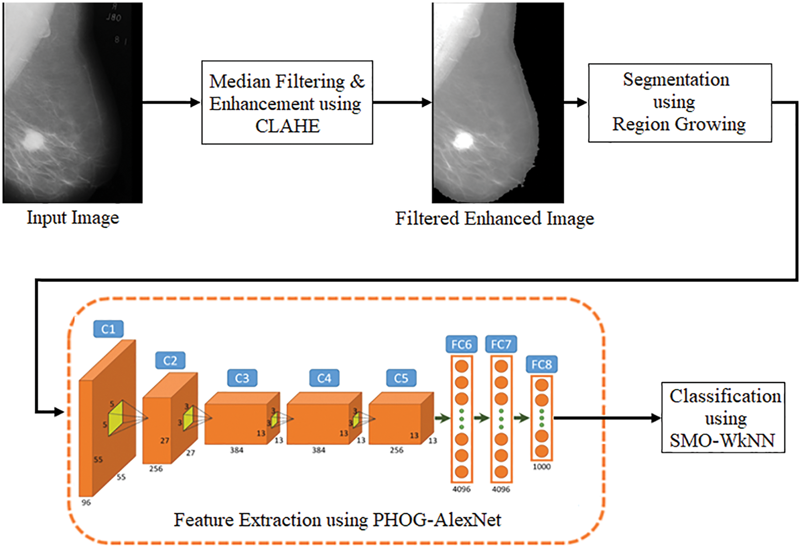
Figure 4: Pipeline of the proposed model

3.1 Image Preprocessing

Medical images sometimes have low contrast and are frequently affected by noise due to various sources of interference. These sources include the imaging process and data collecting. Consequently, it might become more challenging to assess them visually. Contrast enhancement techniques can significantly enhance image quality, providing medical professionals with a more easily interpretable image. In addition to this, it has the potential to improve the efficiency of deep recognition systems. Image enhancement is an effective image-processing approach that highlights critical information in an image and minimizes or removes certain secondary information to increase the identification quality in the process. This is accomplished through the process of highlighting certain secondary information. This work uses CLAHE, which uses a threshold parameter to restrict the level of enhancing contrast that could be generated inside the chosen region [19]. In addition, the image details’ clarity has been significantly improved. The CLAHE and median filtering techniques are utilized in the first stage of this model’s preprocessing procedure.

3.1.1 CLAHE

CLAHE is the improved variant of adaptive histogram equalization in which the contrast amplification is restricted to mitigate noise amplification. This is done to improve image quality [19]. In this particular analysis, CLAHE was utilized to improve the contrast as well as the characteristics of the image by making anomalies more readily apparent. The first step involves decomposing the mammography images into equally sized rectangular blocks and adjusting the histogram. The cumulative distribution function is used to carry out the mapping function in the histogram that has been clipped. The clip point can be computed by the mathematical equation expressed in Eq. (1).

α=SNi(1+β100Maxslope) (1)

where S is the total count of pixels, Ni denotes the dynamic range of pixels contained within each block, β denotes the clip factor, and Maxslope denotes the maximum slope, respectively. Eq. (2) represents the mapping function for the cumulative distribution function used to remap the blocks of the image in the grayscale image.

fCDF=∑z=0a⁡lpdf (2)

In this context, the term f refers to the pixel grey level, and fCDF stands for the cumulative distribution function.

The remapping function, together with the corresponding mathematical equation, is displayed in Eq. (3).

fremap=fCDF×maxl (3)

Here, the value denoted by maxl indicates the highest possible pixel count for each of the blocks. The mammogram was segmented into many contextual zones of identical size that did not overlap with one another. The histogram for each contextual zone was subsequently computed after that. In order to clip histograms, a clip limit with the value t = 0.001 was set. The clip limit was a threshold setting that allowed for the effective modification of the image’s contrast; increasing the clip limit resulted in an increase in the mammogram’s contrast. Each histogram’s data was reorganized to ensure that the clip limit was not exceeded in height. The transformation function was applied to each histogram; the results are shown in Eq. (4).

t(rk)=∑j=0k⁡pr(rj) (4)

Here, pr(rj)=njn was the probability density function of the grayscale value j in the mammography image input, n was the pixel’s total number in the mammogram image input, and nj was the pixel’s count in the input corresponded to the grayscale value j . The neighbouring tiles were joined using a bilinear interpolation technique, and the mammography images’ grayscale values were adjusted according to the histogram modifications [20].

3.1.2 Median Filtering

The implementation of filtering techniques has improved image quality, elimination of noise, and preservation of an image’s edges. A nonlinear filter method called the median filter was utilized to enhance the image quality and eliminate salt and pepper noises. This filter method works to preserve edges, which are the most significant aspect of a visual appearance. This filter replaces all pixel values with the median of neighbouring pixel values. The median filter is a low-pass filter that eliminates noise while still maintaining the image’s original details. The median filter filters a neighbourhood m × n by first positioning all of the neighbourhoods in descending order, then selecting the element in the middle of the ordered numbers, and then replacing the pixel in the image’s center [21]. The median filter is described by the mathematical equation, which is represented in Eq. (5).

x(m,n)=median(y(i, j),(i,j)∈N) (5)

In this context, N refers to the neighbourhood in an image centered on the coordinates (m, n). The salt and pepper noises can be effectively eliminated by utilizing the median filter. The noise present in the mammography is cleaned up with the help of the median filter in this work. [m, n] = [3] is the size picked for the median filter mask.

3.2 Segmentation Using Region Growing

The process of image segmentation using the RG algorithm is a basic region-based technique. Because it requires the selection of initial seed points, it is also categorized as a pixel-based image segmentation approach. This segmentation method evaluates the pixels near the initial seed points to determine whether or not those pixels’ neighbours should be added to the region. The selection of a seed point, which serves as the beginning point from which a region will grow, is critically significant to the final segmentation result. If a seed point is chosen from beyond the ROI, the conclusion of the segmentation process will unquestionably produce an inaccurate result [22].

This technique takes advantage of the crucial feature that pixels that are physically close to one another tend to have comparable grey values. The technique begins with a single pixel, referred to as the seed, and hence it extends the region surrounding the seeds to involve neighbouring pixels present in the threshold range. The following is a brief of the primary steps.

Step 1: Select the seed pixels. The seed was selected manually, about in the middle of mass, and its value was adjusted to be equal to the 15 × 15 pixel’s average. The seed pixel’s local intensity will not affect the growing process.

Step 2: Check the neighboring pixel values and include them in the region if they have a high degree of similarity to a seed. The similarity condition uses thresholds referred to as Th1 and Th2.

Th1=I−(0.3−K)⋅I¯ ; Th2=I+(0.3−K)⋅I¯ (6)

where I¯ was the average brightness value in the segmented zones, which shifts at every new growth stage, and K was the parameter dependent on both the brightness and the distance from the seed. It is possible to arrive at an appropriate value for K by the regression analysis of the values of K that correspond to the best shape selected by the radiologists:

K=0.097+1.330⋅F (7)

This value is contingent on the presence of factor F, which can be described as follows:

F=dN⋅(Imax−Iseed) (8)

where d was the distance between the initial seed and the ROI pixel that has the maximum brightness, Iseed was the luminance of the initial seed, Imax was the maximum brightness of the ROI, and N × N was the ROI size. It is necessary to repeat step 2 for every recently included pixel. End if no additional pixels cannot be included [23]. As per the segmentation process, Fig. 5 represents the segmented images of different views.

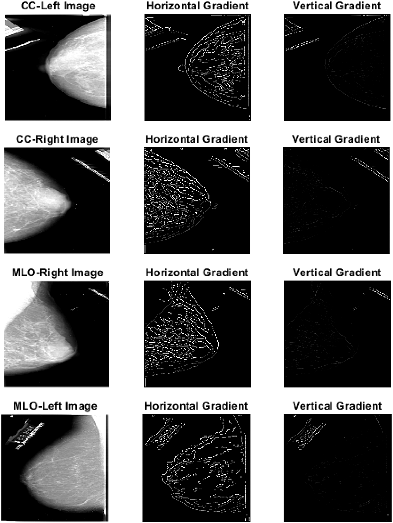
Figure 5: Segmented images using region growing

3.3 Feature Extraction Using PHOG-AlexNet

In this proposed model, an additional processing called feature extraction is performed after the malignant area has been segmented using image segmentation to acquire accurate results. In order to represent the local shape descriptor, the PHOG features are utilized. An image is to be represented by its local shapes and the spatial layout of the shapes. Then, the local shape of an area is determined by the distribution of edge orientations inside that area. At the same time, the spatial layout is determined by tiling the images into sections of varying resolution. A histogram of orientation gradients is included in the PHOG descriptor. This histogram is calculated for every picture’s sub-region and resolution level. In order to accomplish this, each image is split into a series of progressively more precise spatial grids. This is accomplished by repeatedly increasing the count of divisions along each axis. The pyramid’s grid has 2l cells running along each dimension at level l. The PHOG descriptor of the complete image is a vector with the dimensions K∗∑l∈L⁡4l , where K represents the number of bins in the image. It is possible to produce a more local and discriminative representation of objects with a global measure. The PHOG descriptor is generated by merging the histograms of the edge orientations of all the cells [24].

AlexNet is a CNN-based architecture that has been pre-trained with the ImageNet database, which is used in this research. This model uses AlexNet and its five convolutions (Conv), five rectified linear units (ReLU), five max pooling, and two FC or dense layers. After being reduced in size to 224 × 224 pixels, images are to be given as input to AlexNet. The input image with dimensions 224 × 224 and three kernels, each measuring 11 × 11 × 3 pixels and a stride of four, is processed by the first Conv layer. The layer of the output is a 55 × 55 × 96 matrix. Max pooling and ReLU activation functions were utilized to integrate nonlinearity for the recovered features and reduce overfitting. The outcome has the dimensions 27 × 27 × 96. The output of the second Conv layer, which has 128 kernels with a 5 × 5 size and a stride of 1 × 1, is 27 × 27 × 128.

Similarly, Conv layers 3, 4, and 5 are applied with 384, 384, and 256 filters and a stride of 1 × 1. This is then trailed by the application of dropout, max pool, and padding. At last, the FC layers 6 and 7 yields 4096 features. Layer 1 provides the blob and edge of the input images, layer 2 executes the response to corners or conjunction of the edges and various edge or color conjunctions, layer 3 produces the texture of an image as its output, layer 5 identifies the various components of an object, and FC6, FC7, and FC8 are responsible for producing the image’s features [25]. Fig. 6 represents the histogram of features extracted using the model. The filters in the convolution layer with specific widths and heights on the input image are moved from the left to the right utilizing strides. The model’s complexity is simplified using convolution, which enables features to be learned from the models’ images. The following equation describes the convolution process. The convolution is determined as in Eq. (9) when the “R” image is given at the (i, j) dimension.

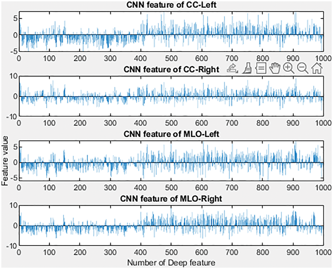
Figure 6: Features extracted based on CC and MLO views

F(i,j)=(R∗w)(i,j)=∑x⁡∑y⁡R(i−x,j−y)w(x,y) (9)

The feature map is referred to as “F” in the equation, while the convolution core along the x and y axes is referred to as “w.” The first layer receives the input image, consisting of three color channels with a height and width of 227 pixels, respectively. The input image also has a height of 227 pixels. This image will be processed through a three-channel filter with a width of 11 pixels and a height of 11 pixels for each channel. In the first layer, 96 filters are used to process the image. The activation function is the next phase in the process. For activation purposes, the ReLUs are utilized. After the end of the convolution, any negative values present in the input data will be reset to zero. The deep network will be developed into a structure that is not linear. Eq. (10) describes the ReLU function.

ReLU(x)=max(x,0) (10)

Filters are applied in the following manner, just as they were in the first layer: 256 filters of 5 × 5 in the second layer, 384 filters of 3 × 3 in the third layer, 384 filters of 3 × 3 in the fourth layer, and 256 filters of 3 × 3 in the fifth layer. Moreover, the pooling operation is performed after each iteration of the convolution and ReLU processes. The elimination of unnecessary features is the primary objective of the pooling process. It does this by decreasing the width and height of the input image that will be passed to the next convolution layer. Additionally, it generates a value that indicates neighbouring pixel groups in the features map. The features map is 4 × 4, and the maximum pooling feature generates the possible value in each 2 × 2 block while minimizing the features’ overall sizes to a significant degree. The final three layers are FC layers. In the sixth and seventh layers, which are both fully connected, there is a total of 4096 neurons, and each is coupled to all the other neurons in the layer. The FC layer is the next step, coming after convolution, ReLU, and pooling procedures. Every neuron in this layer has a complete connection to all of the neurons in the layer below it [26]. There are 4096 neurons in AlexNet’s FC6 and FC7 layers, and all of these are fully connected to one another.

3.4 Classification Using SMO-WkNN

SVM is the algorithm that forms the basis of SMO, which is an optimization of SVM. SMO is an algorithm that breaks down the quadratic programming (QP) issue into its component and then solves those parts. The drawbacks of SVM are remedied by SMO, which solves QP problems within the SVM algorithm without using additional matrix space and repeatedly using the same numeric value for each subproblem. The WkNN will be trained as part of the SMO’s overall process. The SVM concept can be explained as follows: if there is a collection of data points denoted by {(Hε, wε)}εp , where Hε and ‘p’ refers to the input vector and all of the training data, and then the SVM concept has been fulfilled. Finding a solution to the following problem is similar to the technique involved in training SVM for classification [27].

Maximize: Q(δε)=∑ε=1p⁡δε−12∑ε=1p⁡∑μ=1p⁡δεδμwεwμk(Hε, Hμ) (11)

where k(Hε,Hμ ) , δε and ‘c’ respectively represent the kernel function, the lagrange multiplier, and the user-determined regularization constant. The Gaussian function is by far the most common type of kernel function. If the issue described in (11) is successfully fixed, the decision function described in (12) will determine a distinct data sequence to use as the class label.

function(H)=∑ε=1p⁡δεwεk(Hε,H )+b (12)

In optimizing a working set, a subset of the training data sequence is performed at each phase. All features are given the same importance in the WkNN algorithm, which improves the standard k-NN technique. Features in the feature space are given weights in the WkNN algorithm according to their position in the space. The “squared inverse” method is utilized to compute the distance weights applied to neighbours. This is a supervised learning algorithm, which means that in addition to the training dataset, the previously classified data is also utilized to classify the following data. By storing training samples as their projections on each feature dimension individually, this WkNN algorithm achieved faster classification. Because all of the projected values may be kept in a data structure that enables fast search, this makes it possible for the kNN method to classify a new sample a great deal more quickly than it would have been possible otherwise. In the beginning, the algorithm generates a series of predictions for each feature and then applies the kNN algorithm to the projections made on each feature. Because of this, the highest classification of an example is decided by each feature’s independent classifications through majority voting [28–35].

4  Experiment Analysis

The experiment was conducted on the PC with a 64-bit CPU, i7 processor operating on windows 11, with 16 GB RAM, utilizing the MATLAB & Simulink tool R2018a. The dataset was collected from the DDSM database and utilized in this research for evaluation purposes. For performance analysis, the datasets were split into 75% for training and 25% for testing. This dataset is publically available from the following website link http://marathon.csee.usf.edu/Mammography/Database.html.

4.1 DDSM Dataset

For diagnosing BCa and classifying the disease, the DDSM dataset is one the most utilized datasets for BCa-related analysis. It is the most comprehensive public database available, containing normal images, images with benign lesions, images with malignant lesions, and two image views from each breast (MLO and CC). The database contains 2,620 cases, each of which contains two image views, for a total of 10,480 images. The DDSM is a database for mammograms that are structured according to cases. A mammogram collection of the same patient from various perspectives and directions is referred to as a case. Each case is classified as either malignant, benign, or normal, and it comprises information about the patients and the mammography descriptions, including the breast density rate, the precise location, and the abnormality type. Additionally, the ground truth annotations that correlate to the benign and malignant instances are related to the cases.

4.2 Performance Metrics

Various performance metrics like accuracy, recall, precision, specificity, FPR, and f1-score as well as MCC are utilized to test the performance of the model. Based on the values of true positive (TP), true negative (TN), false positive (FP), and false negative (FN), the performance computations were computed. The following equations are used for the computations.

Accuracy=TP+TNTP+TN+FP+FN (13)

Recall=TPTP+FN (14)

Precision=TPTP+FP (15)

Specificity=TNTN+FP (16)

F1score=2×Precision×RecallPrecision+Recall (17)

MCC=(TP×TN)−(FP×FN)(TP+FP)(TP+FN)(TN+FP)(TN+FN) (18)

4.3 Discussion

Table 1 represents the performance analysis comparison of the proposed model with existing models. The performance of the proposed model for diagnosing BCa from the DDSM dataset images was experimented with in this section.

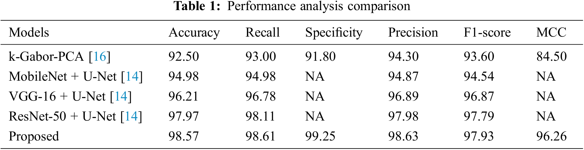
The proposed model’s performance was computed based on the parameters like accuracy, recall, specificity, MCC, f1-score, and precision. These computed measures were compared with the existing models like k-Gabor-PCA, MobileNet + U-Net, VGG-16 + U-Net, and ResNet-50 + U-Net for validation.

Accuracy is a metric that evaluates how many correct predictions a model was able to generate throughout the entirety of the test dataset. The research model obtained 98.57% accuracy, which is 0.6% to 6.07% higher than the compared models. Following the research model, the ResNet-50 + U-Net, VGG-16 + U-Net, and MobileNet + U-Net models obtained 97.97%, 96.21%, and 94.98% accuracy and the least accuracy was obtained by k-Gabor-PCA model with 92.50%. Fig. 7 represents the accuracy comparison.

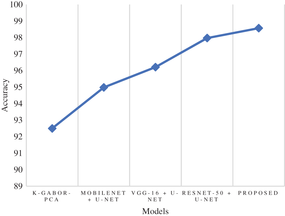
Figure 7: Comparison of accuracy

The true positive rate or recall is a measurement that determines how many true positives are predicted out of all the positives in the dataset. The recall rate of the research model was 98.61%, which is 0.5% to 5.6% improved than the other models in this research. The ResNet-50 + U-Net model has a close recall score compared with the research model, with 98.11%, and the k-Gabor-PCA model obtained the least recall score, with 94.98%. Fig. 8 represents the recall comparison. Specificity is measured as the proportion of actual negative results that match the expectations for those results (or true negative). This suggests that there will be some percentage of results that turn out to be negative even though they were anticipated to be positive. These results are sometimes referred to as false positives. The specificity rate of the research model was 99.25%, which is 7.45% improved than the k-Gabor-PCA model. The specificity score of ResNet-50 + U-Net, VGG-16 + U-Net, and MobileNet + U-Net models were not available for comparison. Fig. 9 represents the specificity comparison.

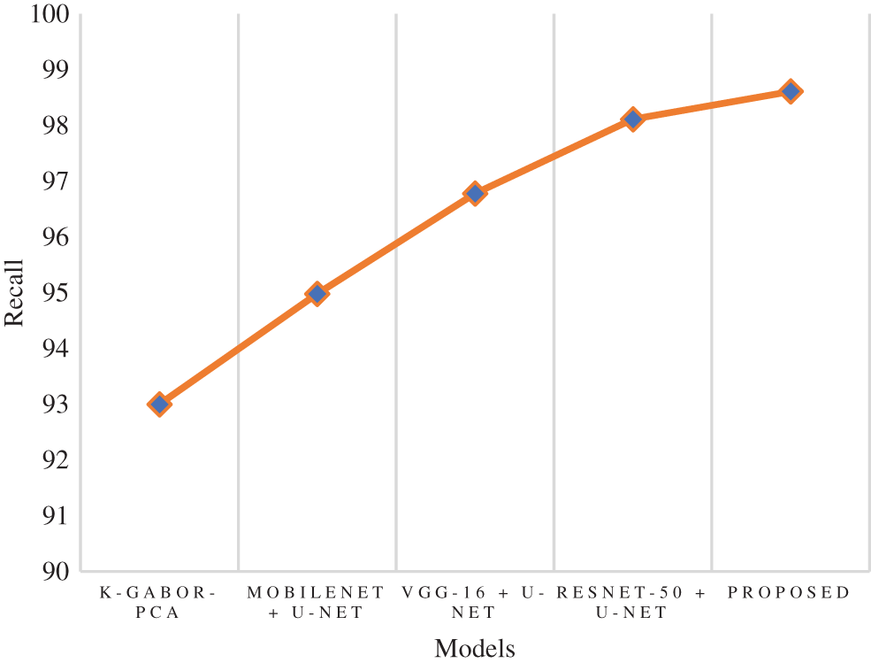
Figure 8: Comparison of recall

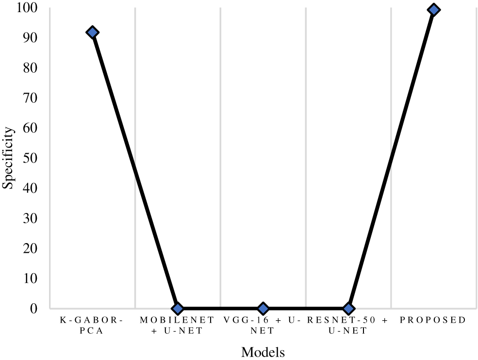
Figure 9: Comparison of specificity

Precision is a metric that can determine how accurate a positive prediction is. It is the proportion of TP relative to the aggregate of TP and FP. The research model obtained a 98.63% precision score, which is 0.65% to 4.33% improved than the compared models. Following the research model, the ResNet-50 + U-Net, VGG-16 + U-Net, and MobileNet + U-Net models obtained 97.98%, 96.89%, and 94.87% precision. The k-Gabor-PCA model obtained the least precision score of 94.30%. Fig. 10 represents the precision comparison.

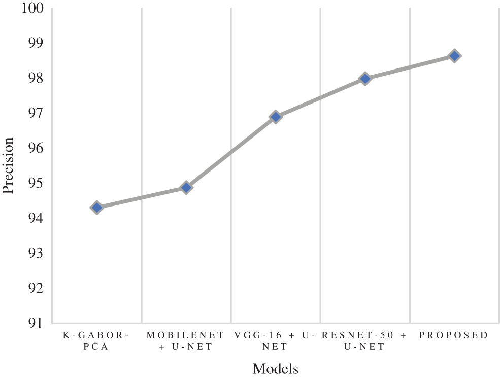
Figure 10: Comparison of precision

The f1-score is the harmonic mean of the recall and precision scores. It provides an estimate of the number of incorrectly classified instances that is more accurate than that provided by the accuracy metric. The research model obtained a 97.93% f1-score, which is 0.14% to 4.3% better than the compared models. Following the research model, the ResNet-50 + U-Net, VGG-16 + U-Net, and MobileNet + U-Net models obtained 97.79%, 96.87%, and 94.54% f1-score and the least f1-score score was obtained by k-Gabor-PCA model with 93.60%. Fig. 11 represents the f1-score comparison.

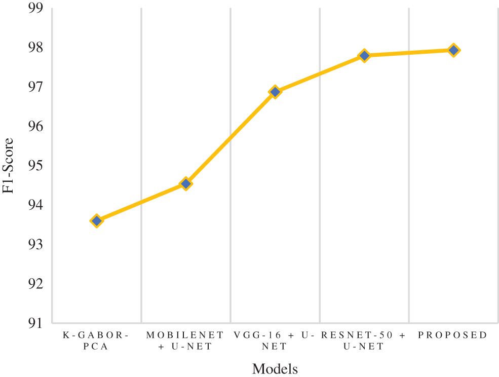
Figure 11: Comparison of f1-score

MCC is a model evaluation measure with a certain statistical value that generates a higher score only if a model obtained good results in each category (TP, TN, FP, and FN), proportional to the negative and positive factors in the data set. The MCC score of the research model was 96.26%, which is 11.7% higher than the k-Gabor-PCA model. The MCC score of ResNet-50 + U-Net, VGG-16 + U-Net, and MobileNet + U-Net models were not available for comparison. Fig. 12 represents the MCC comparison. The error rate and FPR of the proposed model’s performance were also calculated. The percentage of errors in a dataset is determined by taking the total number of wrong predictions and dividing it by the total number of data points. The best error rate was 0.0, whereas the worst possible was 1.0. The proposed model has an error rate of 0.0143. FPR is determined by dividing the total count of negative results by the count of incorrectly positive predictions made. The FPR can range anywhere from 0 to 1, with 0 being the best and 1 being the worst. The proposed model obtained an FPR of 0.0075. Based on the above comparison, it is clear that the proposed model has obtained greater performance results than the compared models in terms of all the output parameters.

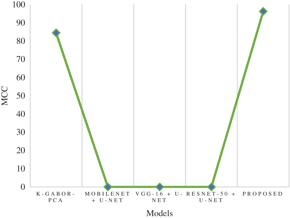
Figure 12: Comparison of MCC

5  Conclusion and Future Works

In this research, a multi-view-based CAD model was proposed to diagnose BCa. The multi-views of mammogram images include both left and right MLO and CC views of breast cancer digital images. The proposed model performed this research based on sequential stages like preprocessing, segmentation, feature extraction, and classification. The DDSM dataset was used for the evaluation of the proposed model. CLAHE and median filtering techniques were used for preprocessing and image enhancement. After preprocessing, the segmentation was performed using the RG algorithm. The feature extraction was carried out from the segmented images using PHOG and AlextNet models. Finally, the classification was performed using the SMO-WkNN optimized classifier. For training and testing, the dataset was divided into 75% and 25%. The classified images were evaluated based on accuracy, recall, precision, specificity, F1-score, and MCC. The proposed model’s error and false positive rates were also measured. The proposed model obtained 98.57% accuracy, 98.61% recall, 99.25% specificity, 98.63% precision, 97.93% f1-score, 96.26% MCC, 0.0143 error rate, and 0.0075 FPR. Compared to the existing models, the research model has obtained solid performances in all the evaluated parameters and outperformed the existing models. The limitations of this research include the usage of mammography and the proposed model’s higher specificity. However, mammography screening helps in early detection and reduces mortality, but it is an imperfect screening tool. In future, the proposed can be used for the imaging modalities used for breast cancer detection, such as MRI and Ultrasound. Additionally, state-of-the-art DL architectures can be implemented to classify and detect BCa as malignant or benign.

Funding Statement: The authors received no specific funding for this study.

Conflicts of Interest: The authors declare they have no conflicts of interest to report regarding the present study.

References

1. H. Sung, J. Ferlay, R. L. Siegel, M. Laversanne, I. Soerjomataram et al., “Global cancer statistics 2020: GLOBOCAN estimates of incidence and mortality worldwide for 36 cancers in 185 countries,” CA: A Cancer Journal for Clinicians, vol. 71, no. 3, pp. 209–249, 2021. [Google Scholar]
2. R. Mehrotra and K. Yadav, “Breast cancer in India: Present scenario and the challenges ahead,” World Journal of Clinical Oncology, vol. 13, no. 3, pp. 209–218, 2022. [Google Scholar]
3. A. Baccouche, B. G. Zapirain, Y. Zhen and A. S. Elmaghraby, “Early detection and classification of abnormality in prior mammograms using image-to-image translation and YOLO techniques,” Computer Methods and Programs in Biomedicine, vol. 221, no. 106884, pp. 1–17, 2022. [Google Scholar]
4. N. M. Hassan, S. Hamad and K. Mahar, “Mammogram breast cancer CAD systems for mass detection and classification: A review,” Multimedia Tools and Applications, vol. 81, no. 14, pp. 20043–20075, 2022. [Google Scholar]
5. A. B. Hollingsworth, “Redefining the sensitivity of screening mammography: A review,” The American Journal of Surgery, vol. 218, no. 2, pp. 411–418, 2019. [Google Scholar]
6. H. Bermenta, V. Becette, M. Mohallem, F. Ferreira and P. Chérel, “Masses in mammography: What are the underlying anatomopathological lesions?,” Diagnostic and Interventional Imaging, vol. 95, no. 2, pp. 124–133, 2014. [Google Scholar]
7. T. Tot, M. Gere, S. Hofmeyer, A. Bauer and U. Pellas, “The clinical value of detecting micro calcifications on a mammogram,” Seminars in Cancer Biology, vol. 72, no. 4, pp. 165–174, 2021. [Google Scholar]
8. S. Shanmugam, A. K. Shanmugam, B. Mayilswamy and E. Muthusamy, “Analyses of statistical feature fusion techniques in breast cancer detection,” International Journal of Applied Science and Engineering, vol. 17, pp. 311–317, 2020. [Google Scholar]
9. V. Sridevi and J. A. Samath, “Advancement on breast cancer detection using medio-lateral-oblique (MLO) and cranio-caudal (CC) features,” in Institute of Scholars (InSc), Coimbatore, India, pp. 1099–1106, 2020. [Google Scholar]
10. Z. Wang, Q. Qu, G. Yu and Y. Kang, “Breast tumor detection in double views mammography based on extreme learning machine,” Neural Computing and Applications, vol. 27, no. 1, pp. 227–240, 2016. [Google Scholar]
11. N. Mobark, S. Hamad and S. Z. Rida, “CoroNet: Deep neural network-based end-to-end training for breast cancer diagnosis,” Applied Sciences, vol. 12, no. 14, pp. 1–12, 2022. [Google Scholar]
12. V. S. Gnanasekaran, S. Joypaul, P. M. Sundaram and D. D. Chairman, “Deep learning algorithm for breast masses classification in mammograms,” IET Image Processing, vol. 14, no. 12, pp. 2860–2868, 2020. [Google Scholar]
13. R. Agarwal, O. Díaz, M. H. Yap, X. Lladó and R. Martí, “Deep learning for mass detection in full field digital mammograms,” Computers in Biology and Medicine, vol. 121, no. 103774, pp. 1–10, 2020. [Google Scholar]
14. W. M. Salama and M. H. Aly, “Deep learning in mammography images segmentation and classification: Automated CNN approach,” Alexandria Engineering Journal, vol. 60, no. 5, pp. 4701–4709, 2021. [Google Scholar]
15. G. Carneiro, J. Nascimento and A. P. Bradley, “Chapter 14-deep learning models for classifying mammogram exams containing unregistered multi-view images and segmentation maps of lesions,” in Deep Learning for Medical Image Analysis, Elsevier, Amsterdam, Netherlands, pp. 321–339, 2017. [Google Scholar]
16. S. Sasikala and M. Ezhilarasi, “Fusion of k‐Gabor features from medio‐lateral‐oblique and craniocaudal view mammograms for improved breast cancer diagnosis,” Journal of Cancer Research and Therapeutics, vol. 14, no. 5, pp. 1036–1041, 2018. [Google Scholar]
17. I. Bakkouri and K. Afdel, “Multi-scale CNN based on region proposals for efficient breast abnormality recognition,” Multimedia Tools and Applications, vol. 78, no. 10, pp. 12939–12960, 2019. [Google Scholar]
18. H. N. Khan, A. R. Shahid, B. Raza, A. H. Dar and H. Alquhayz, “Multi-view feature fusion based four views model for mammogram classification using convolutional neural network,” IEEE Access, vol. 7, pp. 165724–165733, 2019. [Google Scholar]
19. A. M. Tahir, Y. Qiblawey, A. Khandakar, T. Rahman, U. Khurshid et al., “Deep learning for reliable classification of COVID‐19, MERS, and SARS from chest x‐ray images,” Cognitive Computation, vol. 1, no. 5, pp. 1–21, 2022. [Google Scholar]
20. I. K. Maitra, S. Nag and S. K. Bandyopadhyay, “Technique for preprocessing of digital mammogram,” Computer Methods and Programs in Biomedicine, vol. 107, no. 2, pp. 175–188, 2012. [Google Scholar]
21. Z. Sha, L. Hu and B. D. Rouyendegh, “Deep learning and optimization algorithms for automatic breast cancer detection,” International Journal of Imaging Systems and Technology, vol. 30, no. 2, pp. 495–506, 2020. [Google Scholar]
22. J. Shan, H. D. Cheng and Y. Wang, “A completely automatic segmentation method for breast ultrasound images using region growing,” in Proceedings of the 11th Joint Conference on Information Sciences (JCIS 2008), Dordrecht, Netherlands, pp. 1–6, 2008. [Google Scholar]
23. G. Rabottino, A. Mencattini, M. Salmeri, F. Caselli and R. Lojacono, “Performance evaluation of a region growing procedure for mammographic breast lesion identification,” Computer Standards & Interfaces, vol. 33, no. 2, pp. 128–135, 2011. [Google Scholar]
24. P. P. Sarangi, B. S. P. Mishra and S. Dehuri, “Pyramid histogram of oriented gradients based human ear identification,” International Journal of Control Theory and Applications, vol. 15, no. 10, pp. 125–133, 2017. [Google Scholar]
25. K. Kavitha, B. T. Rao and B. Sandhya, “Evaluation of distance measures for feature-based image registration using AlexNet,” International Journal of Advanced Computer Science and Applications, vol. 9, no. 10, pp. 284–290, 2018. [Google Scholar]
26. F. A. Jokhio and A. Jokhio, “Image classification using AlexNet with SVM classifier and transfer learning, image classification using AlexNet with SVM classifier and transfer learning,” Journal of Information Communication Technologies and Robotic Applications, vol. 10, no. 1, pp. 44–51, 2019. [Google Scholar]
27. A. S. Hussein, R. S. Khairy, S. M. M. Najeeb and H. T. S. ALRikabi, “Credit card fraud detection using fuzzy rough nearest neighbor and sequential minimal optimization with logistic regression,” International Journal of Interactive Mobile Technologies, vol. 15, no. 5, pp. 24–41, 2021. [Google Scholar]
28. A. Sharma, R. Jigyasu, L. Mathew and S. Chatterji, “Bearing fault diagnosis using weighted k-nearest neighbor,” in Second International Conference on Trends in Electronics and Informatics (ICOEI), Tirunelveli, India, pp. 1132–1137, 2018. [Google Scholar]
29. T. Rajendran, P. Valsalan, J. Amutharaj, M. Jennifer, S. Rinesh et al., “Hyperspectral image classification model using squeeze and excitation network with deep learning,” Computational Intelligence and Neuroscience, vol. 2022, no. 9430779, pp. 1–9, 2022. [Google Scholar]
30. M. B. Sudan, M. Sinthuja, S. P. Raja, J. Amutharaj, G. C. P. Latha et al., “Segmentation and classification of glaucoma using u-net with deep learning model,” International Journal of Healthcare Engineering, vol. 2022, no. 1601354, pp. 1–10, 2022. [Google Scholar]
31. C. Narmatha and P. M. Surendra, “A review on prostate cancer detection using deep learning techniques,” Journal of Computational Science and Intelligent Technologies, vol. 1, no. 2, pp. 26–33, 2020. [Google Scholar]
32. S. Manimurugan, “Classification of Alzheimer’s disease from MRI images using CNN based pre-trained VGG-19 model,” Journal of Computational Science and Intelligent Technologies, vol. 1, no. 2, pp. 34–41, 2020. [Google Scholar]
33. R. S. Alharbi, H. A. Alsaadi, S. Manimurugan, T. Anitha and M. Dejene, “Multiclass classification for detection of COVID-19 infection in chest X-Rays using CNN,” Computational Intelligence and Neuroscience, vol. 2022, no. 3289809, pp. 1–11, 2022. [Google Scholar]
34. M. Shanmuganathan, S. Almutairi, M. M. Aborokbah, S. Ganesan and V. Ramachandran, “Review of advanced computational approaches on multiple sclerosis segmentation and classification,” IET Signal Processing, vol. 14, no. 6, pp. 333–341, 2020. [Google Scholar]
35. S. Sridhar, J. Amutharaj, P. Valsalan, B. Arthi, S. Ramkumar et al., “A torn acl mapping in knee mri images using deep convolution neural network with inceptionv3,” International Journal of Healthcare Engineering, vol. 2022, no. 7872500, pp. 1–9, 2022. [Google Scholar]
Cite This Article
Copyright © 2023 The Author(s). Published by Tech Science Press.
This work is licensed under a Creative Commons Attribution 4.0 International License , which permits unrestricted use, distribution, and reproduction in any medium, provided the original work is properly cited.
Downloads
Citation Tools