ILSM: Incorporated Lightweight Security Model for Improving QOS in WSN

1  Introduction

As an expeditious development in wireless communication technology, wireless sensor networks are gaining more importance in this era. Wireless sensor networks consist of several tiny nodes [1]. These nodes sense the data and transfer it to the next node according to governing rules. These rules are called routing protocols. In sensor nodes, sensory units are responsible for sensing the data from different environments as input and giving the desired output after processing [2]. All communication is based on wireless signals converted from analog to digital and vice-versa through an analog-to-digital converter. These are widely used in various industries, including urban military communication, environmental monitoring, tracking, smart agriculture, the Internet of Things (IoT), and many others [3,4]. Due to secure communication and efficient routing, sensor nodes have limited resources to transfer the data from source to destination [5]. Nodes have random behavior and arbitrarily disperse their signals, so achieving quality service in all aspects takes a lot of work. Security is also a crucial factor in wireless sensor networks [6]. Multiple cryptography techniques are used to secure the path; this overhead can delay communication [7]. There are many environmental issues, like fog, thunderstorm which cause to fade of the signals. Multiple techniques have been proposed to maintain and enhance the quality of services (QOS) of wireless sensor networks (WSN). Energy harvest in WSN (EHWSN) and energy harvest aware protocols have been used for clustering as the best way to achieve efficient routing mechanisms and tried to maintain the quality of service over all the WSN [8]. Nodes are consumed their energy for transmitting and receiving packets, so resultants are less energy and lead to poor communication and poor network lifetime. So an improved energy-aware routing model was proposed recently for improving load balancing and enhanced the lifetime of the WSN [9].

The main aim of this study is to propose an incorporated technique to provide an efficient routing mechanism with minimal overhead and maintain QOS parameters. In this paper, an Incorporated lightweight security model (ILSM) is proposed in which random waypoint mobility (RWM) model for path selection is used and manages node movements pattern to get efficient routing and minimal overhead in communication and grey wolf optimization (GWO) technique used to the optimized quality of service parameters.

The rest of the paper is organized as follows: Section 2 describes the proposed methodology, which is based on a hybrid model (RWP + GWO), and detail of the proposed algorithm. Section 3, named results, includes the performance of the proposed model and a comparative analysis with previous results. In the last Section, 4, the conclusion and future work are provided.

1.1 Background

After the brief introduction of WSN, the background of wireless sensor networks cover many aspects related to sensor networks and their parameters in different domain. Here are some highlights of WSN; where it started over time, ARPA (Advanced Research Project Agency)-Net was introduced; this agency was operational with 200 hosts in research institutes known as the first internet (World Wide Web). In contrast, the markets demand a more robust and extensive network covering the vast area network in wired architecture. Beyond these technologies, wireless networks were introduced as distributed/wireless sensor networks [10]. As technological advancement gradually increased, many organizations adopted the WSN approach for more reliable, speedy, and secure communication. Wireless sensor networks are widely used, as follows:

1.1.1 IoT in WSN

The Internet of Things (IoT) is a network of globally recognizable physical entities, their Internet integration, and their virtual or digital representation. A wide range of technologies is used to develop the Internet of Things. It is one of the most significant technological shifts in history, aiming to make everything intelligent, provide more innovative services, and develop new goods. IoT is a network of interconnected machines that exchange data and perform tasks by interacting with one another and with other items. This innovative technology was created to increase people’s quality of life and eliminate their direct interaction with the environment [11,12]. The internet of Things may be seen in road-car connections, home-city connections, and robot-factory links. In WSN sensors, small batteries are used and encouraged to develop efficient communication mechanisms. Energy-efficient protocols help to justify the energy mechanisms [13,14].

1.1.2 Smart Agriculture by WSNs

Wireless sensor networks are also implemented in agriculture for various reasons. Suitable sensor collection assisted in the resolution of numerous agricultural issues. To regulate the irrigation process, assess the weather impact on the crops, and test the soil fertility using wireless sensor networks and devices. With WSN, agriculture now moved into a new age of farming and other related processes [15]. WSN is also providing optimal solutions in agriculture. A variety of sensors is used to deploy smart farming [16].

1.1.3 WSN in Military and Security Organizations

WSNs are also used in military and security systems to provide high safety and accurate operation levels for such essential organizations. The sensors may detect mines, find injured individuals, regulate various components, and ensure the proper operation of military equipment [17,18]. Organizations always try to secure their transmission by implementing air and applying multiple security protocols and cipher techniques [19,20].

2  Methodologies

The proposed methodology aims to provide an incorporated Quality of Serve (QoS) strategy in package delivery dependability, living nodes, energy cost, dead nodes, throughput, and power consumption in WSN is being provided; for this purpose, a random waypoint mobility model is used. The routing algorithm aims to strengthen the durability and trustworthiness based on WSNs where the sensors are placed from source to destination and protected data communication. Then used, the Optimal Path Routing Algorithm based on Grey Wolf Algorithm for security as an enhanced lightweight security model.

2.1 Initial Phase of Proposed Methodology

In previous papers, the Random Waypoint (RWP) Simulation as a Mobility Model begins informally in a simulated field. This research helps us determine the ideal path by applying Grey Wolf Optimization with RWP Model. In the random mobility point model, the mobility parameter’s uniform distribution differs significantly from a stationary distribution. Nodes are concentrated in the stationary distribution around the network center. Thus, the point selected by the node along the travel is longer. There are three different ways to initialize. After the simulation is performed, the first approach stores the position file. For each simulation, it must create a position file such as each simulation starts with the stationary distribution. The second technique indicates that the time for simulation starts at 1000 s to prevent the problem of creating. The situation in both cases is, how long do we have to throw them away.? The stationary distribution chooses the third approach position and node speed. Across this article, nodes are distributed in a two-dimensional area using the random mobility model. Due to its simplicity, this is the most popular form of mobility. Each node randomly selects a path, destination, and speed for its mobility pattern and pauses after its destination (called pause time), and selects a random path and destination again until the simulation stops. This pause is irrespective of direction and tempo (vary from [1, vmax]). There are three primary components in the RWP models: speed(s), direction(s), and break time (p). In the RWP model of the distribution of mobility nodes, mobility and direction parameters are executed alone.

2.1.1 Implementation of Random Waypoint Mobility Method

The mobility model selection is required to develop any network protocol or algorithm. The synthetic mobility model is suitable for the actual behavior of a network Random mobility point model is one of the models of synthetic mobility. To prevent the initialization problem, randomly select the speed and direction. Pause time is taken to ensure the stability of the network throughout the movement; see Fig. 1.

Figure 1: Implementation flowchart of RWM

2.1.2 Energy Model

The key source of electricity reduction in the network is data transmission and reception. Sensory nodes consume substantially less energy for detection and processing. In this work, we track the original radio-a model of energy reduction in the transfer of raw data as indicated below:

ETX=Lx(Eelec+ϵxxd2)(1)

ERX=Lx Eelec(2)

ETX=Lx(Eelec+ϵxxd4)(3)

ϵ1, ϵ2, ϵ3, and ϵ4 are employed as SN, RN, CH, and CCO node amplifiers. The short-distance energy reduction and remote communication are identified; see Eqs. (1)–(3)

2.1.3 Proposed Algorithm for RWM

1.   To simulate the proposed model, the random mobility model is used. Predefined ranges are utilized to move the nodes and speeds randomly. Procedure Node Selection and Routing Phase (Number of Nodes N, Cluster Heads CHs, Cluster Coordinators CCs, Numberof Clusters C)

2.   Network Deployment in the Static Area (Random Distribution of Nodes).

3.       Division of area into a number of Clusters C

4.          Declare Cluster ID (C0, C1, C2, … Cc)

5.          Distribute IDs to every cluster

6.          Declare Sensor Nodes (SN)

7.          Declare Local Cluster (C)

8.          Declare Cluster Head (CH)

9.          Declare Cluster Coordinator (CC)

10.  Declare T as Node traveling time in the network

11.  Declare Ø as the direction of a node in the network

12.  Declare V as velocity

13.  Step-1% Mbl (moving) Phase%

14.        X coordinaten = X coordinaten n-1 + Vn x T x cos Ø n

15.        Yn = Yn-1 + Vn x T x sin Ø n

16.  Step-2% Selection of (RN) %

17.     For each, cluster_id ≤ M do

18.         Random N Selection

19.  End for

20.  Step-3% Cluster Head & Coordinator Cluster Selection

21.     For each cluster, cluster_id ≤ M do

22.         elect CH and CC randomized in the local cluster, where Ch. Energy >= energy. Threshold

23.    The Number of CC in every cluster is >= cluster_id-1

24.         ch ɛ CH and cc ɛ CC

25.  End for

26.  Step-4% Route selection %

27.     For every cluster, cluster_id <= M do

28.         Transfer the packets from the local station to Base Station

29.         Send packets to the energy level

30.  End for

31.  Step-5 For each cluster, cluster_id ≤ M do

32.  If rn_en < en_Threshold then

33.      Go to R-N selection.

34.       If CH_energy and CC_energy < en_Threshold then

35.       Move to cluster H and CC selection.

36.    Else

37.       Go to Route Selection

38.        End if

39.  End for

40.  End Procedure

Performance Evaluation of the RWM Model

The mobility models outlined in this study are carried out in 03 parameters: source-to-destination (E-to-E) delay, throughput, and packet transfer ratios. All these parameters and mathematical equations are covered below, which are determined.

Throughput

Valid data provided to sinks from sensor nodes at a specific moment is called their (network) output. It will be quite crisp to start rounds in every protocol. Later the processing is minimized when the information is repeatedly reused. The performance S can be computed as:

S=∑k=0∞S(k).g(k)(4)

S is throughput, where S (k) is the total nodes, and g (k) is the total data sent from nodes.

E-to-E (Source-to-Destination) Delay

The period a node occupies for data transmission to the destination node is called an E-to-E delay time. A high source-to-destination delay value refers to the optimal cluster head selection. It can be calculated as:

Total delay=No. of hops(1st packet total delay)+ Transmission−(Transmission delay +Processing +Queuing)(5)

Packet Transfer Ratio

The Packet transfer ratio is defined as the number of packets transferred successfully to the destination; see Eq. (6), Ptransfer, for the total no. of packets transmitted by various nodes, Psent illustrated in the following equation:

Packet Delivery Ratio:Ptransfer∑i=1nPsent(6)

2.1.4 Simulation Scenarios

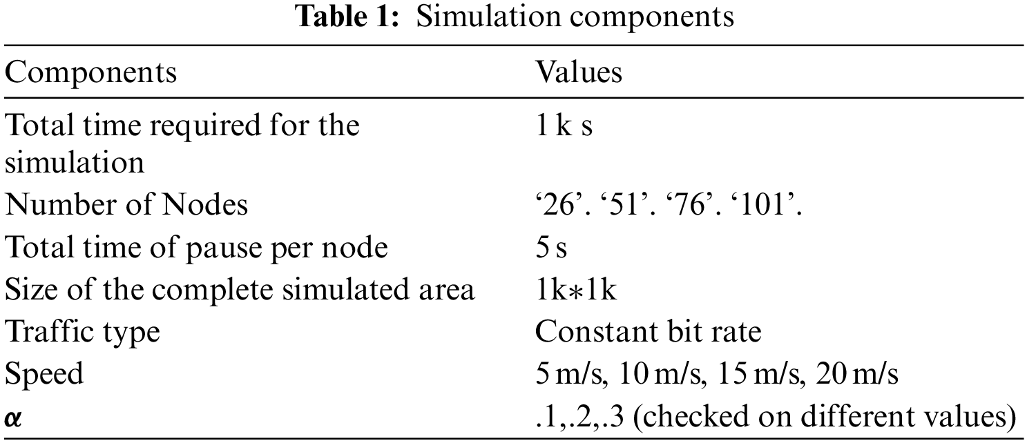
The mobility models discussed in this paper are built and evaluated using MATLAB simulation. Consequently, many scenarios have been provided to mimic the outcome of each mobility performance. Different network sizes are explored in various situations. To put it another way, network performance is assessed for each mobility model in this study utilizing a variety of network sizes. The 1st category contains static sensor nodes, whereas the 2nd comprises a mobile sink node that gathers data from the static sensor nodes. As a result, the total number of nodes in each scenario is n + 1 node. To be clear, the network size, in our case, is 26 nodes. As a result, 25 fixed sensor nodes and 1 mobile sink node exist. The mobile sink movement is investigated at three different speeds utilizing three other mobility models and varied network sizes. The simulation metrics are shown; see Table 1 below.

2.2 Second Phase of Proposed Model

2.2.1 Optimization Algorithms for Improvement of QoS for Optimal Path Selection

In the first step, each node in the network is chosen to be a cluster head (CH). Each node selects a value in each round (0–1). It is compared to Eq. (7). This node is taken as a CH for the present round if this value is less than the threshold [21].

T(n)={p1−p(r mod (1p)),ifnϵG0.otherwise(7)

Grey Wolf Optimization (GWO)

A new strategy named an incorporated lightweight model, “GWA’s RMW” model, is recommended to accomplish QoS for packet transferred reliability and electricity use in WSN. This routing approach focuses on enhancing life and dependability in WSNs. It relies on a direct connection between nodes, in which each node connects to the node next to it until it sinks. A one-hop or multi-hop from source to sink might occur depending on the distance between the source, the sink, and the transmission sensor. The sink node sends a query to each node to collect information about its (ID, position, and power condition). As a result, historical information on node distribution, field position, and power level status would be available. On their way from the source to the sinking node, nodes pass close together through nearby nodes. GWO algorithm is an intriguing algorithm because of the approach of group hunting. Based on Muro et al., grey wolf shooting is separated into three steps: to track, chase and approach the prey, (ii) pursue & encircle the prey until they stop; and (iii) attack the prey. In GWO, alpha, beta, and deltas are symbolically represented as and. Optimizing Grey Wolf contributes to both the investigation and utilization phases. It is used to seek the optimum result in a native hunt area. In grey wolves, the prey surrounding & beast attack are in phases of exploitation to investigate the ideal result in a small hunt area. This hunt acts as the phase of exploration during which the grey wolves search in a global search area for prey. The general mechanism of the Grey Wolf Algorithm is described in Fig. 2.

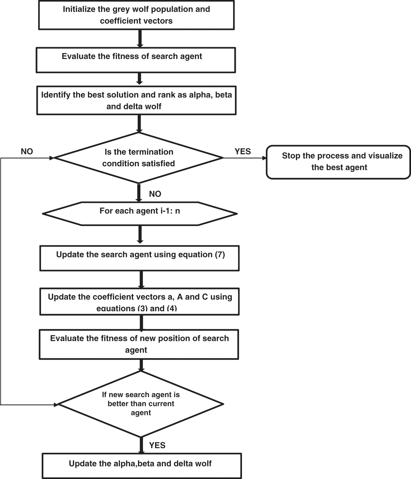
Figure 2: General mechanism of the Grey Wolf Algorithm (GWO)

2.2.2 Wireless Sensor Network Fitness Parameters

The fitness of a chromosome controls how much energy consumption is reduced and how much coverage is maximized [22]. Some essential fitness metrics are covered in the WSN below:

DDBS: it denotes the sum-of-neighbor distance between all sensor nodes and the BS represented by di as:

DDBS=∑1=1mdi(8)

where “m” is the limit of nodes

CD: total no. of CHs and BS distance and the sum of the distance b/w the resolute member nodes and their cluster heads:

CD=∑i=1n((∑j=1mdij)+Dis)(9)

2.2.3 Nodes Placement Using Grey Wolf Algorithm

The location of sensor nodes on a controlled field can impact the network’s overall performance. The placement of the deterrence node (grid), semi-deterministic nodes, and non-set nodes in the field are three major types of placement nodes in the network. A long-range sensor node’s transmission is inefficient because it requires more energy than a linear transmission distance function. Node density is only one aspect of network design, but it is essential in determining where a node should be placed.

The common advantages of proper sensor propagation are provided in WSNs below:

Scalability: When there are not infinite communications between nodes, a high number of nodes in the network may be installed

Reduction of Collision: Because the cluster head (CH) serves as the coordinator, only a few nodes have access to the channel and may communicate with other cluster members locally.

Efficiency in Energy: The periodically relocated results in high energy depletion. However, CH tasks may be dispersed among all other nodes by regular relocation, leading to lower energy depletion.

Low Cost: Additional expenditures are prevented by using sensors at the correct position.

Backbone Routing: the data are gathered in CH and transmitted to the sink by cluster members. Therefore, a minor traffic and routing backbone can be used to develop the network efficiently. Methodology for Grey Wolf Algorithm

A relay (active node) from the cluster architecture is designated the CH, and data is transferred to the spare nodes. Replacement nodes shall be utilized as replacement nodes if the following node or link fails. The following equation can find the radius of the district.

Rr=M×Mϕ×c(10)

where Rr is the neighborhood radius, M BM is the distribution area of SNs, and c is the number of clusters. The SN with more neighbors is picked as relay nodes during the selection procedure in the GWA. If the node fails, a previous node saves data in the buffer and chooses the next node to build a new path, as illustrated in the flowchart below. It depends on numerous criteria, such as the most significant residual energy for the next Hop SN, good connection quality, buffer size, and the lowest hops.

When selecting relay nodes from the GWA, each SN creates an arbitrary integer 0–1. The random number is matched the enhanced threshold when the random number is below the T (n); the SN is selected as an active node so that G is set to be stopping it from being reelection in this round as an active node [21]. We can describe G as a collection of SNs that marks the SNs that in the preceding 1/p rounds have not been selected as relay nodes:

T(n)={p1−p(r mod (1p))(dtsoBS avg− dtso BSidtsoBSavg)(Eint−EiEint)ifnϵG0.otherwise(11)

Suppose dtsoBSavg is the mean distance between SN and BS and dtsoBSiis the distance between SN number I and BS. In that case, Eint is the original energy, Ei is node energy, and p is the likelihood that n nodes should be chosen as a relay node. If the nodes are farther from BS, more energy is consumed to convey the data to BS.

2.3 ILSM Model Based on NS2

We performed these experiments on Network Simulator 2 (NS2). NS2 is used to validate the Lightweight Security model performance based on GWO. This simulator is object-oriented programming based. We have added the protocol detail to initiate system programming that will change the bytes and packet headers and implement the algorithm, which will run on the human body sensor values dataset. In this system, we will check the cluster head selection and calculate the energy consumption between nodes. Exponentially EWMA (Exponentially Weighted Moving Average) is used:

Eharvest (t,Psetup)=Z(t,Psetup)tλi(0) d0(12)

where Eharvest is the valued harvested energy by an sn I in a distinct time 0 period, and the charging rate of node I in time 0 is represented by λi(0).

Tool Command Language sets up different topologies, varying the number of nodes in a network.

In this paper, we developed a Model in NS2 by following these steps:

•   written the TCL code

•   Make the entry of each event (transmission of sensed data from the node) that occurred during simulation execution into a trace file.

•   Display a graphical form of the simulator model during execution using name trace.

•   Generate graphs based on trace file analysis and implement c++ codes for analysis & graph generation based on the dot.tr file.

In this research, we evaluated our model by calculating the following numbers of nodes:

Dead Nodes Numbers:

These nodes have energy, but they become dead by supplying energy. These tell us the total energy consumption in the VANETs.

Alive Nodes Numbers:

These nodes have energy, and they supply energy. After supplying energy, they have enough energy to survive. Alive node numbers are used to attain energy for the whole VANETS.

Cost Factor Calculation:

The optimum cluster head has been selected based on the information about energy loss, current energy, and other parameters. We calculate the total energy loss from GWO as follows:

Total Energy Loss = Loss of All Cluster Member + Loss of Sensor Node Energy

In these following energies and losses are calculated:

Energy Loss of cluster members:

Ec-mem(i)=∑j=1n{ Eamp x n x K x D(i,j) x E(tx) x K }(13)

Eamp x n x K x D(i,j)(D is the distance of node feom sink)x 

E(tx) are the total number of energies And Ec-mem (i) is the total energy loss of cluster members.

Energy loss for SN

ELoss-SN (i)=∑j=1N{(Etx−E(D−aggregation))Eampx n x K x D(i,sink) x E(rx)x K}(14)

where (Etx−E(D−aggregation))is the energy used in transmission and E(rx)is the energy used in reception

Sensor node energy

E(Total−curr(i))= ERes(i)+ EHarvest(i)(15)

Required Transmission power

TP=SNR∝(16)

where SNR is signal to noise ratio

3  Results

3.1 Random Waypoint Mobility

First, we have executed random waypoint mobility in the wireless sensor network; see Fig. 3 below.

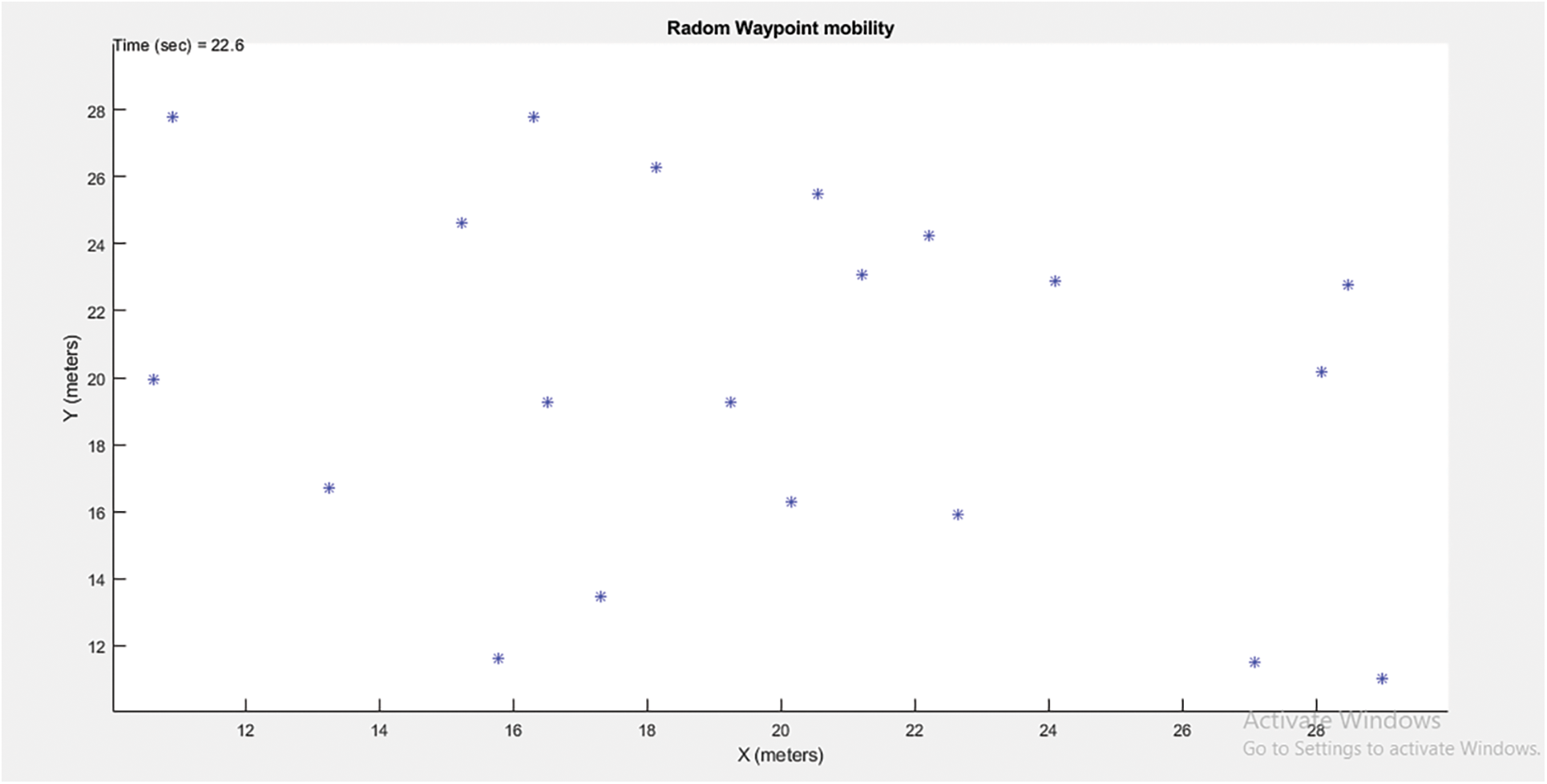
Figure 3: Random way point mobility

The mobility model selection is required to develop any network protocol or algorithm. The synthetic mobility model is suitable for a network’s actual behavior. The random mobility point model is one of the models of synthetic mobility. To prevent the initialization problem, randomly select the speed and direction. Pause time is taken to ensure the stability of the network throughout the movement.

Then after creating this, we calculated the performance of nodes as in E-to-E (source-to-destination delay, output, and packet transfer ratios and carried out some routing techniques which will help us in the Quality of Service.

3.2 Wireless Sensor Network Lifetime

The total working time of a network in terms of seconds is called network lifetime. It is considered the main evaluation parameter in wireless network systems in which nodes are involved as mobile sensors or battery-operated devices. The best network lifetime is responsible for the best wireless sensor network. Here in our case, we have compared the network lifetime of E-HARP with other state-of-the-art techniques, as shown in Fig. 4 below. E-HARP delivers the best performance concerning the number of rounds, and FPA shows the energy consumption of transmitting and receiving packets.

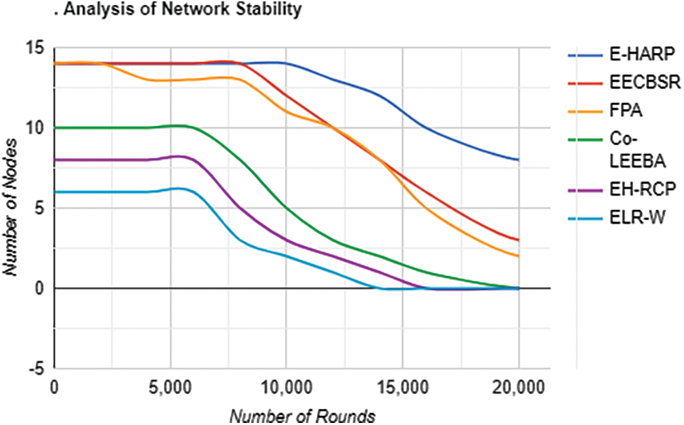
Figure 4: Analysis of network stability

Stability Period

Stability time is the time covering all the time of a network before the death of 1st sensor node. E-HARP’s 2nd protocol death occurs at the 7600th round, a value far greater than other techniques. This shows that our proposed protocol achieves the highest performance in stability. See Fig. 5.

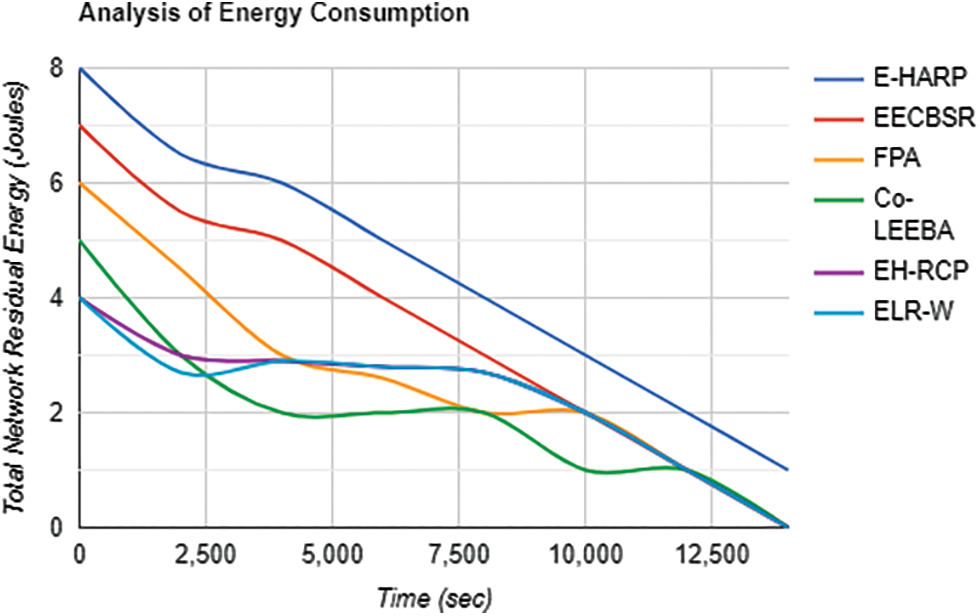
Figure 5: Stability period

Residual Energy

Residual energy is long-lasting energy at which the death of a sensor network occurs. The network energy of E-HARP shows that it attains maximum energy as compared to other techniques. Fig. 6 shows the graph of residual energy.

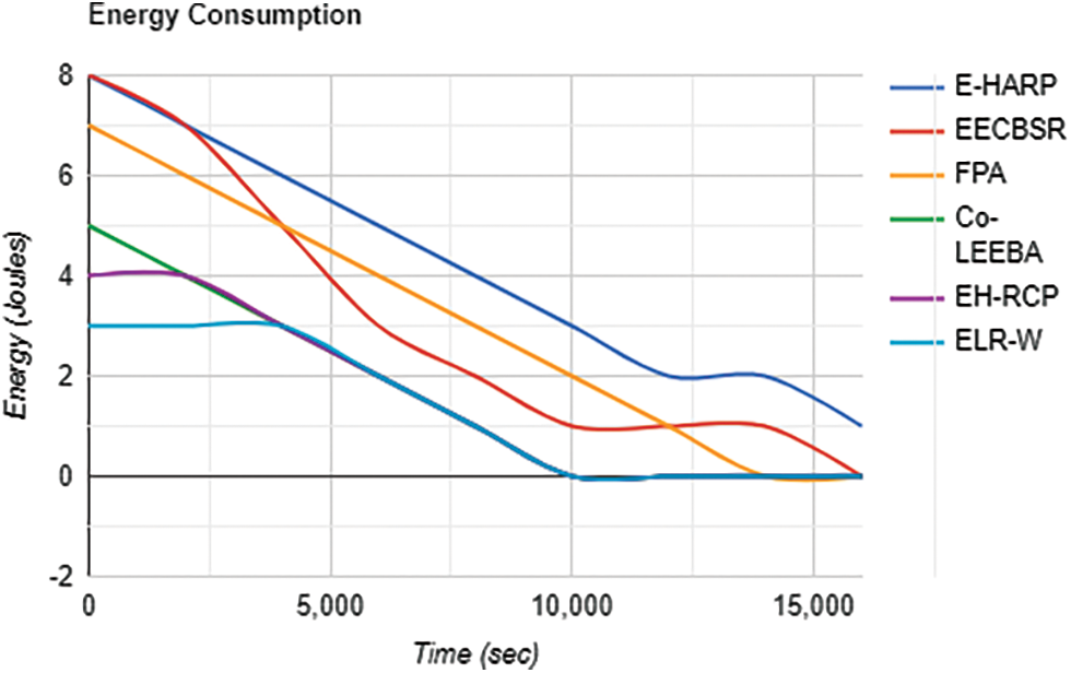
Figure 6: Residual energy

Throughput

Useful data sent to sink from sensor nodes in a specific time is called its (network’s) throughput. The throughput of E-Harp has shown the best among others. From 15000th onwards, starting rounds were too sharp. Later, the processing becomes minimized as the information is reused repeatedly (see Fig. 7).

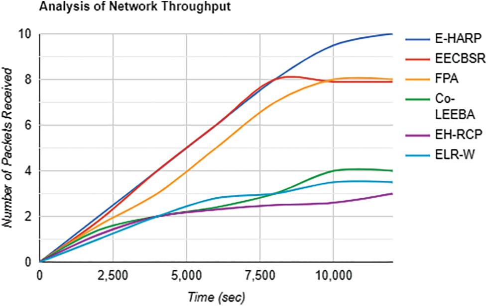
Figure 7: Throughput

E-to-E (End to End/Source to Destination Delay)

An E-to-E (source-to-destination delay time) is the time it takes a node to transmit data to a destination node. Compared to other methods, E-HARP offers the shortest E-to-E (source-to-destination) delay time while maintaining the highest power efficiency. The best cluster head selection is determined by a high value of the end-to-end delay, as shown in Fig. 8.

Figure 8: E-to-E (end-to-end delay/source-to-destination delay)

3.3 Grey Wolf Optimization

After implementing the RWP Model using Routing techniques, apply Grey Wolf Optimization to produce Lightweight Model for Quality of Service in a Wireless Sensor Network.

There is a 3-dimension surface plot of the tested grey wolf parameters (alpha, beta, and delta) functions in parameter spaces: f10(sum)=sum(x;y;z)=(7.5+4+15.7069),x1,x2€[−20,20] the area where the grey wolf optimization technique finds the best place to hunt the node, see Fig. 9 above.

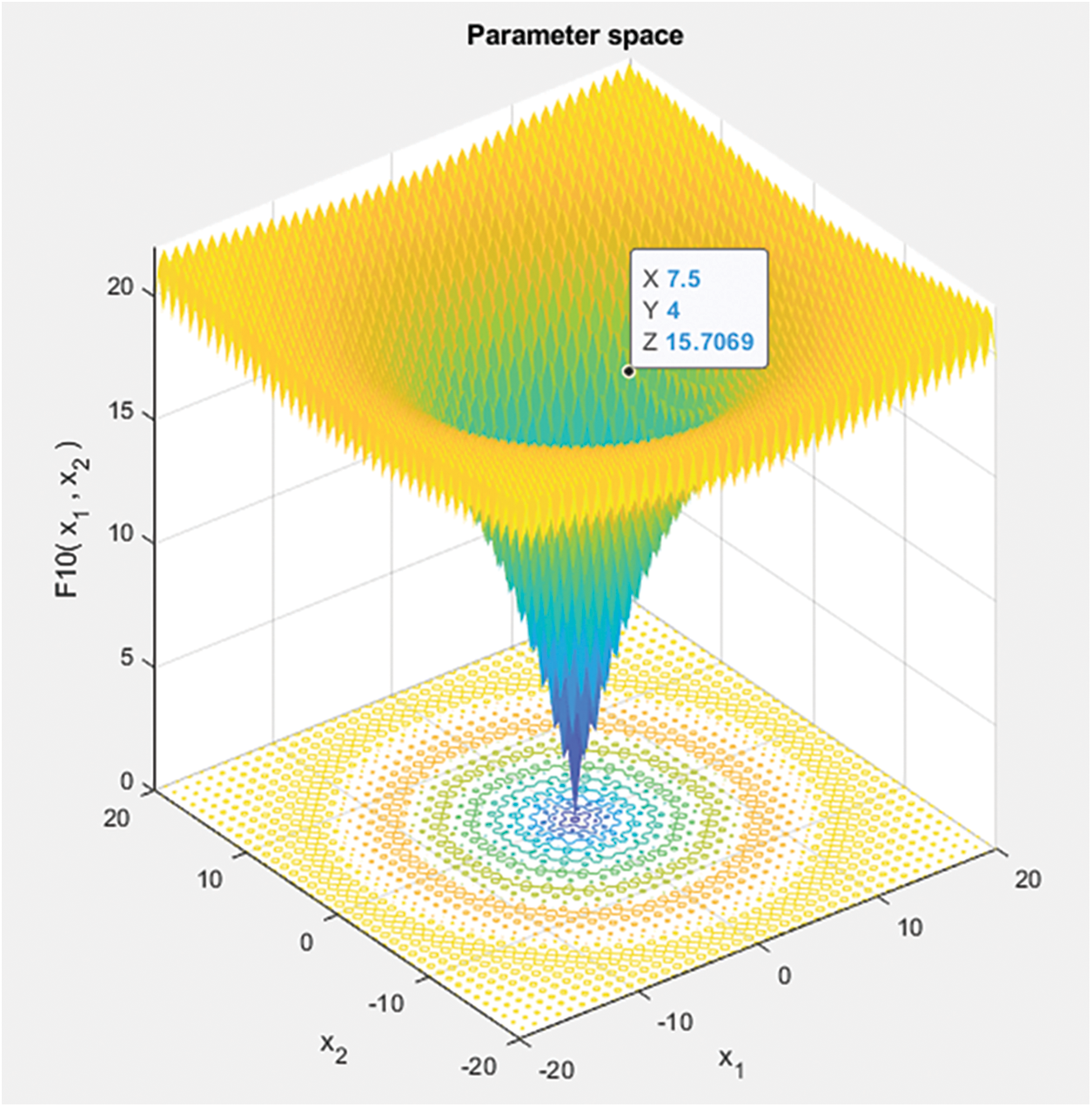
Figure 9: Parametric space of Grey Wolf Optimization

After applying GWO, it can be seen that the models have performed well as shown in Fig. 10 and WSN has also become much more optimized in terms of Packet transfer ratio, Throughput, and End to End delay to make the network more secure, see Table 2 below.

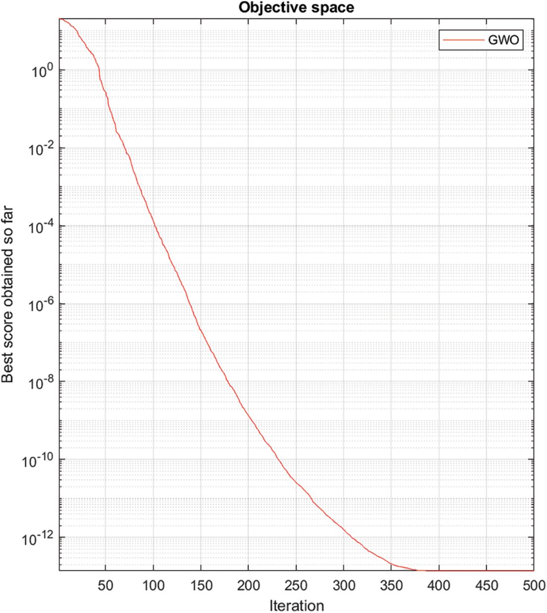
Figure 10: Iterative objective space of Grey Wolf Optimization for securing the network

3.4 Comparative Analysis

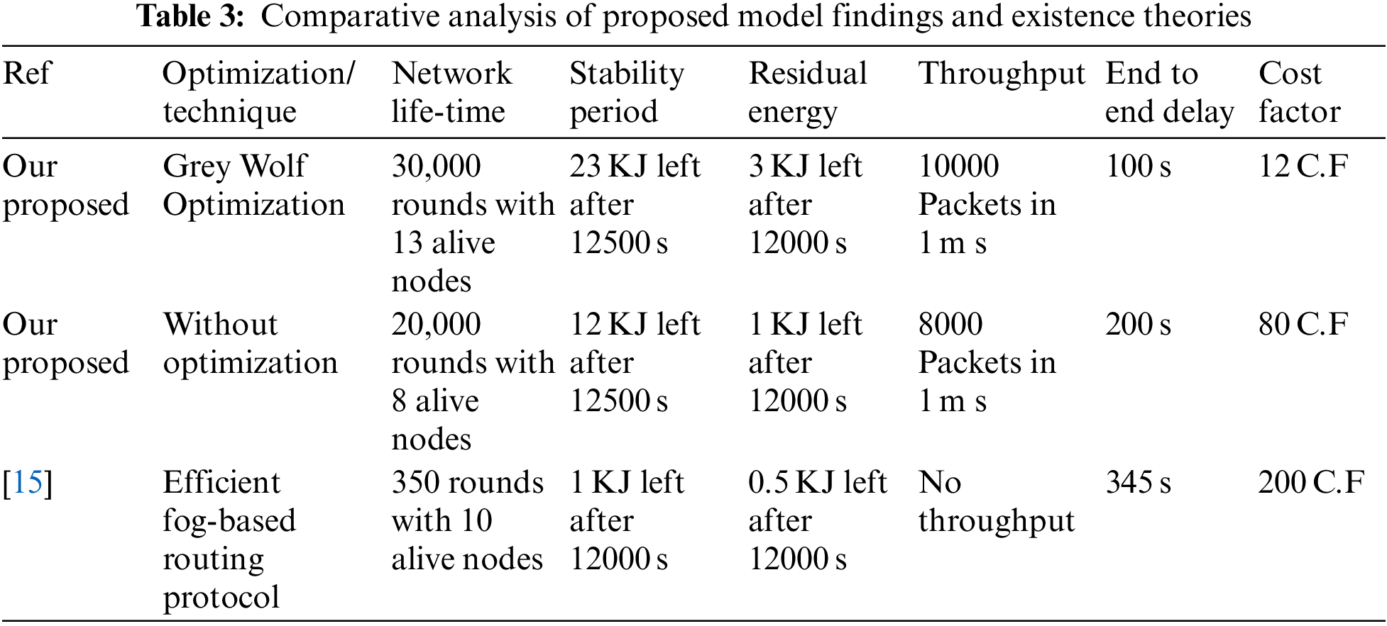
In Table 3, we compared our study with some state-of-the-art research. The placement of sensor nodes on a controlled field can affect the network’s overall performance. The result is a poor cost factor (CF). The formulation’s overall cost factor is computed and optimized by the grey wolf optimization technique to reach the best QoS results.

4  Conclusions and Future Work

Wireless sensor networks are self-configured, and infrastructure networks have fewer resources. Sensor nodes are used to deploy these kinds of networks. Health care, Defense, IoT, smart farming, and many more organizations are used to deploy their networks using WSN. There is no fixed topology and routing mechanism due to the adaptive-algorithms nature of networks. This is also called dynamic routing. Unlike wired networks, wireless networks always face communication issues due to signal fading whenever the environmental conditions are changed. The main emphasis of this study is on improving QoS through a lightweight solution. Various applications require WSNs to meet application-specific performance targets such as efficient routing, minimal overhead, high reliability, throughput and delay, latency rate, and packet transfer ratio. To pursue the required metrics of WSN quality assurance, proposed a novel incorporated lightweight model for QoS improvements. A novel approach is used in this thesis which is integrated with a random waypoint model and grey wolf algorithm. A single algorithm has been implemented. Results show that the hybrid model is more efficient for secure and optimal routing and controlling E-to-E (source-to-destination delay, packet transfer ratio factor. Cost factors show improved results, which is compared with previous studies. Throughput and end-to-end delay due to overhead have been controlled by using RWP’s GWO model. MATLAB and NS2 simulators are used to simulate the results. As previously stated, these areas lead to additional tools (i.e., parameters) that QoS may utilize to balance costs and projected benefits for specific users/clients.

Future Work

We consider that QoS mechanisms will be supplementary operative if users or network tasks can be assigned different levels of security services and requirements, such as response and image allegiance. Security choices can be made within acceptable areas where the service level can indicate security levels in terms of assurance, machine-like strength, administrative strength, and other factors. These domains, as previously shown, lead to additional tools (i.e., parameters) that QoS may use to balance costs and benefits.

Funding Statement: The authors are thankful to the Deanship of Scientific Research at Najran University for funding this work under the Research Collaboration Funding program grant code NU/RC/SERC/11/7.

Conflicts of Interest: The authors declared that they have no conflicts of interest to report regarding the present study.

References

1. K. Haseeb, N. Islam, T. Saba, A. Rehman and Z. Mehmood, “LSDAR: A light-weight structure-based data aggregation routing protocol with secure internet of things integrated next-generation sensor networks,” Sustainable Cities and Society, vol. 54, pp. 101995, 2020. [Google Scholar]
2. M. Ul Hassan, A. Al-Awady, K. Mahmood, S. Ali, I. Algamdi et al., “CNR: A cluster-based solution for connectivity restoration for mobile wsns,” Computers, Materials & Continua, vol. 69, no. 3, pp. 3413–3427, 2021. [Google Scholar]
3. A. Kore and S. Patil, “IC-MADS: IoT enabled cross layer man-in-middle attack detection system for smart healthcare application,” Wireless Personal Communications, vol. 113, no. 2, pp. 727–746, 2020. [Google Scholar]
4. N. Merabtine, D. Djenouri and D. E. Zegour, “Towards energy efficient clustering in wireless sensor networks: A comprehensive review,” IEEE Access, vol. 9, pp. 92688–92705, 2021. [Google Scholar]
5. U. Jain, M. Hussain and J. Kakarla, “Simple, secure, and lightweight mechanism for mutual authentication of nodes in tiny wireless sensor networks,” International Journal of Communication Systems, vol. 33, no. 9, pp. e4384, 2020. [Google Scholar]
6. F. Aliyu, S. Umar and H. Al-Duwaish, “A survey of applications of artificial neural networks in wireless sensor networks,” in 2019 8th Int. Conf. on Modeling Simulation and Applied Optimization (ICMSAO), Manama, Bahrain, IEEE, pp. 1–5, 2019. [Google Scholar]
7. A. Khan and R. Das, “Security aspects of device-to-device (D2D) networks in wireless communication: A comprehensive survey,” Telecommunication Systems, vol. 1, no. 18, pp. 625–642, 2022. [Google Scholar]
8. B. Han, F. Ran, J. Li, L. Yan, H. Shen et al., “A novel adaptive cluster based routing protocol for energy harvesting wireless sensor networks,” Sensors, vol. 22, no. 4, pp. 1564, 2022. [Google Scholar]
9. D. Loganathan, M. Balasubramanian, R. Sabitha and S. Karthik, “Improved load-balanced clustering for energy-aware routing (ILBC-EAR) in WSNs,” Computer Systems Science and Engineering, vol. 44, no. 1, pp. 99–112, 2023. [Google Scholar]
10. M. ul Hassan, K. Mahmood, M. K. Saeed, S. Ali and S. Zaman et al., “Smart node relocation (SNR) and connectivity restoration mechanism for wireless sensor networks,” Wireless Com Network, vol. 1, no. 180, pp. 1–4, 2021. [Google Scholar]
11. S. Rathor and S. Kumari, “Smart agriculture system using IoT and cloud computing,” in 2021 5th Int. Conf. on Information Systems and Computer Networks (ISCON), Mathura, India, IEEE, pp. 1–4, 2021. [Google Scholar]
12. A. P. Pandian, “Development of secure cloud-based storage using the elgamal hyper elliptic curve cryptography with fuzzy logic-based integer selection,” Journal of Soft Computing Paradigm, vol. 2, no. 1, pp. 24–35, 2020. [Google Scholar]
13. M. S. Ali, A. Alqahtani, A. M. Shah, A. Rajab and M. U. Hassan, “Improved-equalized cluster head election routing protocol for wireless sensor networks,” Computer Systems Science and Engineering, vol. 44, no. 1, pp. 845–858, 2023. [Google Scholar]
14. K. Haseeb, I. ud Din, A. Almogren and N. Islam, “An energy efficient and secure IoT-based WSN framework: An application to smart agriculture,” Sensors, vol. 20, no. 7, pp. 2081, 2020. [Google Scholar]
15. R. Fotohi, S. Firoozi Bari and M. Yusefi, “Securing wireless sensor networks against denial-of-sleep attacks using RSA cryptography algorithm and interlock protocol,” International Journal of Communication Systems, vol. 33, no. 4, pp. e4234, 2020. [Google Scholar]
16. M. Ul Hassan, S. Ali, K. Mahmood, M. K. Saeed, A. Al-Awady et al., “An efficient connectivity restoration technique (ecrt) for wireless sensor network,” Computers, Materials & Continua, vol. 69, no. 1, pp. 1003–1019, 2021. [Google Scholar]
17. B. B. Sinha and R. Dhanalakshmi, “Recent advancements and challenges of internet of things in smart agriculture: A survey,” Future Generation Computer Systems, vol. 126, pp. 169–184, 2022. [Google Scholar]
18. K. A. Patil and N. R. Kale, “A model for smart agriculture using IoT,” in 2016 Int. Conf. on Global Trends in Signal processing. Information Computing and Communication (ICGTSPICC), Jalgaon, India, IEEE, pp. 543–545, 2016. [Google Scholar]
19. M. Ali, A. Ali, A. Shah, A. Rajab, M. Hassan et al., “Improved-equalized cluster head election routing protocol for wireless sensornetworks,” Computer Systems Science and Engineering, vol. 44, no. 1, pp. 845–858, 2023. [Google Scholar]
20. K. Haseeb, N. Islam, Y. Javed and U. Tariq, “A lightweight secure and energy-efficient fog-based routing protocol for constraint sensors network,” Energies, vol. 14, no. 1, pp. 89, 2020. [Google Scholar]
21. Y. Liu, Y. Jiang, X. Zhang, Y. Pan and Y. Qi, “Combined grey wolf optimizer algorithm and corrected Gaussian diffusion model in source term estimation,” Processes, vol. 10, no. 7, pp. 1238, 2022. [Google Scholar]
22. A. Norouzi and A. H. Zaim, “Genetic algorithm application in optimization of wireless sensor networks,” The Scientific World Journal, vol. 2014. [Google Scholar]
Cite This Article
Copyright © 2023 The Author(s). Published by Tech Science Press.
This work is licensed under a Creative Commons Attribution 4.0 International License , which permits unrestricted use, distribution, and reproduction in any medium, provided the original work is properly cited.
Downloads
Citation Tools