Computing of LQR Technique for Nonlinear System Using Local Approximation

1  Introduction

The rotary inverted pendulum (RIP) is an unstable system with nonlinear dynamics. RIP is the underactuated mechanical system with lesser control inputs than the degree of freedom. The control of such a system is a more challenging task, and the system becomes a classical benchmark for designing, testing, estimating, and comparing different control techniques [1–5]. The RIP controller design is a crucial problem with the inherent instability feature. Undoubtedly, the RIP has gained importance in the research community in the field of control engineering because of its effectiveness in testing the performance and robustness of different control techniques [6–8]. The objective of the proposed work is contributed in 3 parts: Background Literature Review and Analysis; Proposed Work and Novelty Aspects; Experimental Results.

1.1 Background Literature Review and Analysis

It is a multivariable nonlinear dynamical system having two links. One link revolves around an axis in the horizontal plane so that the other can balance itself upright [9,10]. Due to its nonlinear behaviour, the RIP control helps design the altitude controller of rockets and satellites. RIP control plays a vital role in real-life applications ranging from robotics to aerospace, locomotive to marine systems, and flexible to pointing control systems. Additionally, studying the dynamics and control of an inverted pendulum helps maintain the equilibrium of tall buildings [11–15].

Model-based control techniques have been used frequently, but fuzzy and non-model-based approaches have been utilized too. Newton’s laws or energy balance approaches have been used to formulate the dynamic model [16–19]. The fuzzy cascade control based on Hierarchical Fair Competition-based Genetic Algorithms has been used in [20]. The fuzzy cascade control approach has been designed as a nonlinear system with higher disturbance and settling time. It consists of two fuzzy controllers placed in a cascade manner, and their parameters are optimized using a genetic algorithm. The inner loop controls the position of the rotating arm, while the outer loop provides the appropriate input to the inner loop due to a change in the angle of the vertical arm. Simulation has been performed, and the results have been validated on the real hardware. The counter-based approach has been used to design swings, while pole placement with an integrator has been used to stabilize the vertical arm [21]. The study shows a settling time of 4.5 s for the swing-up controller. Similarly, stabilization of the vertical arm has been shown through simulation.

The energy-based method achieves swing-up and vertical stabilization [22]. The H2 / H∞ has been used to reduce oscillations and stabilize the system. Compared to the feedback controller, fewer oscillations have been observed with the proposed controller. The only drawback is the control signal is not optimal and requires a higher value for smaller fluctuations. Kharitonov polynomial has been formed with a proportional-integral (PI) controller transfer function [23]. Routh Hurwitz criteria have been utilized to design a stable controller, and stability has been analyzed using the Nyquist plot. A swing-up controller has been designed in [24]. It is based on energy control and feedback linearization. Simulation has been performed to show the effectiveness of the proposed approach. The value of gain has been associated with energy convergence to zero. The higher gain means faster convergence. Another control approach has been reported in [25]. It consists of a backstepping controller for swing-up and linear state feedback controllers for stabilization. The quadratic Lyapunov system and Sylvester’s criterion have been used to determine a sufficient stability margin around the equilibrium point. A comparison has been developed between the proposed method and the classical scheme. The results have been evaluated in percentage to show the effectiveness of the proposed approach.

1.2 Proposed Work and Novelty Aspects

Fig. 1 depicts the rotary inverted pendulum module coupled to the Quanser SRV02 plant in the correct configuration. SRV02 has a direct current (DC) motor enclosed in an aluminum frame and is equipped with a planetary gearbox. The module is attached to the SRV02 load gear, and the pendulum arm is linked to the module body. The linear quadratic regulator (LQR) has been designed to stabilize the pendulum. The LQR is an excellent approach that provides optimal feedback to make a closed-loop system robust and stable. It also provides a local approximation to develop optimal control for nonlinear systems [26].

Figure 1: Rotary inverted pendulum

To our knowledge, no efforts have been reported in the literature so far in which an optimal controller for a nonlinear system such as a rotatory inverted pendulum has been designed and implemented using Newton-Euler, Lagrange method, and local approximation. In the current research work, the following are the key contributions:

•   The system has been modelled.

•   The resulting model has been linearized around an equilibrium point.

•   The comparison of the two models has been made in Matlab and Simulink to find the local approximation.

•   The linearized state-space model has been used to estimate the parameters of the LQR controller.

•   The controller has been implemented for both models, and its performance and stability have been analyzed.

1.3 Experimental Results

The proposed work has been implemented, and the hardware is developed, as shown in Fig. 1. From the experimental results, it is seen that theoretical results are well verified from the experimental results.

The paper is organized as follows. In Section 2, mathematical modelling has been developed, and linearization has been done around the equilibrium point. The simulation result of the comparison to find a local approximation has been described in Section 3. The controller design has been discussed in Section 4. Section 5 highlights the performance and stability of the controller. The conclusion of the paper has been given in Section 6.

2  System Model Development

The Lagrange method has been used to develop the mathematical model of this underactuated nonlinear unstable system Newton-Euler. Newton-Euler equations describe the translation and rotation of a rigid body. These equations show the relation among forces and torques acting on a rigid body in the form of matrices [27]. Lagrange establishes the relationship between the net energy of the system and forces or torques acting on it through partial differentiation. Thus, it becomes convenient to develop a mathematical model of the system using its potential and kinetic energy [28].

A free-body diagram of RIP mounted on a box having the reference frames is presented in Fig. 2. The horizontal link with length r is rotating with an angle θ, and the vertical arm of length L and mass m swings with an angle α . Reference frames have been attached to the moving links for the calculation of the position vector ( P_ ) with respect to a fixed frame. All the symbols used in the mathematical modelling are given in Table 1.

Figure 2: Free body diagram of the pendulum with reference frames

2.1 Design Parameters

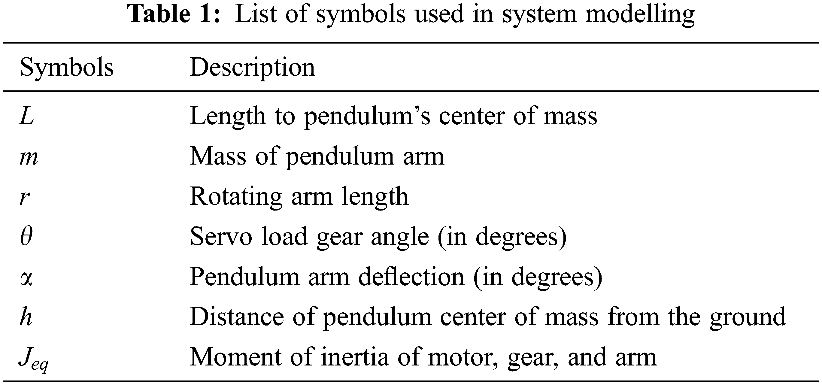
The potential energy (PE) Ep of the inverted pendulum is given by [29]:

Ep=mgLcosα (1)

where m is the mass of the pendulum arm, g denotes the force of gravity, L represents the length of the pendulum’s center of mass, and α is the deflection of the pendulum arm. The kinetic energy (KE) Ek of the inverted pendulum is given by [30]:

Ek=mv22+Jeqθ˙22 (2)

v2=r2θ˙2+L2sin2αθ˙2+L2α˙2−2rLcosαθ˙α˙ (3)

Substituting Eqs. (3) in (2), we get

Ek=12mr2θ˙2+12mL2sin2αθ˙2+12mL2α˙2−mrLcosαθ˙α˙+Jeqθ˙22 (4)

The Lagrangian LLagr is given by:

LLagr=Ek−Ep (5)

LLagr=12mr2θ˙2+12mL2sin2(α)θ˙2+12mL2α˙2−mrlcosαθ˙α˙+12Jeqθ˙2−mgLcosα (6)

Now by simplification of Eq. (A21) from Appendix A.1, we got the following results:

θ¨=1(sin2α.(L2+r2)+Jeqm)[Tm−2L2sinαcosαθ˙α˙−rLsinαα˙2+rLsinαcos2αθ˙2+rgcosαsinα] (7)

Substituting the value θ¨ in Eq. (A19) in Appendix A.1:

α¨=(rcosαL[sin2α(L2+r2)+Jeqm])[Tm−2L2sinαcosαθ˙α−rLsinαα˙2+rLsinαcos2αθ˙2+rgcosαsinα]+sinαcosαθ˙2+gLsinα (8)

2.2 Linearization Around an Equilibrium Point

Mathematical modelling uses the Newton-Euler, Lagrange method to design a controller. The resulting model was nonlinear, so linearization was required, which was done around an equilibrium point. Following are the assumptions from Eqs. (7) and (8):

θ¨=(1sin2α(L2+r2)+Jeqm)[Tm−L2sin2αθ˙α˙−rLsinαα˙2+rLsinαcos2αθ˙2+12rgcosαsin2α] (9)

α¨=(rcosαLsin2α(L2+r2)+Jeqm)[ Tm−L2sin2αθ˙α˙−rLsinαα˙2+rLsinαcos2αθ˙2+12rgsin2α ]++gLsinα (10)

where θ¨=f1 and α¨=f2 . The linearized system is given by (see derivation in Appendix A.2):

[θ˙θ¨α˙α¨]=[010000mrgJeq0000100gL(1+mr2Jeq)0][θθ˙αα˙]+[01Jeq0rLJeq]T (11)

[y1y2]=[10000010][θθ˙αα˙] (12)

The motor torque is given by:

T=Tgear−Beqθ˙=KtKgRmηmηg(U−KmKgθ˙)−Beqθ˙=KtKgRmηmηgU−θ˙(KtKg2KmRmηmηg+Beq) (13)

where U is the input voltage and is a control signal. Substitute the value of T in the state-space model, and we get:

[θ˙θ¨α˙α¨]=[010000mrgJeq0000100gL(1+mr2Jeq)0][θθ˙αα˙]+[0KtKgηmηgRmJeq0rKtKgηmηgLRmJeq]U−[0a0b].θ˙ (14)

where:

a=−1Jeq(KtKg2KmηmηgRm+Beq)

b=−rLJeq(KtKg2KmηmηgRm+Beq)

[θ˙θ¨α˙α¨]=[01000am.r.gJeq000010bgL(1+mr2Jeq)0][θθ˙αα˙]+[0KtKgηmηgRmJeq0rKtKgηmηgLRmJeq]U (15)

where, Beq denotes the viscous damping of the motor, ηg is the efficiency of the gear, ηm represents the efficiency of the motor, Rm is the resistance of the motor, Kt is the torque constant of the motor, Kg is the gear ratio, Km is the damping constant, Kenc is the encoder constant, and U is the control voltage.

3  Estimation of Local Approximation for Nonlinear System

To find the range of angle ( α ) for which a nonlinear model behaves linearly around an equilibrium point, i.e., local approximation, to develop optimal control of a nonlinear system, a comparison of linear and nonlinear models has been performed in MATLAB Simulink and the setup is shown in Fig. 3. Comparison has been made by setting the initial value of 1∘ of α in both models without any input. The vertical arm will start falling under the influence of gravity. The value of angle α will begin rising. The result of the comparison is given in Fig. 4. It can be seen that the variation in α is the same until 20∘ for both models, and the difference is 0∘ . After that nonlinear model behaves differently, and the angle difference starts rising. It has given an excellent local approximation, and control must be done in this range, i.e., from −20∘ to 20∘ . The controller has been designed with a much smaller range than the estimated range.

Figure 3: System setup for the local approximation evaluation

Figure 4: Comparison of variation in α for the linear and nonlinear system

4  Controller Design and Parameters Estimation

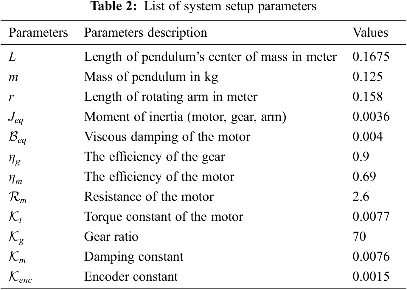
MATLAB (2018a, MathWorks, MA, USA) has been used to evaluate the parameters of the LQR controller. Matrices A and B have been assessed using the system setup parameters and initial conditions in Table 2. These parameters are for rotary inverted pendulum hardware developed by Quanser. Q matrix has weights on the states of the system. Similarly, controller vector K has been evaluated using the same parameters and MATLAB LQR function.

A=[01000−20.3854.06000010−19.22109.560]

B=[035.84033.81]

Q=[1000010000100001]

Q matrix contains 1 in the main diagonal, which means the angular velocities, i.e., ( θ˙ , α˙ ) have also been considered in the evaluation.

K=[−1−2.0227.683.56]

5  Controller Validation

The designed controller has been simulated in Matlab Simulink. Simulation has been performed for both models, and the controller’s performance has been presented in this section. The plots show the variation in angles along the vertical axis vs. time along the horizontal axis. These plots have been generated by varying θ and α . Results have been presented first for the linear system and then for the nonlinear system.

5.1 Linear System

Fig. 5 shows the simulation setup for the linear model along with an LQR Controller in Simulink. Fig. 6 shows the performance and stable behaviour of the RIP. Both angles are zero at the beginning of the simulation. Then, the RIP was disturbed by rotating θ at 5.7∘ (0.1 rad) after 5 s. The vertical arm swings at an angle of approximately 0.19∘ due to the horizontal link’s motion and returning to its initial stable position, i.e., it stays upright. The variation in angle α due to the change in θ has been adjusted by the controller as shown in Fig. 6. The system is stable at the new orientation of θ, and the vertical arm is still maintaining zero inclination, i.e., it is not falling in any direction rightward or leftward.

Figure 5: Simulation of a linear model with a controller in MATLAB simulink

Figure 6: Stability analysis by varying the θ

Similarly, the vertical arm of RIP has been shaken by setting α5.7∘ (0.1 rad) at the beginning as the initial condition, as shown in Fig. 7. The controller rotates the horizontal link from zero to approximately −13∘ to balance the vertical arm and brings it to its stable upright position. θ angle has been brought back to zero in 5 s. It shows that the controller adjusts the variation in both variables of the system and maintains the vertical arms in a stable upright position. The presentation of the results validates the designed controller.

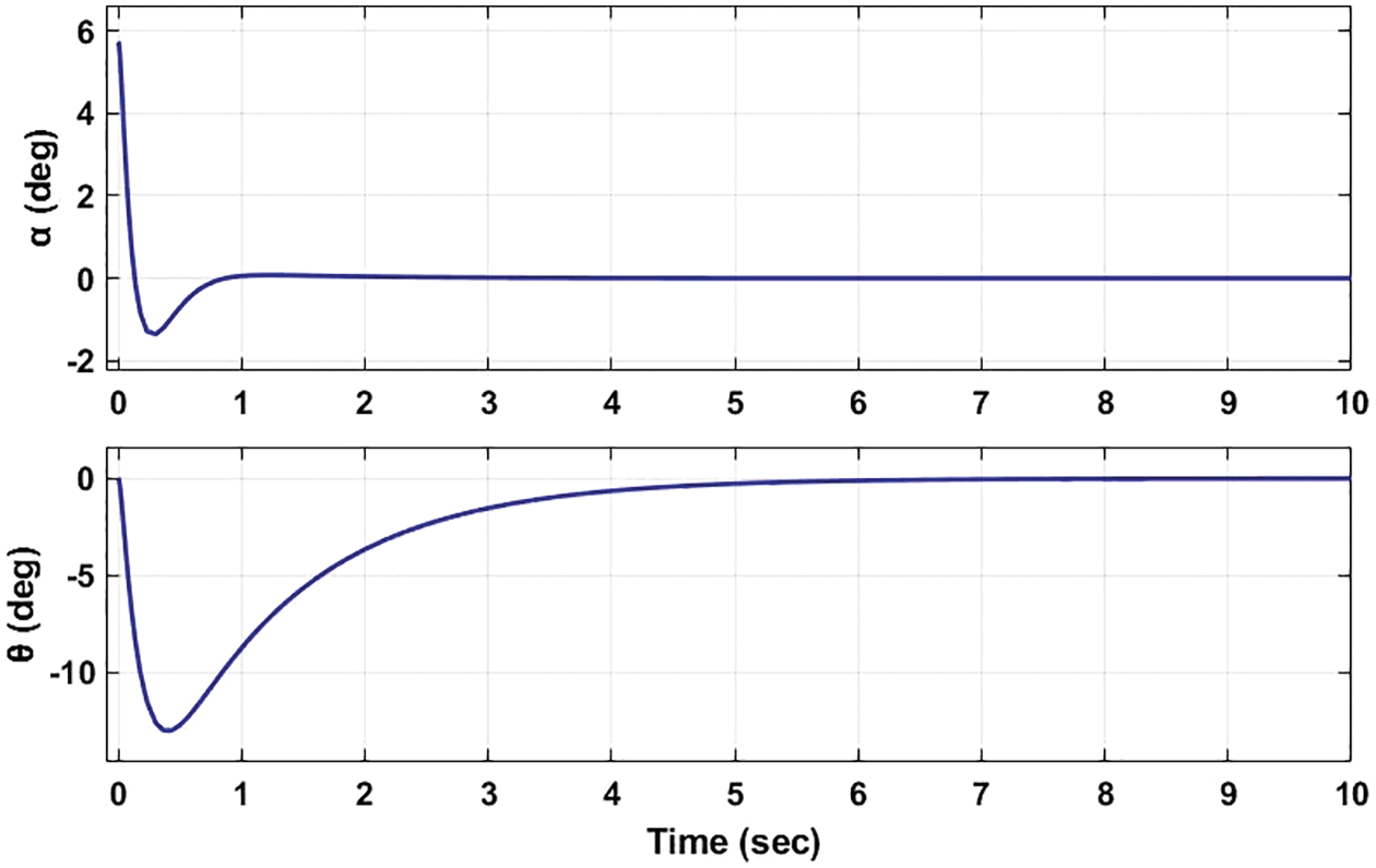
Figure 7: Stability analysis by varying the α

5.2 Nonlinear System

Fig. 8 shows the simulation setup for the nonlinear model along with LQR Controller. The performance of the LQR has also been tested on the nonlinear model because it provides a local approximation to develop an optimal controller for nonlinear systems.

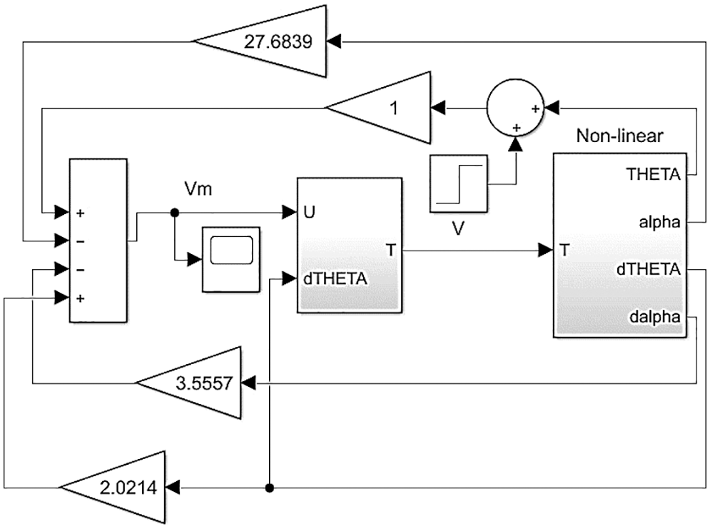
Figure 8: Simulation of a nonlinear model with a controller in MATLAB simulink

In Fig. 9 θ has been moved from 0∘ to 5.7∘ for initial five seconds, and then it has been rotated back to 0∘ . The vertical arm’s angle α has swung twice, but the controller has brought it back to its stable vertical position, as shown in Fig. 9.

Figure 9: Variation in θ for the nonlinear system

Similarly, the performance of the controller has been evaluated by changing both variables of the system, i.e., ( θ and α ), as shown in Fig. 10. In the beginning, the controller adjusts the α to 0∘ , which was given an initial value of 5.7∘ (0.1 rad). The corresponding rotation of θ is shown in Fig. 10. After 5 s, the θ has been set at 5.7∘ (0.1 rad) α has been brought back to 0∘ by the controller.

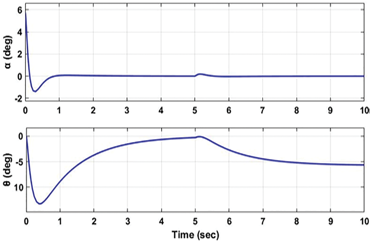
Figure 10: Variation in α for the nonlinear system

6  Hardware Implementation and Analysis

The designed controller has been tested over an inverted pendulum, shown in Fig. 1, and the results are shown in Figs. 11 and 12. These plots depict the comparison in a real and simulated environment. Fig. 12 shows the variation in angle θ, and Fig. 11 shows the corresponding angle α . The blue line with dots represents the measured value, and the green is of simulation results. It is vivid from that the actual measured values are very close to the simulated values. These results validate the proposed controller. The controller adjusted the disturbance and kept the pendulum in a stable upright position, as shown in Fig. 11, by rotating the horizontal link of the pendulum.

Figure 11: Pendulum arm deflection α

Figure 12: Servo load gear angle θ

7  Conclusion & FutureWork

In the proposed research work, we have designed a state-feedback controller for the inverted rotary pendulum utilizing the LQR techniques. A complete set of analyses has been developed to provide a validation of the designed system. The performance of the designed controller is measured for the linear and the nonlinear system using the local approximation. It is evident from the simulation results that the designed controller is giving optimal performance and is robust enough to keep the pendulum in an upright, stable position. The performance has been evaluated by varying the angles of the horizontal and vertical arms of the RIP. From the simulation results, it can be seen that the controller stabilizes the pendulum arm under various disturbances in a specific range. The simulation results have been validated over a real, inverted pendulum. In future, a fuzzy controller will be implemented to compare the performance of the two controllers.

Acknowledgement: Authors would like to thank Christopher Hille and Dmitry Konstantinov for a thorough discussion.

Funding Statement: The authors received no specific funding for this study.

Conflicts of Interest: The authors declare they have no conflicts of interest to report regarding the present study.

Appendix

Appendix A

A.1 Derivation of θ¨andα¨

To evaluate v, a position vector P_ of mass must be defined as,

P_=[xyz]=[cosθ−sinθ0sinθcosθ0001]([r00]+[1000cosαsinα0−sinαcosα][00−L]) (A1)

P_=[xyz]=[cosθ−sinθ0sinθcosθ0001][r−Lsinα−Lcosα] (A2)

P_=[xyz]=[rcosθ+Lsinθsinαrsinθ+Lcosθsinα−Lcosα] (A3)

where r denotes the length of the horizontal link. To evaluate v, we need to differentiate the position vector P_ of m as,

v_=P_=[x˙y˙z˙]=[−rsinθθ˙+Lcosθsinαθ˙+Lsinθcosαα˙−rcosθθ˙+Lsinθsinαθ˙−Lcosθcosαα˙−Lsinαα˙] (A4)

v2=x˙2+y˙2+z˙2=(−rsinθθ˙+Lcosθsinαθ˙+Lsinθcosαα˙)2+(−rcosθθ˙+Lsinθsinαθ˙−Lcosθcosαα˙)2+(−Lsinαα˙)2 (A5)

v2=r2θ˙2+L2sin2αθ˙2+L2cos2αα˙2−2rLcosαθ˙α˙+L2sin2αα˙2 (A6)

Taking the differential of Eq. (6) with respect to θ˙ to get,

δδθ˙[LLagr]=mr2θ˙+mL2sin2αθ˙−mrLcosαα˙+Jeqθ˙ (A7)

Now taking d/dt of Eq. (A7) to get:

ddt(δδθ˙[ ℒLagr ])=mr2θ¨+2mL2sinαcosαθ˙α˙+mL2sin2αθ¨+mrLsinαα˙2−mrLcosαα¨+Jeqθ¨  (A8)

Taking the differential of Eq. (6) with respect to θ to get:

δδθ[LLagr]=0 (A9)

where:

ddt(δδθ˙[LLagr])−δδθ[LLagr]=T (A10)

where T denotes the torque. By inserting Eqs. (A8) and (A9) in (A10) to get:

mr2θ¨+2mL2sinαcosαθ˙α˙+mL2sin2αθ¨+mrLsinαα˙2−mrLcosαα¨+Jeqθ¨=T (A11)

Now differentiating Eq. (6) with respect to α and α˙ respectively to get:

δδα[LLagr]=mL2sinαcosαθ˙2+mrLsinαθ˙α˙+mgLsinα (A12)

δδα˙[LLagr]=mL2α˙−mrLcosαθ˙ (A13)

Now taking ddt of Eq. (A18) to get:

ddt(δδα˙[LLagr])=mL2α¨+mrLsinαθ˙α˙−mrLcosαθ¨ (A14)

where:

ddt(δδα˙[LLagr])−δδα[LLagr]=0 (A15)

Now simplify Eq. (A15) to get:

mL2α¨−mrLcosαθ¨−mL2sinαcosαθ˙2−mgLsinα=0 (A16)

Finally, we get two equations (i.e., Eqs. (A17) and (A18)) of the system as below:

r2θ¨+2L2sinαcosαθ˙α˙+L2sin2αθ¨+rLsinαα˙2−rLcosαα¨+Jeqmθ¨=Tm (A17)

Lα¨−rcosαθ¨−Lsinαcosαθ˙2−gsinα=0 (A18)

From Eq. (A18), the value of α¨ is obtained as:

α¨=rLcosαθ¨+sinαcosαθ˙2+gLsinα (A19)

Substituting the value of α¨ from Eqs. (A19) in (A17)

r2θ¨+2L2sinαcosαθ˙α˙+L2sin2αθ¨+rLsinαα˙2−r2cos2αθ¨−rLsinαcos2αθ˙2−rgcosαsinα+Jeqmθ¨=Tm (A20)

Now simplifying Eq. (A20):

θ¨[sin2α(L2+r2)+Jeqm]+2L2sinαcosαθ˙α˙+rLsinαα˙2−rLsinαcos2αθ˙2−rgcosαsinα=Tm (A21)

A.2 System Linearization

The linear system can be expressed by:

x˙_=A_x_+B_u_,y_=C_x_+D_u_ (A22)

For the nonlinear system, the linearized system looks as follows:

[θ˙θ¨α˙α¨]=[0100δf1δθx_=xo_δf1δθ˙x_=xo_δf1δαx_=xo_δf1δα˙x_=xo_0001δf2δθx_=xo_δf2δθ˙x_=xo_δf2δαx_=xo_δf2δα˙x_=xo_][θθ˙αα˙]+[0δf1δTx_=xo_0δf2δTx_=xo_]T (A23)

[y1y2]=[10000010][θθ˙αα˙] (A24)

The equilibrium point is given by:

xo_=[θo000];δδθ[f1]=0;δδθx_=xo_[f1]=0;δδθ˙x_=xo_[f1]=0 (A25)

δδθ˙[f1]=(1sin2α(L2+r2)+Jeqm)[−L2sin2αα˙+2rLsinαcos2αθ˙] (A26)

δδα[f1]=(−2sinαcosα(L2+r2)[sin2α(L2+r2)+Jeqm]2)×[Tm−L2sin2αθ˙α˙−rLsinαα˙2+rLsinαcos2αθ˙2+12rgsin2α]+(1sin2α(L2+r2)+Jeqm)×[−2L2cos2αθ˙α˙−rLcosαα˙2+rLcos3αθ˙2−2rLsin2αcosαθ˙2+rgcos2α] (A27)

δδαx_=xo_[f1]=mrgJeq;δδα˙x_=xo_[f1]=0 (A28)

δδα˙[f1]=(1sin2α(L2+r2)+Jeqm)[−L2sin2αθ˙−2rLsinαα˙] (A29)

δδT[f1]=(1sin2α(L2+r2)+Jeqm)1m (A30)

δδTx_=xo_[f1]=1Jeq;δδθ[f2]=0;δδθx_=xo_[f2]=0;δδθ˙x_=xo_[f2]=0 (A31)

δδθ˙[f2]=(rcosαL[sin2α(L2+r2)+Jeqm])[−L2sin2αα˙+2rLsinαcos2αθ˙] (A32)

δδα[f2]=(−Lrsinα(sin2α(L2+r2)+Jeqm)[L(sin2α(L2+r2)+Jeqm)]2)−(2Lrsinαcos2α(L2+r2)[L(sin2α(L2+r2)+Jeqm)]2)[Tm−L2sin2αθ˙α˙−rLsinαα˙2+rLsinαcos2αθ˙2+12rgsin2α]+(rcosαL(sin2α(L2+r2)+Jeqm))[−2L2cos2αθ˙α˙−rLcosαα˙2+rLcos3αθ˙2−2rLsin2αcosαθ˙2+rgcos2α]+cos2αθ˙2+gLcosα (A33)

δδαx_=xo_[f2]=mr2gJeqL+gL;δδα˙x_=xo_[f2]=0; (A34)

δδTx_=xo_[f2]=rLJeq (A35)

δδα˙[f2]=(rcosαL[sin2α(L2+r2)+Jeqm])[−L2sin2αθ˙−2rLsinαα˙] (A36)

δδT[f2]=(rcosαL[sin2α(L2+r2)+Jeqm])1m (A37)

References

1. A. Shahzad, Aamir, S. Munshi, S. Azam and M. N. Khan, “Design and implementation of a state-feedback controller using LQR technique,” CMC-Computers Materials & Continua, vol. 73, no. 2, pp. 2897–2911, 2022. [Google Scholar]
2. N. Arulmozhi and T. A. A. Victorie, “Kalman filter and H-infinity filter based linear quadratic regulator for furuta pendulum,” Computer Systems Science and Engineering, vol. 43, no. 2, pp. 605–623, 2022. [Google Scholar]
3. Z. Meng, Z. Hu, Z. Ai, Y. Zhang and K. Shan, “Research on planar double compound pendulum based on RK-8 algorithm,” Journal on Big Data, vol. 3, no. 1, pp. 11–20, 2021. [Google Scholar]
4. N. P. Nguyen, H. Oh, Y. Kim and J. Moon, “A nonlinear hybrid controller for swinging-up and stabilizing the rotary inverted pendulum,” Nonlinear Dynamics, vol. 104, no. 1, pp. 1117–1137, 2021. [Google Scholar]
5. A. de. Carvalho, J. F. Justo, B. A. Angélico, A. M. de. Oliveira and J. I. da. S. Filho, “Rotary inverted pendulum identification for control by paraconsistent neural network,” IEEE Access, vol. 9, no. 1, pp. 74155–74167, 2021. [Google Scholar]
6. Y. Dai, K. Lee and S. Lee, “A real-time HIL control system on rotary inverted pendulum hardware platform based on double deep Q-network,” Measurement and Control, vol. 54, no. 3–4, pp. 417–428, 2021. [Google Scholar]
7. H. -R. Li, Z. -Y. Nie, E. -Z. Zhu, W. -X. He and Y. -M. Zheng, “Double loop DR-PID control of a rotary inverted pendulum,” in Proc. IEEE Int. Conf. on Networking, Sensing and Control (ICNSC), Xiamen, China, pp. 1–5, 2021. [Google Scholar]
8. Z. S. Mahmood, I. B. Kadhim and A. N. Nasret, “Design of rotary inverted pendulum swinging-up and stabilizing,” Periodicals of Engineering and Natural Sciences, vol. 9, no. 4, pp. 913–920, 2021. [Google Scholar]
9. J. Huang, T. Zhang, Y. Fan and J. -Q. Sun, “Control of rotary inverted pendulum using model-free backstepping technique,” IEEE Access, vol. 7, no. 1, pp. 96965–96973, 2019. [Google Scholar]
10. M. F. Hamza, H. J. Yap, I. A. Choudhury, A. I. Isa, A. Y. Zimit et al., “Current development on using rotary inverted pendulum as a benchmark for testing linear and nonlinear control algorithms,” Mechanical Systems and Signal Processing, vol. 116, no. 1, pp. 347–369, 2019. [Google Scholar]
11. M. Antonio-Cruz, R. Silva-Ortigoza, J. Sandoval-Gutiérrez, C. A. Merlo-Zapata, H. Taud et al., “Modeling, simulation, and construction of a furuta pendulum test-bed,” in Proc. Int. Conf. on Electronics, Communications and Computers (CONIELECOMP), Cholula, Mexico, pp. 72–79, 2015. [Google Scholar]
12. Y. -F. Chen and A. -C. Huang, “Adaptive control of rotary inverted pendulum system with time-varying uncertainties,” Nonlinear Dynamics, vol. 76, no. 1, pp. 95–102, 2014. [Google Scholar]
13. S. Jadlovský and J. Sarnovský, “Modelling of classical and rotary inverted pendulum systems-A generalized approach,” Journal of Electrical Engineering, vol. 64, no. 1, pp. 12–19, 2013. [Google Scholar]
14. N. J. Mathew, K. K. Rao and N. Sivakumaran, “Swing up and stabilization control of a rotary inverted pendulum,” IFAC Proceedings Volumes, vol. 46, no. 32, pp. 654–659, 2013. [Google Scholar]
15. P. Seman, B. Rohal-Ilkiv, M. Juh and M. Salaj, “Swinging up the furuta pendulum and its stabilization via model predictive control,” Journal of Electrical Engineering, vol. 64, no. 3, pp. 152–158, 2013. [Google Scholar]
16. I. Hassanzadeh and M. Saleh, “Controller design for rotary inverted pendulum system using evolutionary algorithms,” Mathematical Problems in Engineering, vol. 2011, no. 1, pp. 1–17, 2011. [Google Scholar]
17. T. C. Kuo, Y. J. Huang and B. W. Hong, “Adaptive PID with sliding mode control for the rotary inverted pendulum system,” in Proc. IEEE/ASME Int. Conf. on Advanced Intelligent Mechatronics, Singapore, pp. 1804–1809, 2009. [Google Scholar]
18. D. I. Barbosa, J. S. Castillo and L. F. Combita, “Rotary inverted pendulum with real time control,” in Proc. IX Latin American Robotics Symp. and IEEE Colombian Conf. on Automatic Control, Bogota, Colombia, pp. 1–6, 2011. [Google Scholar]
19. M. Akhtaruzzaman and A. A. Shafie, “Modeling and control of a rotary inverted pendulum using various methods, comparative assessment and result analysis,” in Proc. IEEE Int. Conf. on Mechatronics and Automation, Xi’an, China, pp. 1342–1347, 2010. [Google Scholar]
20. S. -K. Oh, S. -H. Jung and W. Pedrycz, “Design of optimized fuzzy cascade controllers by means of hierarchical fair competition-based genetic algorithms,” Expert Systems with Applications, vol. 36, no. 9, pp. 11641–11651, 2009. [Google Scholar]
21. V. Nath and R. Mitra, “Swing-up and control of rotary inverted pendulum using pole placement with integrator,” in Proc. IEEE Recent Advances in Engineering and Computational Sciences (RAECS), Chandigarh, India, pp. 1–5, 2014. [Google Scholar]
22. Al-Jodah, H. Zargarzadeh and M. K. Abbas, “Experimental verification and comparison of different stabilizing controllers for a rotary inverted pendulum,” in Proc. IEEE Int. Conf. on Control System, Computing and Engineering, Penang, Malaysia, pp. 417–423, 2013. [Google Scholar]
23. J. George, B. Krishna, V. George, C. Shreesha and M. K. Menon, “Stability analysis and design of pi controller using kharitnov polynomial for rotary inverted pendulum,” Sensors & Transducers Journal, vol. 138, no. 3, pp. 104–113, 2012. [Google Scholar]
24. K. Chou and Y. Chen, “Energy based swing-up controller design using phase plane method for rotary inverted pendulum,” in Proc. 13th IEEE Int. Conf. on Control Automation Robotics & Vision (ICARCV), Singapore, pp. 975–979, 2014. [Google Scholar]
25. A. Tiga, C. Ghorbel and N. B. Braiek, “Nonlinear/linear switched control of inverted pendulum system: Stability analysis and real-time implementation,” Mathematical Problems in Engineering, vol. 2019, no. 1, pp. 1–10, 2019. [Google Scholar]
26. L. Wei and W. Yao, “Design and implement of LQR controller for a self-balancing unicycle robot,” in Proc. IEEE Int. Conf. on Information and Automation, Lijiang, China, pp. 169–173, 2015. [Google Scholar]
27. V. Aslanov, G. Kruglov and V. Yudintsev, “Newton–Euler equations of multibody systems with changing structures for space applications,” Acta Astronautica, vol. 68, no. 11–12, pp. 2080–2087, 2011. [Google Scholar]
28. J. M. Mazón, “The Euler–Lagrange equation for the anisotropic least gradient problem,” Nonlinear Analysis: Real World Applications, vol. 31, no. 1, pp. 452–472, 2016. [Google Scholar]
29. Y. Silik and Y. Ulas, “Control of rotary inverted pendulum by using on–off type of cold gas thrusters,” Actuators, vol. 9, no. 4, pp. 1–17, 2020. [Google Scholar]
30. N. Gupta and L. Dewan, “Modeling and simulation of rotary-rotary planer inverted pendulum,” Journal of Physics: Conference Series, vol. 1240, no. 1, pp. 1–9, 2019. [Google Scholar]
Appendix
Appendix A
A.1 Derivation of
To evaluate v, a position vector