A Deep Learning Ensemble Method for Forecasting Daily Crude Oil Price Based on Snapshot Ensemble of Transformer Model

1  Introduction

Due to the widespread use of oil in many economic sectors, it is considered one of the world’s most potential sources of energy [1]. The economic development of a country can be driven or hindered based on its consumption and production [2]. Oil is a key factor in driving the global economy forward. It is still the main origin of energy, responsible for the creation of about a third of worldwide energy. Because oil prices are volatile, economy experts exert tremendous efforts to reach a better understanding of how oil price affects the global economy and the global financial market mechanics. As a result, price volatility leads to increased inflation and a decrease in cumulative demand [3].

In the energy market, the global economy heavily relies on energy consumption, As the fluctuation in oil prices could disrupt important economic domains such as industry and supply chains. On one hand, the surge in oil demand could lead to slowing the growth of oil importing countries. In addition, it benefits exporting countries [4]. While it is commonly agreed that a surge in oil prices affects all other goods since it is the main driver of transportation. Thus, a well-established prediction of oil prices has become a significant subject that has gained attention from all government agencies as it would aid policymakers adopt convenient policies and take a proper decision considering natural energy resources. Furthermore, studies show that oil prices have a notable impression on other financial markets [5].

Controlling major oilfields requires quick decisions while addressing ongoing issues. The Smart Oilfield will help with the digitization of instrumentation systems and the development of network-based knowledge exchange in order to optimize production processes [6,7]. Hence, ablility to forecast the prospective crude oil price has been a remarkable issue in the forecasting research field [8]. Crude oil price forecasting is beneficial in obtaining a greater comprehension of the global economic state [9]. Despite the vast literature on the implications of speculation on the price of oil, no consensus has been reached [10]. However, many researchers have successfully predicted oil prices using various methods [11]. In the energy market, oil price forecasting is seen as a challenging task [12].

Generally, forecasting methods can be grouped into three clusters. The first cluster includes statistical models such as random walk (RW) [13], generalized auto regressive conditional heteroskedasticity (GARCH) family models [14], autoregressive integrated moving average (ARIMA) models [15], error correction models (ECM) [16], etc. The second cluster is concerned with models that originate from expert systems and artificial intelligence (AI) such as support vector machine (SVM) [17], adaptive neuro-fuzzy inference system (ANFIS) [18], neural network and deep learning model [19].

Conventional statistical and econometric approaches have the ability to capture linear patterns in time series data. Such methods may be unsatisfactory to reveal the nonlinear features of crude oil prices [20]. On the other hand, real-world problem is frequently multifaceted, thus there is no one model that works well in every circumstance. Therefore, the mixture of different methods creates the last cluster [21]. As a means to avoid the shortcomings of a single method while improving the accuracy of prediction, the demand for using hybrid models has increased. Hybrid models incorporate a variety of individual models to solve their shortages by adding each model’s advantages in order to have a better capability [12]. Literature shows that relying on a mixture of models results in a more reasonable forecast [22–24] as it enhances the model’s ability to consider different patterns occurring in the time series [20]. Inspired by such methods, we are aiming to propose an ensemble method for improving crude oil price forecasting accuracy. Thus, in this work, we propose utilizing an ensemble method to strengthen the accurateness of forecasting crude oil price variations by depending on the Snapshot ensemble of the Transformer model.

Predictive model performance depends heavily on how much amount of information is obtained from the set of input variables. Choosing the input variables that are worth employing in order to build an accurate forecasting model is one of the main challenges. Hence, in this work, ten variables were used for forecasting the next OPEC oil price fluctuations. These variables are the ratio of three currencies (Canadian dollar (CAD), Euro (EUR), and British Pound (GBP)) and the United States dollar; and silver prices in three currencies USD, EUR, and GBP per troy ounce; three gold prices in USD, EUR, and GBP per troy ounce, and past OPEC crude oil prices.

Literature highlights the significance of certain exchange rate for currencies in the oil price forecasting task. These rates are a primary economic indicator that has an important role in the financial sector and the global market economy. Governments and businesses evaluate some economic metrics, such as the purchasing power of various currencies, before investing or carrying out trading strategies. For that reason, acquiring precise data on exchange rates is crucial before any effort is exerted to predict economic behavior [25]. Moreover, it was reported that currency exchange rates have a considerable effect on predicting the prices of commodities [26]. Besides, several research [27–32] studied the relationship between crude oil and some currencies values such as US dollar, Canadian Dollar CAD, Euro EUR, and British Pound GBP. The commonly accepted finding is that real exchange rates and real oil prices are cointegrated throughout the most recent floating era. Additionally, the findings demonstrate that the adverse association between the US dollar index and high-frequency oil prices is especially pronounced during times of significant swings in oil prices.

Crude oil is employed in numerous production operations all over the world [12,21]. In addition, prices of commodities are used to indicate crude oil prices since oil is now one of the commodities supplies most widely used [33–35]. The work in [35] investigated the impact of oil price swings on the price variation of important metals such as aluminium, nickel, copper, zinc, gold, silver, palladium, and platinum. Furthermore, the association between the oil price and the gold price has been studied several times [36–38]. Moreover, the relationship between crude oil and silver prices has been investigated by different studies such as [39–41].

In this study, we utilize the power of deep learning models in order to forecast the daily OPEC oil price forecasting. Deep learning models have contributed and achieved lots of impressive results in different domains [42–45]. Among the newest powerful classes of deep learning models is the transformer model [46]. The Transformer model is an attention-based neural network architecture that was proposed for addressing sequence-to-sequence problems. Due to its impressive results, it has been utilized in various applications, i.e., language translation [46], speech [47], image generation [48], and time series forecasting [49], to name a few. To summarize, the following points summarize the major contributions of the proposed work:

•   We are the first to propose a variant architecture of the Transformer (attention-based model) to address the price prediction of oil prices.

•   This study represents the first attempt to utilize the snapshot ensemble to forecast daily oil prices fluctuations.

•   The proposed Ensemble of deep learning models has been shown to be a promising approach, particularly, when data suffers from dataset shifting (e.g., timeseries data).

•   This study demonstrates the ability of the the next predictor variables to forecast fluctuations in crude oil prices: these variables are the ratio of three currencies (Canadian dollar (CAD), Euro (EUR), and British Pound (GBP)) and the United States dollar, silver and gold prices in three currencies USD, EUR, and GBP per troy ounce and past OPEC crude oil prices.

•   This work utilizes a large dataset of daily data for 18 years.

The remaining sections of this paper are organized as follows. Section 2 introduces the pertinent literature review for time series forecasting models. The third section describes the Snapshot ensemble methods and the transformer model. Section 4 illustrates the data set utilized in this work and the results obtained. In Section 5, we conclude and summarize the paper.

2  Literature Review

This section discusses the methods used for forecasting oil prices. Methods for crude oil forecasting can be categorized into three classes, typically, statistical methods, machine learning models, and hybrid methods.

Many researchers utilized statistical methods to predict the upcoming crude oil price. One of the repeatedly used conventional mathematical methods is the autoregressive integrated moving average (ARIMA). Widely utilized, the ARIMA model has been used in various fields for forecasting tasks such as engineering, economic, social, energy, and stock price problems [50,51]. The work in [52] has performed a comparison study between two predictive GARCH-type models in terms of forecasting volatility power. In the first type, forecasts are attained after estimating time series models. The second type is an implied volatility model in which forecasting is achieved by inverting one of the models used to price options. Reference [53] implemented a predictive model of the nonparametric GARCH method to forecast oil price return volatility. Moreover, [15] used the ARIMA model to forecast the global crude oil price.

Artificial neural networks (ANNs) have some major advantages which make them extremely suitable for a prediction model, ANNs are able to model different types of interactions (i.e., linear, non-linear, and complex) between input and output [54]. Also, ANN has a good generalization performance. After capturing patterns in the input data, it can infer relationships without seeing the data or the input. Moreover, ANN can catch hidden patterns in the input data without explicitly highlighting any fixed interaction in the data, which makes it an efficient method for making predictions [55].

Authors in [56] utilized a generalized regression method that is based on neural networks to predict the variation of oil prices. Furthermore, [57] utilized a deep learning method, specifically, a recurrent neural network (RNN), to estimate oil price fluctuations. Reference [58] performed an experimental study to validate that support vector machine (SVM) is efficient in oil price prediction. Reference [59] studied the precedence of deep learning methodologies over some conventional methodologies such as vector autoregressive models in oil price forecasting problems. Reference [60] suggested a method to predict the price of oil by employing SVM. Reference [61] improved the application of ANN techniques to address the oil price forecasting problem.

According to the literature, using hybrid models increases the model’s ability to capture different characteristics present in the time series, resulting in a more accurate forecast [5,62]. Reference [12] proposed oil price prediction model, which as stated reveals a huge influence on global economies. The suggested approach is based on utilizing an alternative version of the salp Swarm algorithm (SSA) to boost the performance of an adaptive neuro-fuzzy inference system (ANFIS). In [63], the Brent oil price forecast was conducted with the aid of an effective hybrid model. Reference [9] proposed a deep learning prediction model (VMD-LSTM-MW model) using a hybrid technique of variational mode decomposition (VMD), long short-term memory (LSTM) neural network, and the moving-window strategy to predict oil price.

In [8], Google trends and text mining techniques are used to develop a novel data-driven crude oil market forecast technique. Reference [64] proposed a novel hybrid model based on an LSTM neural network and ensemble empirical mode decomposition (EEMD) for crude oil price forecasting. In order to predict the West Texas Intermediate (WTI) oil price, a hybrid method combining two different models, namely the combined forecasting model (CFM) and ensemble empirical mode decomposition (EEMD), was proposed in [65]. Alternatively, to forecast oil prices, researchers in [66] combined decomposition of high-frequency sequences pattern of, potential nonlinearity of model setting, regime-switching, transition points, and time-varying factors to propose a forecasting method.

Remarkably, several studies have demonstrated the high level of accuracy of the machine learning methods [67–70], and they used these models for improving many problems. On the other hand, From the literature, most of the studies have investigated the relationship between oil prices and macroeconomic factors, but such studies seldom focus to validate the agreement on how much these macroeconomic factors influence oil prices [71].

Forecasting crude oil prices still faces substantial challenges. The results, for instance, are frequently sensitive to the frequency and amount of data samples, and they may also be unable to fully identify structural breakpoints in crude oil price series. These ambiguities have created significant difficulties for regulating the crude oil market and researching crude oil prices. Based on [72] assessment, these are primarily caused by a number of variables that affect the movement of crude oil prices, including crude oil production, economic growth, inventory levels, production costs, geopolitical events, speculative trading, and psychological expectations. Because of the intricate interactions between these variables, crude oil prices change in a highly nonlinear and time-varying manner. As a result, in this paper, we leverage the capability of advanced deep learning models i.e., Transformer model that employs the self-attention mechanism, in addition to, ensemble learning methods to develop a forecasting method for crude oil prices using the financial markets data. To highlight the outperformance of the proposed method over the conventional competitive methods, we perform a significant statistical test using the predicted and actual values (using paired samples t-test).

3  Methodology

The proposed method is composed of an ensemble method of the Transformer model. Therefore, we present a brief introduction to the proposed ensemble method (i.e., Snapshot ensemble). Then, we present the deep learning (i.e., Transformer) model architecture.

3.1 Snapshot Ensembles

In this section, we briefly explain the snapshot Ensemble technique. During the training of a deep neural network, the neural network converges to N number of various local minima, as shown in Fig. 1b [73]. Each trajectory to a local minima represents a cycle. For each cycle, a model snapshot is stored for the ensemble task. Typically, the model starts a new cycle by increasing its learning rate to perturb the model and locate it to a different loss position over the loss landscape. Then, the model reduces the learning rate at very fast steps to start its convergence towards the first local minima. Such a scheduling of the learning rate, denoted by cosine annealing learning rate with restart, is given by Eq. (1). Fig. 2 depicts an example of a cosine annealing learning rate scheduling for 5-cycles snapshot ensemble method employing an initial learning rate of 0.01 and the number of training epochs equals 50.

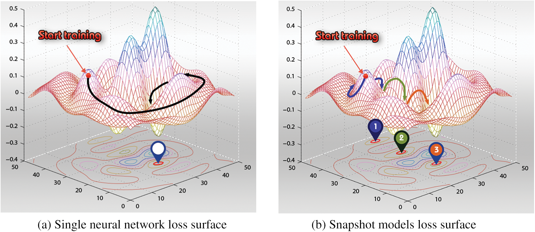
Figure 1: Exploring the loss surface, modified from [55]

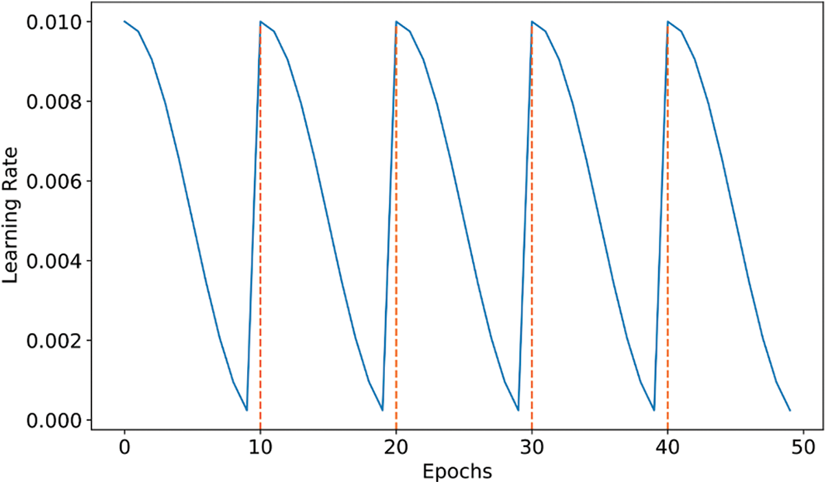
Figure 2: Cosine annealing with restart learning rate

Finally, the process is repeated N times to reach multiple convergences, each time a cycle model is obtained, and the final ensemble prediction is given by the snapshots’ model predictions mean. It was reported that such an ensemble technique results in an advantageous performance compared to the best single snapshot model [73].

α(t)=α02(cos(πmod(t−1,⌈T/N⌉)⌈T/N⌉)+1) (1)

where α0 is an initial learning rate, t is the current epoch number, T is the total training epochs, and N is the total number of cycles.

3.2 Transformer Model

The Transformer model is composed of a stack of encoder layers (Fig. 3a), a stack of decoder layers (Fig. 3b, and a linear layer followed by a fully connected layer (employing SoftMax activation function) to predict the upcoming output probabilities in a given sequence, as shown in Fig. 3. The encoder stack, as shown in Fig. 3a, consists of a stack of encoder layers, each layer embodied a multi-headed self-attention technique followed by a fully connected layer. Further, two residual connections after each of the two layers are added and connected to the normalization layers.

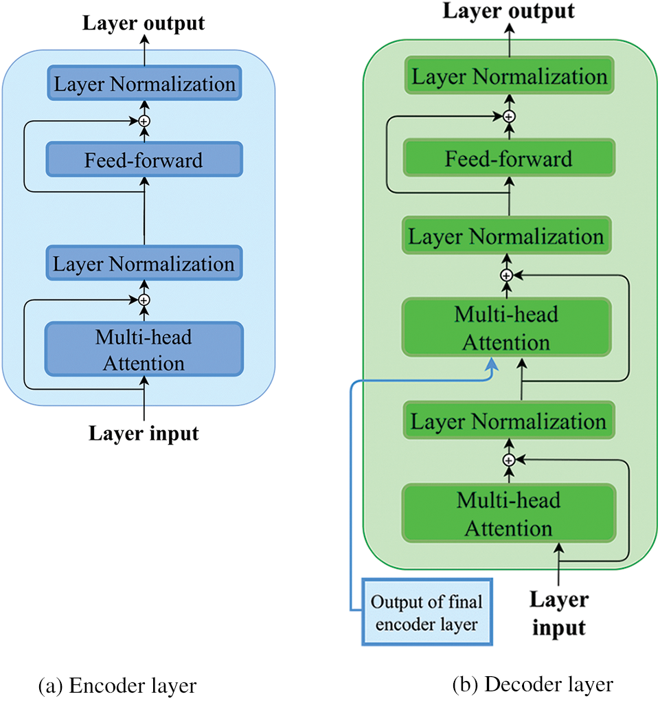
Figure 3: Encoder and decoder layers architectures

The decoder stack, shown in Fig. 3b, is somehow similar. The sole difference is that the decoder layer has two multi-headed self-attention layers along with the residual connection, which is also connected to a normalization layer followed by a fully connected feed-forward network. In short, the decoder layer has the same encoder layer architecture in addition to an extra multi-headed self-attention layer that performs multi-head attention over the output of the encoder stack. Thus, the decoder stack is fed with the encoder stack’s output alongside its layer input. Finally, in the proposed model, the decoder stack output is passed through a linear transformation followed by an output layer to yield the predicted value.

Since the Transformer model has neither recurrence nor convolution operations, thus, in order for getting advantages of the order in the input sequence, input data must be aware of the relative or absolute position of input data elements. Thus, input data is injected with some information to encode its input order. For that purpose, several methods are proposed to produce such order representation (time encoding), for instance, positional encoding [74] and Time2Vec [75].

3.3 Formulation of the Proposed Model

The overall architecture of the Transformer model is depicted in Fig. 4 which combines the encoder and decoder unites (depicted in Figs. 3a and 3b) in addition to the output layer. In this section, we aim to present the utilized architecture of the Transformer model that can fit the time series forecasting problem. Unlike the original Transformer architecture, the proposed architecture drops the fully connected layer, which employs the SoftMax activation function and is located after the decoder stack, as depicted in Fig. 4. Each rectangle (encoder/decoder layer) in Fig. 4 is represented by Encoder or Decoder sub-network which is presented in Fig. 3a or Fig. 3b, respectively.

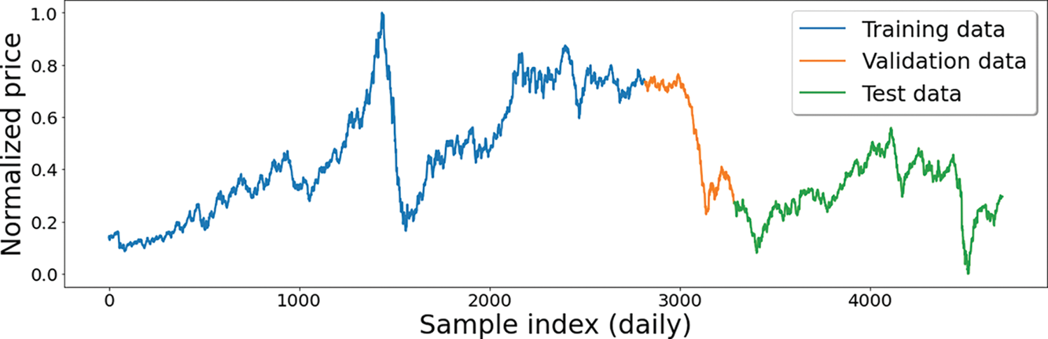
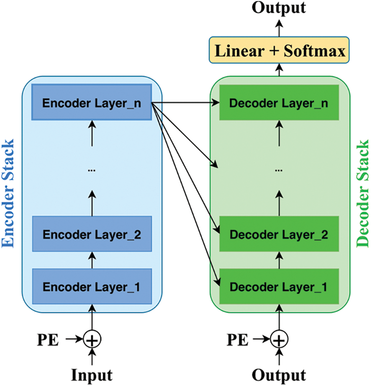
Figure 4: Transformer model architecture

Additionally, we propose investigating the possibility of using a simpler Transformer model architecture (without a decoder stack) for fast training and lower computational cost. In order to obtain the best model architecture that fits the data while maintaining good generalization performance, the model architecture is obtained by performing a grid search over a search space of parameters. Typically, model hyperparameters and their corresponding search spaces are depicted in Table 1.

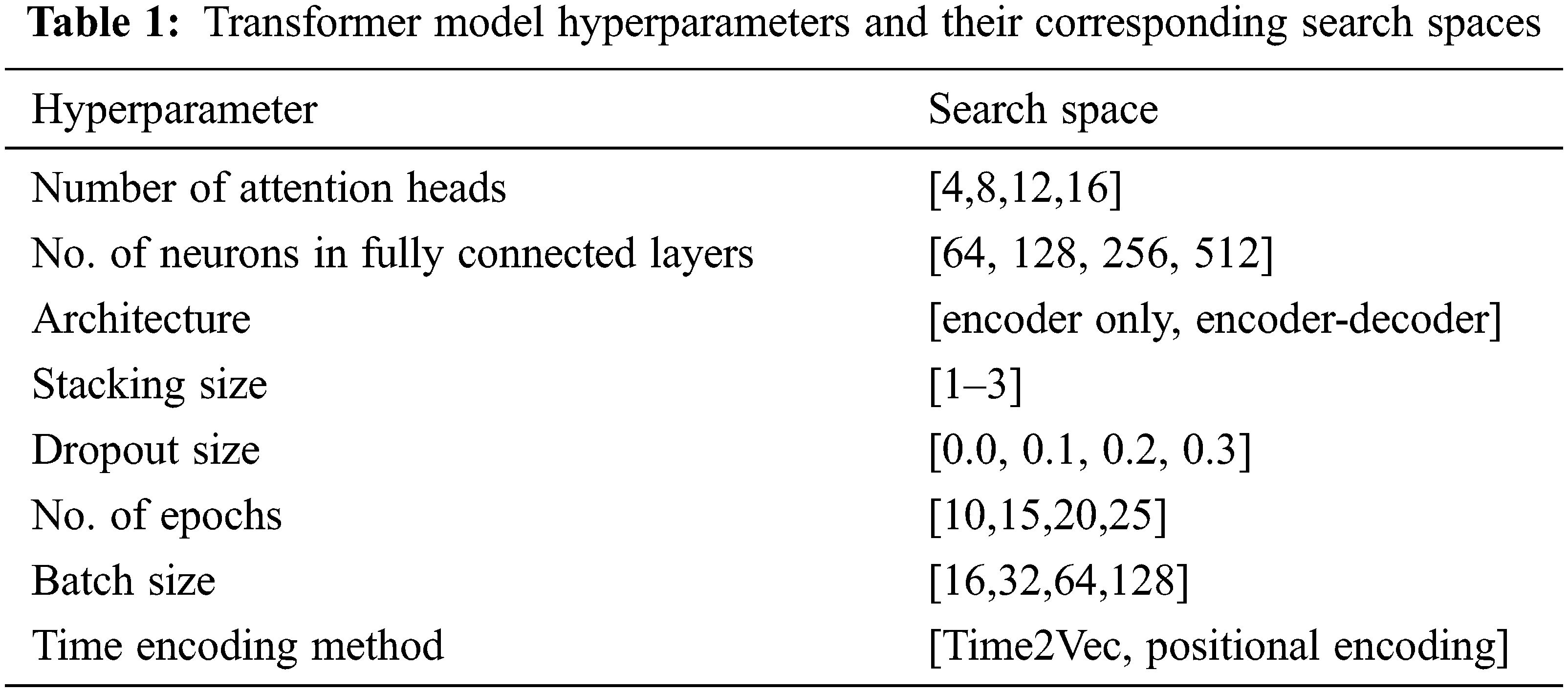
Table 1 present the model parameter search space of the of the proposed transformer model. By utilizing grid search method to find the optimal architecture, The optimal model architecture is composed of one encoder layer employing 12 attention heads, followed by a fully connected layer of 64 neurons with a Relu activation function, and finally an output layer with a linear activation function. The model is trained for 25 epochs. Each epoch of batch size equals 32 training records. For regularization purposes, we employed dropout with a rate of 0.1 in order to get more generalization performance. Finally, we employed the Adam optimizer [76] as the optimization algorithm for the proposed method. The model is trained with the objective of minimizing the mean square error objective function.

In contrast with the original snapshot method, in the proposed method, in addition to the cyclic annealing learning rate, we employ random re-initialization methods that re-initialize model parameters at the beginning of each cycle in order to surely escape the current local minima and completely explore different modes. Moreover, we initialize the model parameter at each cycle with different initialization methods (e.g., Glorot uniform [77], Glorot normal, and normal distribution) to better obtain diverse models [78].

Due to the fact that neural network models are prone to over/under-fitting problems, which are caused by the excessive/less training epochs of the neural network model [79]. Therefore, in contrast to the original snapshot method, we propose employing early stopping [80] per cycle to prevent over/under-fitting problems of the DL-based model. Consequently, each cycle stops model training (and starts the following cycle if exists) when its generalization performance starts degrading. While, for each cycle, the model that achieves better generalization performance is saved for being used in the ensemble method.

As reported in [73], the number of cycles ( N ) influences the ensemble performance. Thus, N is considered a hyperparameter that requires tuning. Consequently, the proposed snapshot ensemble is composed of N=3 snapshots of Transformer models trained for T=75 epochs, where each cycle is of a maximum of 25 epochs (depending on the early stopping method). Moreover, we employed the cyclic cosine annealing learning rate with restart at the initial learning rate α0=0.01 .

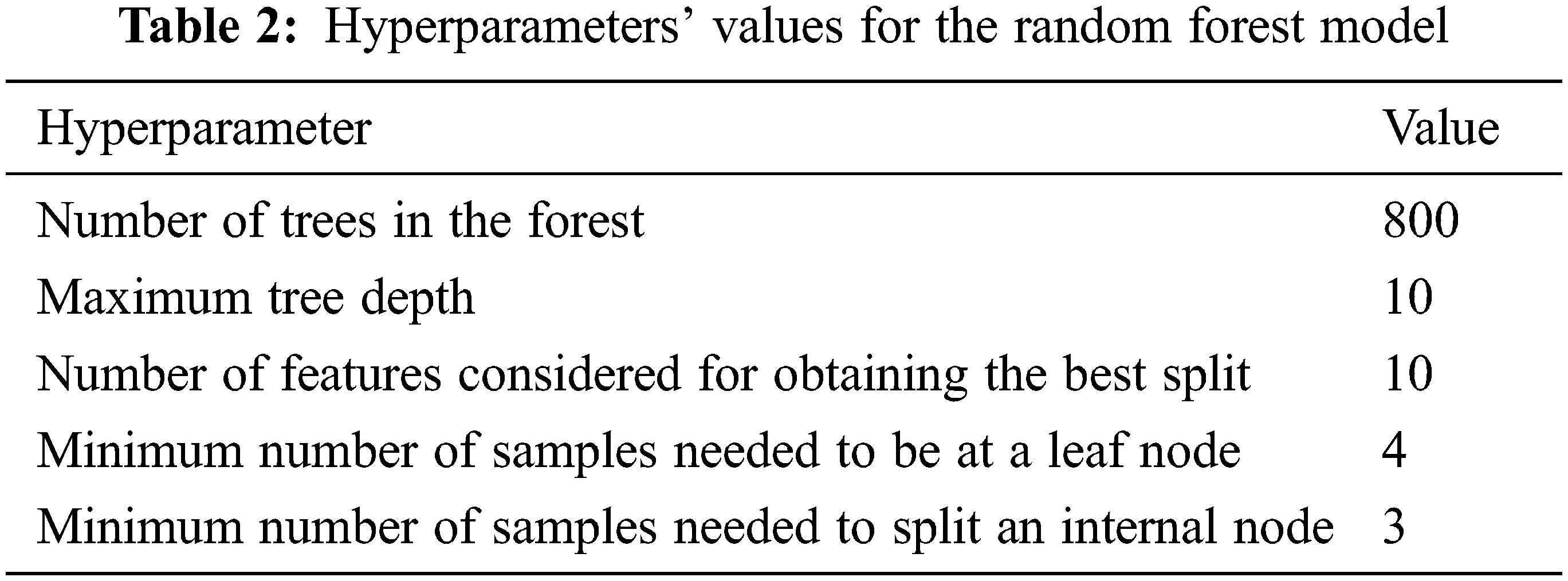
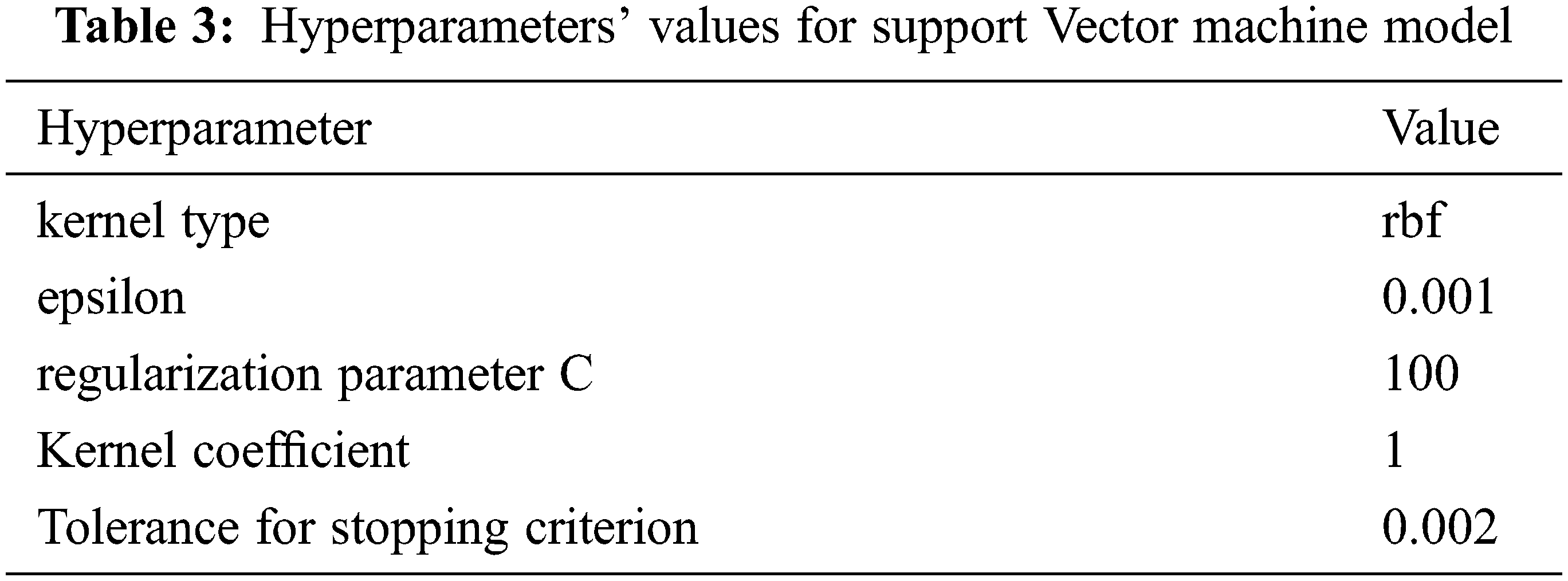
Machine learning models’ parameters are obtained using a grid search method. Therefore, hyperparameter values that resulted in obtaining the best validation scores for random forest (RF) and Support Vector Machine (SVM) models are reported in Tables 2 and 3, respectively. While other models’ parameters are set to the default value as implemented in the scikit-learn library for RF1 and SVM2.

3.4 Accuracy Metrics

For a better evaluation of the proposed forecasting models’ performance, we employ numerous widely used time series forecasting evaluation metrics [23]. Therefore, three forecasting metrics are employed, namely, mean absolute error (MAE), root mean square error (RMSE), and mean square error (MSE). The performance metrics are defined as follows:

Meanabsoluteerror(MAE)=1n.∑t=1n|yi−y^i| (2)

Rootmeansquareerror(RMSE)=1n∑t=1n(yi−y^i)2 (3)

Meansquareerror(MSE)=1n∑t=1n(yi−y^i)2 (4)

where n denotes the number of test-set data records, yi represents the actual observation values, and y^i is the model output values.

3.5 Empirical Studies

In this section, we describe the dataset used in this study and we explore the correlation between the predictors. Then, we assess the effectiveness of the suggested Snapshot ensemble of the Transformer system for predicting oil price swings. Moreover, we evaluate the predictive capacity of the proposed model against statistical, machine learning and random walk models. The comparative statistical models include ARIMA (1,1,1), ARIMA (0,1,1), ARMA (0,1), and VAR models. While baseline machine learning models are SVM and RF. All models are evaluated utilizing the same test dataset. Eventually, the fourth subsection is dedicated to analyzing the outcomes statistically.

3.6 Data Description

The data utilized in this study incorporated daily records of the OPEC crude oil prices ($/barrel) from January 2, 2003, to December 31, 2020. The data is split into training, validation, and test sets in splitting ratios of 60%, 10%, and 30%, respectively, as shown in Fig. 5.

Figure 5: The historical OPEC crude oil prices starting from January 2, 2003, to December 31, 2020

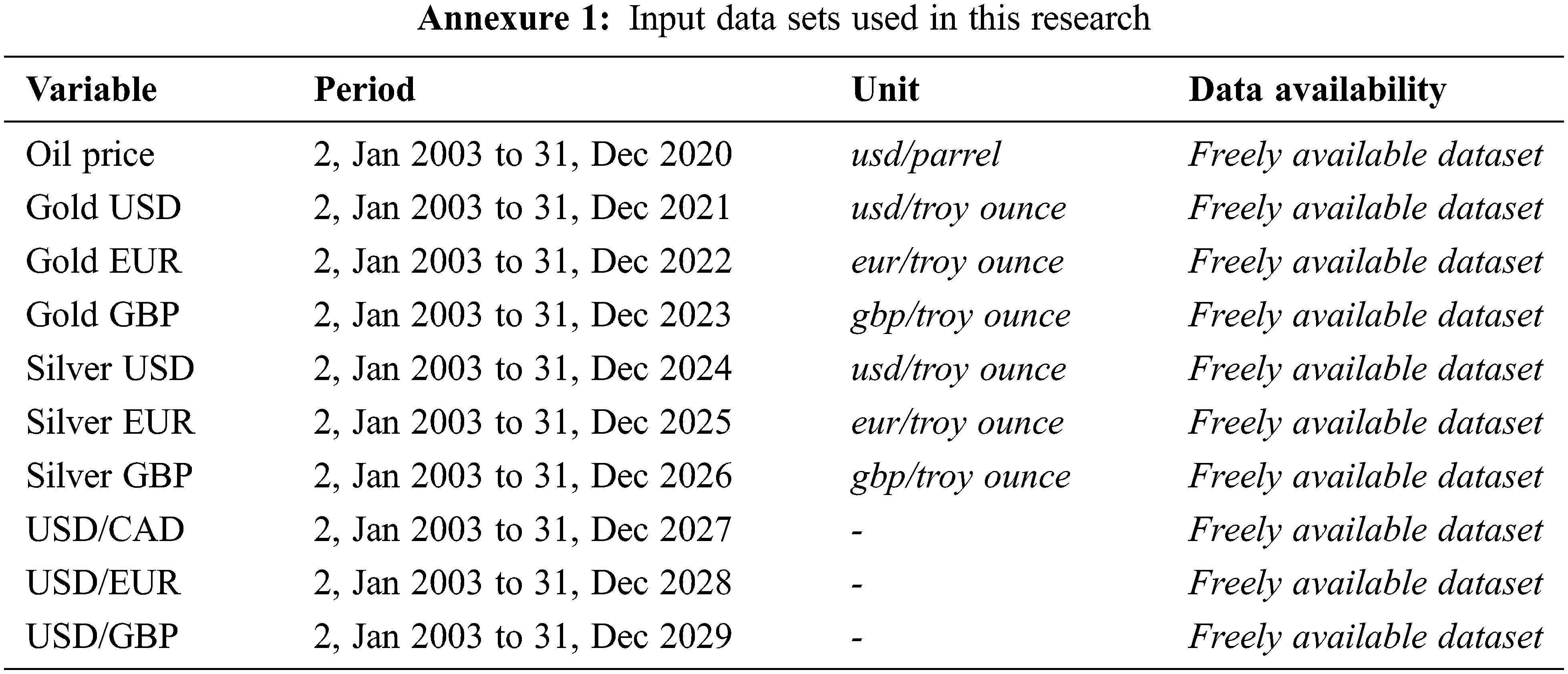
Meanwhile, performance results are reported using the test set. Typically, the validation set is beneficial for machine learning and deep learning models [81], whereas statistical models are fitted using training and validation sets. Train-validation splitting is a crucial practical tip while training machine learning and deep learning models to get better generalization performance and is used in almost all machine learning problems [82]. A crucial step in creating a consistent model is the precise choice of the variables. Thus, in this study, we specified ten predictors to enhance the forecasting models’ performance. Those predictors include silver and gold prices in three currencies, namely, USD, GBP, and EUR. In addition to the exchange rates of USD to CAD, EUR, and GBP, in addition to the past OPEC crude oil prices. The data used in this study was gathered from different sources, as illustrated in Table 4 (available in Annexure 1).

The input variables (i.e., predictors) comprise various financial indicators of diverse scales and domains. Consequently, in this study, normalizing data is beneficial in obtaining a homogeneous dataset. As a result, we normalized each variable Xi to Xi(norm) using the following equation.

Xi(norm)=Xi−XminXmax−Xmin,i=1,2,3,………,4697 (5)

where Xmin and Xmax represent the minimum and maximum values of the original data series, respectively.

3.7 Correlation Analysis

The main motivation behind correlation analysis is to investigate and explore the relation between crude oil prices (response variable) and the input predictors. Various research has substantiated that correlation is a robust method for deciding the relationship among examined variables [22,23]. To clearly explain a relationship between two variables, the correlation is primarily focused on establishing the association between two rationally connected variables and recognizing the relationship’s direction and strength. It suggests that the relationship between variables is either positive or negative in direction [83].

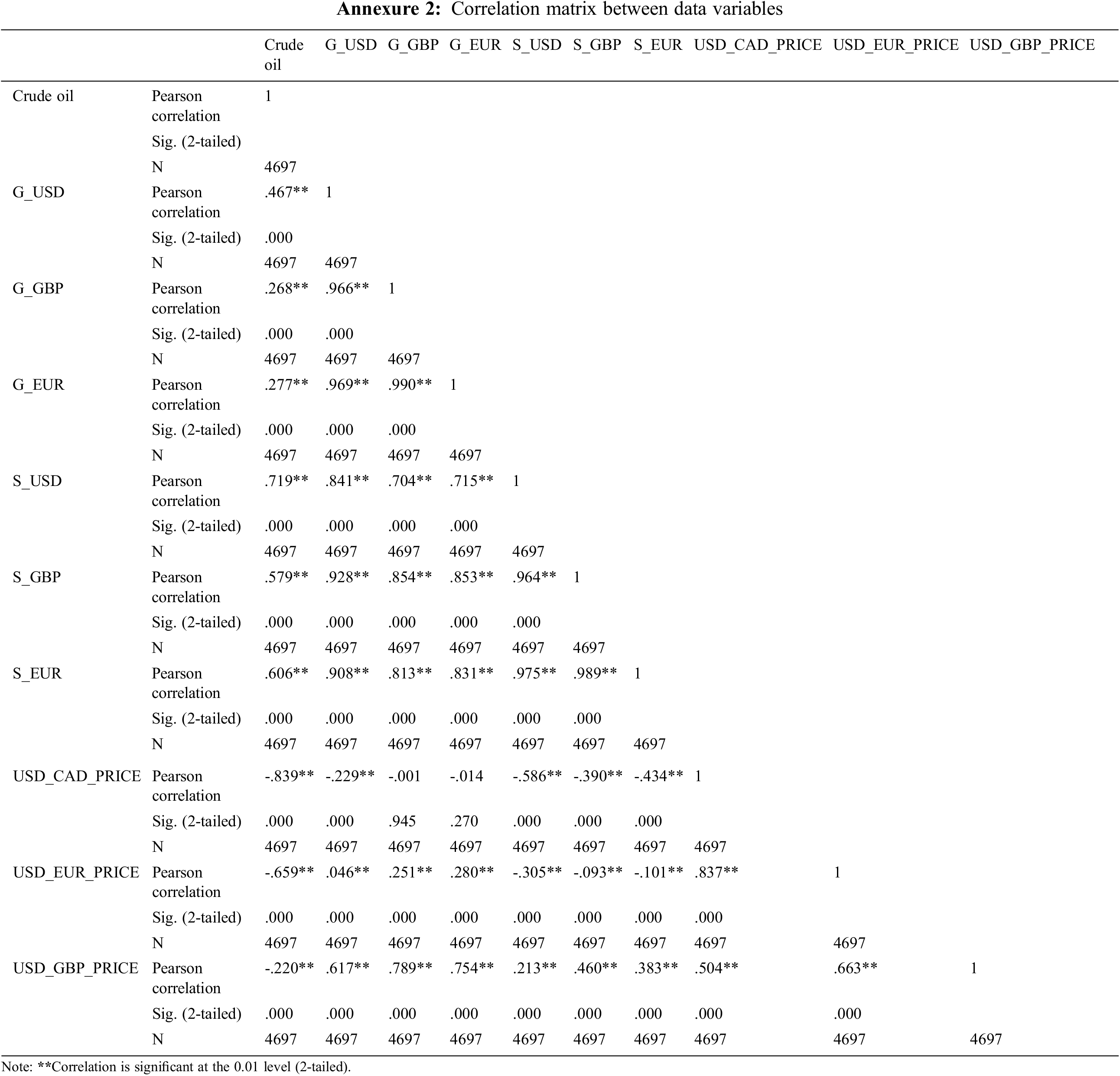
Pearson’s correlation coefficient is employed in this research to estimate the relationship between oil prices and their predictors, as illustrated by Table 5 (available in Annexure 2). Pearson’s correlation examines the existence of a correlation between two given variables, the resulting value is a number between [−1, 1]. The +1 value denotes a completely positive correlation, while the zero shows an immense statistical significance, with a p-value < 0.01.

4  Results and Discussions

In this section, we examine the efficacy of the suggested model and its comparative statistical and machine learning models (ARIMA (1,1,1), ARIMA (0,1,1), ARMA (0,1), VAR, SVM, and RF). Considerably, various studies have proved that these comparative models possess an extreme degree of precision, and these models have been used for enhancing the forecasting of different problems. Typically, the comparative models are efficient methods and are widely used in forecasting commodity prices [84–86].

4.1 Experimental Results

Table 6 presents the execution behavior of the utilized methods using 3 different performance metrics (MAE, MSE, and RMSE). The results confirm and demonstrate the high capacity and strong ability of the predictors to forecast the price volatility of crude oil. Such significant outcomes validate the importance the correlation holds between crude oil prices and all the predictors. The validation course of action that was used in this study was to assess the efficacy of the suggested model, in which the last 30% of the data were employed as a test set. The results of this assessment are depicted in Table 6. The suggested Snapshot ensemble method provides the lowest MAE, MSE, and RMSE among its competitive models used in this study. Such high performance indicates that the variation in data is strongly expressed by the fitted model. In addition, the proposed method was able to generalize and is highly probable to perform better than comparative methods when examined against other extra test periods.

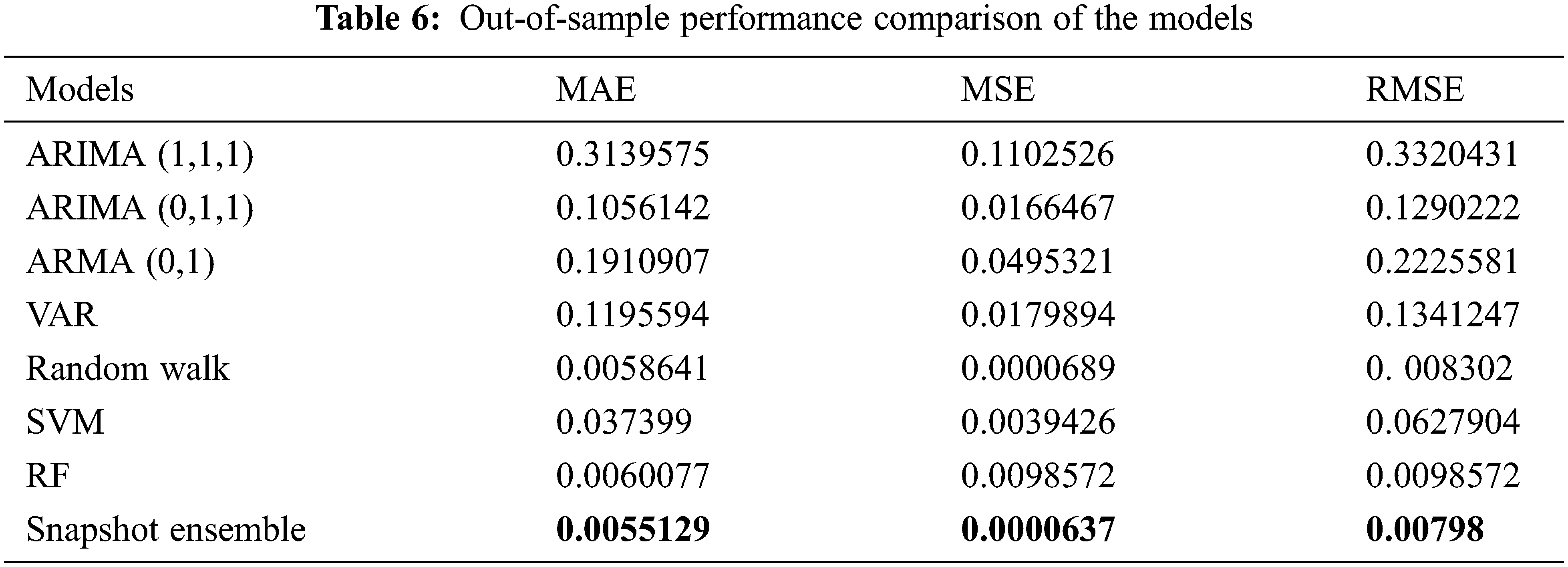
Table 7 outlines the enhancement ratio of the snapshot ensemble method in contrast to different comparative models. The suggested method clearly showed various significant contributions to raising the performance of the task at hand. Additionally, the predicted values of each model (ARIMA (1,1,1), ARIMA (0,1,1), ARMA (0,1), VAR, random walk, RF, SVM, and Snapshot ensemble models) for the test data are presented in Fig. 6.

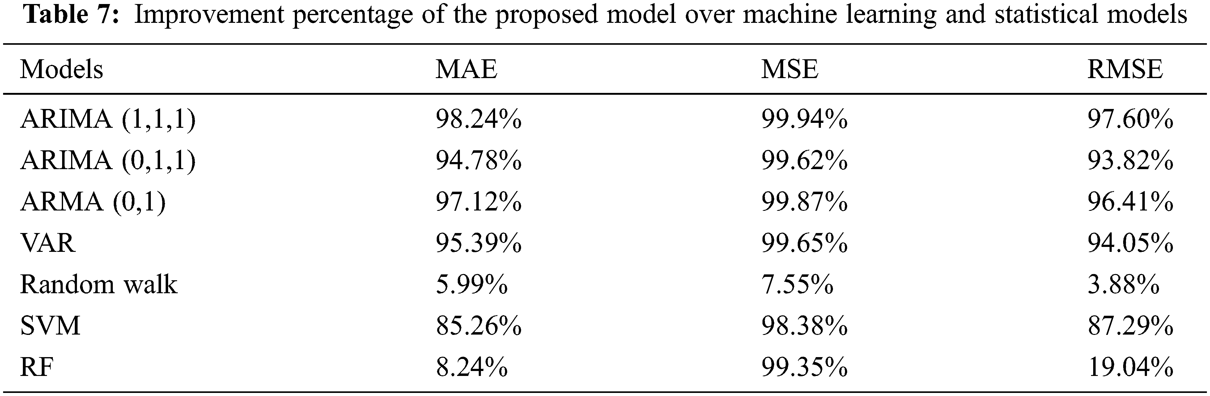
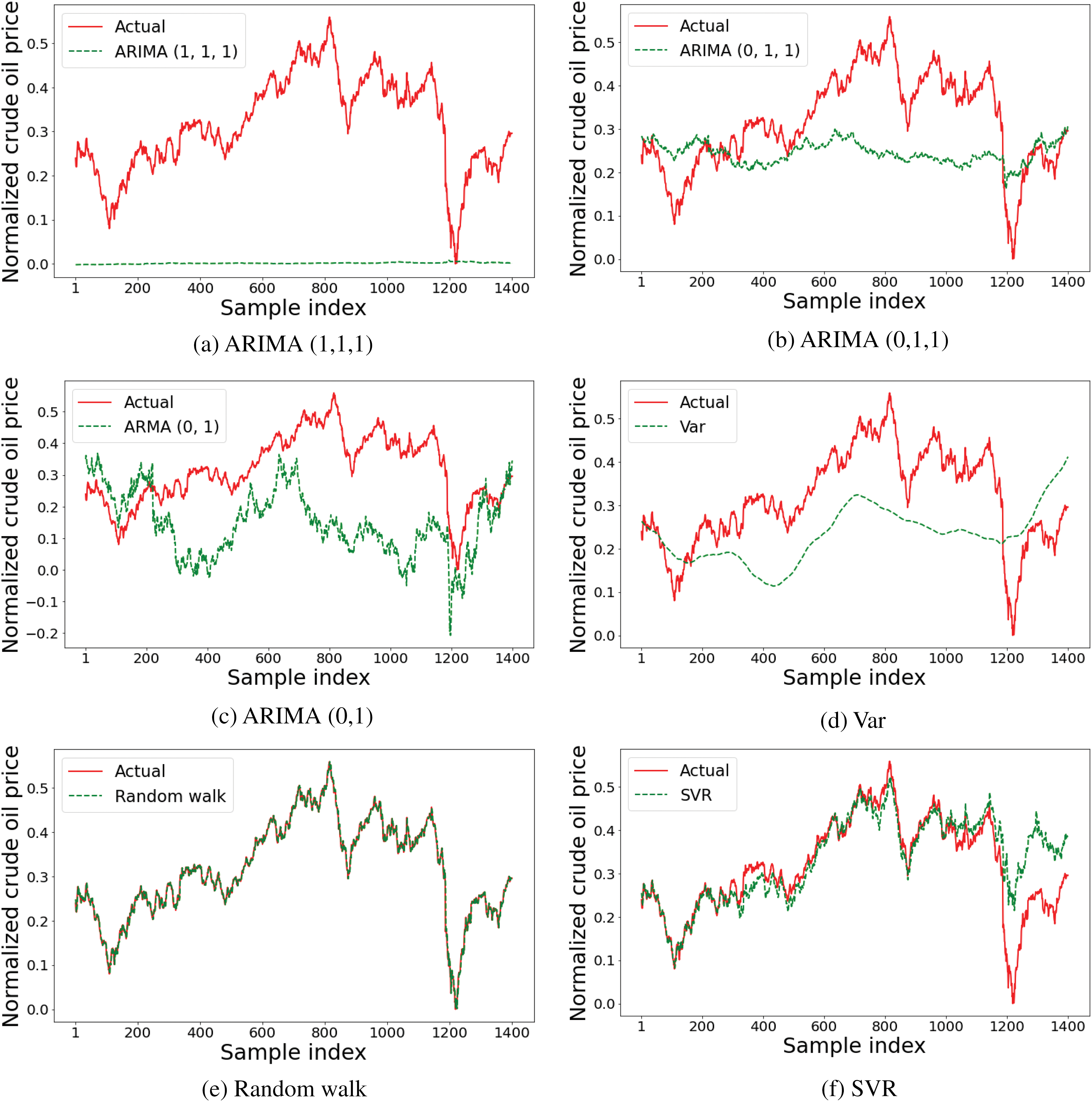
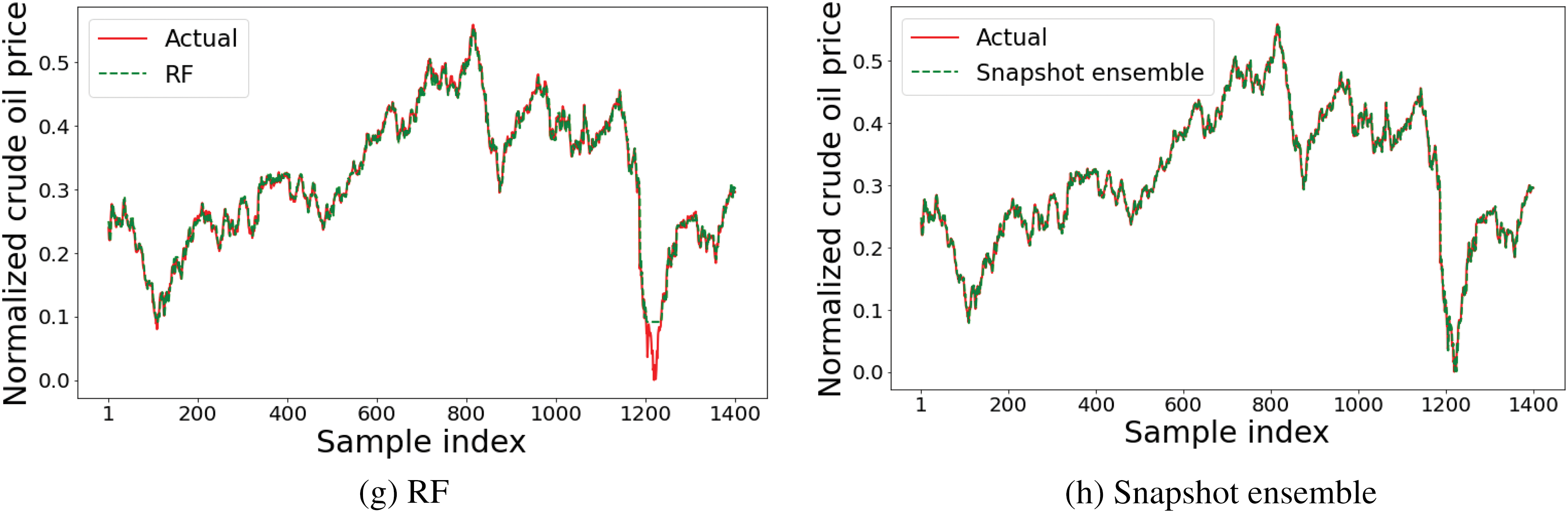
Figure 6: Performances of ARIMA (1,1,1), ARIMA (0,1,1), ARMA (0,1), VAR, Random walk, SVM, RF, and Snapshot ensemble models using the test set

Finally, it is worthwhile to point out two main reasons behind implementing a variant snapshot method than that one implemented in [73]. Firstly, applying the original snapshot resulted in very similar models’ performance, which motivated us to look for a way to obtain different variant methods. Therefore, we implemented random and different re-initialization methods of the model’s parameters at the beginning of each cycle to ensure exploring different modes in function space [78]. Theoretically, each re-initialized (i.e., cycle) model should explore different parameter spaces that other cycles’ models did not benefit from during the optimization of other cycles [73]. It is noteworthy that Huang et al. [66] reported better performance of snapshot of randomly initialized cycle’s model in the case of a high training budget.

The second reason is that implementing the original snapshot method has not yielded perfectly converged models and/or, for some cycles, it results in over-fitted models by the end of those cycles, depending on the loss surface path a model is moving on. Such csycles’ models are weak and degrade the snapshot ensemble performance. Consequently, we proposed increasing each cycle length (epochs) alongside performing early stopping per cycle to obtain the best cycle model for each cycle. Although the proposed early stopping per cycle often reduces cycle length, generally, the proposed implementation of snapshot ensemble variant imposes more training time and epochs due to each cycle is trained from scratch, in contrast to the original snapshot where cycles models (for cycles =2,…,N ) get advantages from the optimization of previous cycle relevance.

4.2 Statistical Analysis

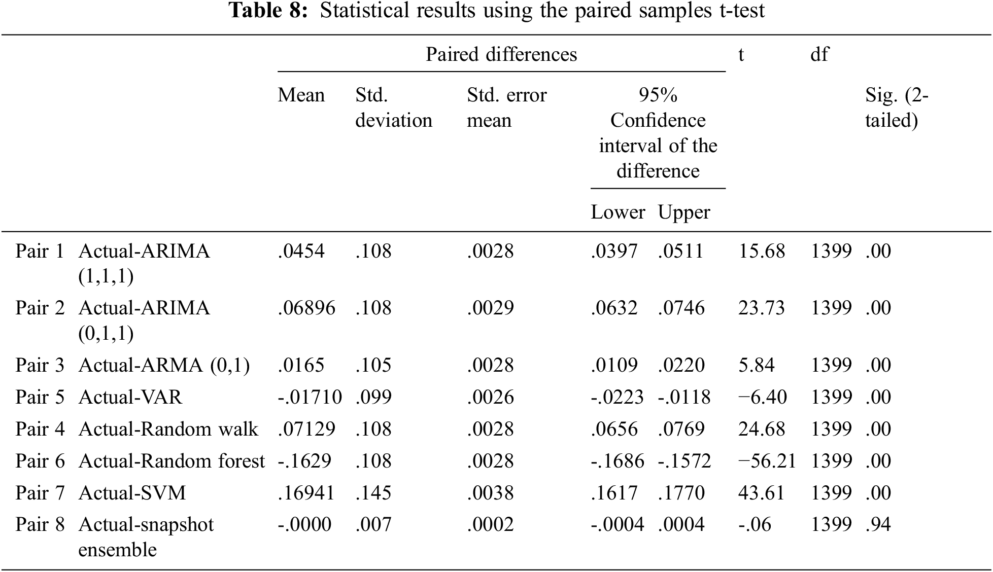
In order to highlight the outperformance of the suggested model over the conventional competitive models, we perform a significant statistical test using the predicted and actual values. Therefore, we utilized the well-known paired samples t-test [87] using the null hypothesis. A paired samples t-test is used to examine the existence of a remarkable distinction between the actual values and the forecasted values of ARIMA (1,1,1), ARIMA (0,1,1), ARMA (0,1), VAR, random walk, SVM, RF, and the proposed Snapshot Ensemble method depending on a 95% interval of confidence. The paired sample t-test is composed of two competing hypotheses (i.e., the null hypothesis and the alternative hypothesis). The two hypotheses are given by the following equations (Eq. (6)).

Ho:μ1−μ2=0,H1:μ1−μ2≠0 (6)

where μ1 is the mean value of the actual data, and μ2 represents the average of the forecasted values for the proposed methods. As presented in Table 8 the null hypothesis can be rejected at the significance level of 0.05 according to the paired samples t-test. More precisely, Table 8 depicts the paired samples t-test output for all pairs of ARIMA (1,1,1), ARIMA (0,1,1), ARMA (0,1), VAR, random walk, RF, SVM, and Snapshot Ensemble against the actual values over the test set, respectively. Consequently, the significance of the statistical t-test results demonstrates a difference among the ARIMA (1,1,1), ARIMA (0,1,1), ARMA (0,1), VAR, random walk, RF, and SVM models in opposition to the actual values; in contrast, the difference between the suggested method and the actual values shows no significance.

To sum up, according to the aforementioned points, we presented that the suggested method can be effectively implemented for predicting OPEC daily oil price variations. Moreover, we validated that this methodology is not limited to predicting the oil price but also different commodities, all metals, and ores as well.

5  Conclusion and Future Scope

Crude oil prices sustain an immense impact on the global economic dynamics. Proposing an effectively accurate method to forecast the price is substantially beneficial to pave the way for experts to make the right decisions. In this research we carefully examined the forecasting significance of a set of chosen predictors (Canadian dollar (CAD), Euro (EUR), and British Pound (GBP); and three silver prices USD, EUR, and GBP per troy ounce; three gold prices (USD, EUR, and GBP per troy ounce, and past OPEC crude oil prices) to predict future crude oil prices. Furthermore, we inspected the correlation between the response variable and predictors employing a long-term data set (from January 2, 2003, to December 31, 2020). By employing the selected predictors, we presented a deep learning ensemble method for predicting OPEC oil price fluctuations, namely, snapshot ensemble of the Transformer model. The performance of the proposed method is assessed against comparative statistical and machine learning models. The outcome prediction values proved that the snapshot ensemble of the transformer model enhanced the accuracy of forecasting compared to the ARIMA (1,1,1), ARIMA (0,1,1), ARMA (0,1), VAR, RW, SVM, and RF models by a 97.60%, 93.82%, 96.41%, 94.05%, 3.88%, 87.29%, and 19.04% improvement in RMSE, respectively. Due to the exceptional superiority of the snapshot ensemble of the transformer method over the comparative models, the proposed snapshot ensemble of the transformer model is considered to be a successful technique for predicting the prices of various commodities with a high degree of precision. In the future work, the proposed ensemble model can be validated to predict other financial market variables. Additionally, other predictors can be examined in the prediction process.

Funding Statement: The authors received no specific funding for this study.

Conflicts of Interest: The authors declare that they have no conflicts of interest to report regarding the present study.

1https://scikitlearn.org/stable/modules/generated/sklearn.ensemble.RandomForestRegressor.html

2https://scikit-learn.org/stable/modules/generated/sklearn.svm.SVR.html

Annexure

References

1. M. Mehrara, “The asymmetric relationship between oil revenues and economic activities: The case of oil-exporting countries,” Energy Policy, vol. 36, no. 3, pp. 1164–1168, 2008. [Google Scholar]
2. I. Karakurt, “Modelling and forecasting the oil consumptions of the BRICS-T countries,” Energy, vol. 220, pp. 1–11, 2021. [Google Scholar]
3. S. Śmiech, M. Papież, M. Rubaszek and M. Snarska, “The role of oil price uncertainty shocks on oil-exporting countries,” Energy Economics, vol. 93, pp. 105028, 2021. [Google Scholar]
4. L. Yu, W. Dai, L. Tang and J. Wu, “A hybrid grid-GA-based LSSVR learning paradigm for crude oil price forecasting,” Neural Computing and Applications, vol. 27, no. 8, pp. 2193–2215, 2016. [Google Scholar]
5. H. Abdollahi, “A novel hybrid model for forecasting crude oil price based on time series decomposition,” Applied Energy, vol. 267, pp. 1–12, 2020. [Google Scholar]
6. C. H. Canbaz, Y. Palabiyik, D. Putra, A. Asena, R. Ranjith et al., “A comprehensive review of smart/intelligent oilfield technologies and applications in the oil and gas industry,” in SPE Middle East Oil and Gas Show and Conf., Manama, Bahrain, 2019. [Google Scholar]
7. A. Sircar, K. Yadav, K. Rayavarapu, N. Bist and H. Oza, “Application of machine learning and artificial intelligence in oil and gas industry,” Petroleum Research, vol. 6, pp. 379–391, 2021. [Google Scholar]
8. B. Wu, L. Wang, S. -X. Lv and Y. -R. Zeng, “Effective crude oil price forecasting using new text-based and big-data-driven model,” Measurement, vol. 168, pp. 108468, 2021. [Google Scholar]
9. Y. Huang and Y. Deng, “A new crude oil price forecasting model based on variational mode decomposition,” Knowledge-Based Systems, vol. 213, pp. 106669, 2021. [Google Scholar]
10. Y. Lyu, S. Tuo, Y. Wei and M. Yang, “Time-varying effects of global economic policy uncertainty shocks on crude oil price volatility: New evidence,” Resources Policy, vol. 70, pp. 101943, 2021. [Google Scholar]
11. S. H. Hosseini, H. Shakouri and A. Kazemi, “Oil price future regarding unconventional oil production and its near-term deployment: A system dynamics approach,” Energy, vol. 222, pp. 1–12, 2021. [Google Scholar]
12. M. Abd Elaziz, A. A. Ewees and Z. Alameer, “Improving adaptive neuro-fuzzy inference system based on a modified salp swarm algorithm using genetic algorithm to forecast crude oil price,” Natural Resources Research, vol. 29, no. 4, pp. 2671–2686, 2020. [Google Scholar]
13. E. Panopoulou and T. Pantelidis, “Speculative behaviour and oil price predictability,” Economic Modelling, vol. 47, pp. 128–136, 2015. [Google Scholar]
14. Y. Wei, Y. Wang and D. Huang, “Forecasting crude oil market volatility: Further evidence using GARCH-class models,” Energy Economics, vol. 32, no. 6, pp. 1477–1484, 2010. [Google Scholar]
15. C. Zhao and B. Wang, “Forecasting crude oil price with an autoregressive integrated moving average (ARIMA) model,” in Fuzzy Information & Engineering and Operations Research & Management, Berlin, Heidelberg, Germany: Springer, pp. 275–286, 2014. [Google Scholar]
16. A. Lanza, M. Manera and M. Giovannini, “Modeling and forecasting cointegrated relationships among heavy oil and product prices,” Energy Economics, vol. 27, no. 6, pp. 831–848, 2005. [Google Scholar]
17. L. Yu, Y. Zhao and L. Tang, “A compressed sensing based AI learning paradigm for crude oil price forecasting,” Energy Economics, vol. 46, pp. 236–245, 2014. [Google Scholar]
18. A. Al-Ghandoor, M. Samhouri, I. Al-Hinti, J. Jaber and M. Al-Rawashdeh, “Projection of future transport energy demand of Jordan using adaptive neuro-fuzzy technique,” Energy, vol. 38, no. 1, pp. 128–135, 2012. [Google Scholar]
19. Y. Chen, K. He and G. K. Tso, “Forecasting crude oil prices: A deep learning based model,” Procedia Computer Science, vol. 122, pp. 300–307, 2017. [Google Scholar]
20. A. Safari and M. Davallou, “Oil price forecasting using a hybrid model,” Energy, vol. 148, pp. 49–58, 2018. [Google Scholar]
21. Z. Alameer, M. Abd Elaziz, A. A. Ewees, H. Ye and Z. Jianhua, “Forecasting gold price fluctuations using improved multilayer perceptron neural network and whale optimization algorithm,” Resources Policy, vol. 61, pp. 250–260, 2019. [Google Scholar]
22. Z. Alameer, A. Fathalla, K. Li, H. Ye and Z. Jianhua, “Multistep-ahead forecasting of coal prices using a hybrid deep learning model,” Resources Policy, vol. 65, pp. 101588, 2020. [Google Scholar]
23. A. A. Ewees, M. Abd Elaziz, Z. Alameer, H. Ye and Z. Jianhua, “Improving multilayer perceptron neural network using chaotic grasshopper optimization algorithm to forecast iron ore price volatility,” Resources Policy, vol. 65, pp. 101555, 2020. [Google Scholar]
24. J. Wang, X. Niu, Z. Liu and L. Zhang, “Analysis of the influence of international benchmark oil price on China’s real exchange rate forecasting,” Engineering Applications of Artificial Intelligence, vol. 94, pp. 103783, 2020. [Google Scholar]
25. Y. -C. Chen, K. S. Rogoff and B. Rossi, “Can exchange rates forecast commodity prices?” The Quarterly Journal of Economics, vol. 125, no. 3, pp. 1145–1194, 2010. [Google Scholar]
26. B. Atems, D. Kapper and E. Lam, “Do exchange rates respond asymmetrically to shocks in the crude oil market?” Energy Economics, vol. 49, pp. 227–238, 2015. [Google Scholar]
27. J. Beckmann, T. Berger and R. Czudaj, “Oil price and FX-rates dependency,” Quantitative Finance, vol. 16, no. 3, pp. 477–488, 2016. [Google Scholar]
28. J. Beckmann and R. Czudaj, “Is there a homogeneous causality pattern between oil prices and currencies of oil importers and exporters?” Energy Economics, vol. 40, pp. 665–678, 2013. [Google Scholar]
29. R. A. Lizardo and A. V. Mollick, “Oil price fluctuations and US dollar exchange rates,” Energy Economics, vol. 32, no. 2, pp. 399–408, 2010. [Google Scholar]
30. J. C. Reboredo, “Modelling oil price and exchange rate co-movements,” Journal of Policy Modeling, vol. 34, no. 3, pp. 419–440, 2012. [Google Scholar]
31. J. C. Reboredo, M. A. Rivera-Castro and G. F. Zebende, “Oil and US dollar exchange rate dependence: A detrended cross-correlation approach,” Energy Economics, vol. 42, pp. 132–139, 2014. [Google Scholar]
32. Y. He, S. Wang and K. K. Lai, “Global economic activity and crude oil prices: A cointegration analysis,” Energy Economics, vol. 32, no. 4, pp. 868–876, 2010. [Google Scholar]
33. S. Lardic and V. Mignon, “Oil prices and economic activity: An asymmetric cointegration approach,” Energy Economics, vol. 30, no. 3, pp. 847–855, 2008. [Google Scholar]
34. N. B. Behmiri and M. Manera, “The role of outliers and oil price shocks on volatility of metal prices,” Resources Policy, vol. 46, pp. 139–150, 2015. [Google Scholar]
35. R. Chen and J. Xu, “Forecasting volatility and correlation between oil and gold prices using a novel multivariate GAS model,” Energy Economics, vol. 78, pp. 379–391, 2019. [Google Scholar]
36. S. Kumar, “On the nonlinear relation between crude oil and gold,” Resources Policy, vol. 51, pp. 219–224, 2017. [Google Scholar]
37. P. Li and Z. Dong, “Time-varying network analysis of fluctuations between crude oil and Chinese and US gold prices in different periods,” Resources Policy, vol. 68, pp. 101749, 2020. [Google Scholar]
38. S. Husain, A. K. Tiwari, K. Sohag and M. Shahbaz, “Connectedness among crude oil prices, stock index and metal prices: An application of network approach in the USA,” Resources Policy, vol. 62, pp. 57–65, 2019. [Google Scholar]
39. A. K. Tiwari, B. R. Mishra and S. A. Solarin, “Analysing the spillovers between crude oil prices, stock prices and metal prices: The importance of frequency domain in USA,” Energy, vol. 220, pp. 1–18, 2021. [Google Scholar]
40. D. Ç. Yıldırım, E. I. Cevik and Ö. Esen, “Time-varying volatility spillovers between oil prices and precious metal prices,” Resources Policy, vol. 68, pp. 101783, 2020. [Google Scholar]
41. T. Kriechbaumer, A. Angus, D. Parsons and M. R. Casado, “An improved wavelet–ARIMA approach for forecasting metal prices,” Resources Policy, vol. 39, pp. 32–41, 2014. [Google Scholar]
42. N. Dilshad and J. Song, “Dual-stream siamese network for vehicle re-identification via dilated convolutional layers,” in IEEE Int. Conf. on Smart Internet of Things (SmartIoT), Jeju Island, SK, pp. 350–352, 2021. [Google Scholar]
43. S. Ullah Khan, I. Ul Haq, S. Rho, S. Wook Baik and M. Young Lee, “Cover the violence: A novel deep-learning-based approach towards violence-detection in movies,” Applied Sciences, vol. 9, no. 22, pp. 4963, 2019. [Google Scholar]
44. A. Ali, A. Fathalla, A. Salah, M. Bekhit and E. Eldesouky, “Marine data prediction: An evaluation of machine learning, deep learning, and statistical predictive models,” Computational Intelligence and Neuroscience, vol. 2021, pp. 5777, 2021. [Google Scholar]
45. E. Eldesouky, M. Bekhit, A. Fathalla, A. Salah and A. Ali, “A robust UWSN handover prediction system using ensemble learning,” Sensors, vol. 21, no. 17, pp. 5777, 2021. [Google Scholar]
46. D. Povey, H. Hadian, P. Ghahremani, K. Li and S. Khudanpur, “A time-restricted self-attention layer for ASR,” in 2018 IEEE Int. Conf. on Acoustics, Speech and Signal Processing (ICASSP), Calgary, AB, Canada, pp. 5874–5878, 2018. [Google Scholar]
47. N. Parmar, A. Vaswani, J. Uszkoreit, L. Kaiser, N. Shazeer et al., “Image transformer,” in Int. Conf. on Machine Learning, Stockholmsmässan, Stockholm, Sweden, pp. 4055–4064, 2018. [Google Scholar]
48. S. Li, X. Jin, Y. Xuan, X. Zhou, W. Chen et al., “Enhancing the locality and breaking the memory bottleneck of transformer on time series forecasting,” Advances in Neural Information Processing Systems (NeurIPS 2019), Vancouver, Canada, vol. 32, pp. 5243–5253, 2019. [Google Scholar]
49. Y. Li, C. Chen, M. Duan, Z. Zeng and K. Li, “Attention-aware encoder–decoder neural networks for heterogeneous graphs of things,” IEEE Transactions on Industrial Informatics, vol. 17, no. 4, pp. 2890–2898, 2020. [Google Scholar]
50. Z. Zhou and X. Dong, “Analysis about the seasonality of China’s crude oil import based on X-12-ARIMA,” Energy, vol. 42, no. 1, pp. 281–288, 2012. [Google Scholar]
51. P. Agnolucci, “Volatility in crude oil futures: A comparison of the predictive ability of GARCH and implied volatility models,” Energy Economics, vol. 31, no. 2, pp. 316–321, 2009. [Google Scholar]
52. A. Hou and S. Suardi, “A nonparametric GARCH model of crude oil price return volatility,” Energy Economics, vol. 34, no. 2, pp. 618–626, 2012. [Google Scholar]
53. N. Gupta and S. Nigam, “Crude oil price prediction using artificial neural network,” Procedia Computer Science, vol. 170, pp. 642–647, 2020. [Google Scholar]
54. S. Gao and Y. Lei, “A new approach for crude oil price prediction based on stream learning,” Geoscience Frontiers, vol. 8, no. 1, pp. 183–187, 2017. [Google Scholar]
55. J. Baruník and B. Malinska, “Forecasting the term structure of crude oil futures prices with neural networks,” Applied Energy, vol. 164, pp. 366–379, 2016. [Google Scholar]
56. T. Mingming and Z. Jinliang, “A multiple adaptive wavelet recurrent neural network model to analyze crude oil prices,” Journal of Economics and Business, vol. 64, no. 4, pp. 275–286, 2012. [Google Scholar]
57. L. Yu, X. Zhang and S. Wang, “Assessing potentiality of support vector machine method in crude oil price forecasting,” EURASIA Journal of Mathematics, Science and Technology Education, vol. 13, no. 12, pp. 7893–7904, 2017. [Google Scholar]
58. S. Ramyar and F. Kianfar, “Forecasting crude oil prices: A comparison between artificial neural networks and vector autoregressive models,” Computational Economics, vol. 53, no. 2, pp. 743–761, 2019. [Google Scholar]
59. W. Xie, L. Yu, S. Xu and S. Wang, “A new method for crude oil price forecasting based on support vector machines,” in Int. Conf. on Computational Science, Reading, UK, pp. 444–451, 2006. [Google Scholar]
60. A. A. Godarzi, R. M. Amiri, A. Talaei and T. Jamasb, “Predicting oil price movements: A dynamic artificial neural network approach,” Energy Policy, vol. 68, pp. 371–382, 2014. [Google Scholar]
61. H. Abdollahi, “An adaptive neuro-based fuzzy inference system (ANFIS) for the prediction of option price: The case of the Australian option market,” International Journal of Applied Metaheuristic Computing (IJAMC), vol. 11, no. 2, pp. 99–117, 2020. [Google Scholar]
62. H. Abdollahi and S. B. Ebrahimi, “A new hybrid model for forecasting Brent crude oil price,” Energy, vol. 200, pp. 1–13, 2020. [Google Scholar]
63. Y. -X. Wu, Q. -B. Wu and J. -Q. Zhu, “Improved EEMD-based crude oil price forecasting using LSTM networks,” Physica A: Statistical Mechanics and its Applications, vol. 516, pp. 114–124, 2019. [Google Scholar]
64. J. Zhu, J. Liu, P. Wu, H. Chen and L. Zhou, “A novel decomposition-ensemble approach to crude oil price forecasting with evolution clustering and combined model,” International Journal of Machine Learning and Cybernetics, vol. 10, no. 12, pp. 3349–3362, 2019. [Google Scholar]
65. J. Chai, L. -M. Xing, X. -Y. Zhou, Z. G. Zhang and J. -X. Li, “Forecasting the WTI crude oil price by a hybrid-refined method,” Energy Economics, vol. 71, pp. 114–127, 2018. [Google Scholar]
66. G. Huang, Y. Li, G. Pleiss, Z. Liu, J. E. Hopcroft et al., “Snapshot ensembles: Train 1, get m for free,” arXiv preprint arXiv:1704.00109, 2017. [Google Scholar]
67. H. Jiang, W. Hu, L. Xiao and Y. Dong, “A decomposition ensemble based deep learning approach for crude oil price forecasting,” Resources Policy, vol. 78, pp. 102855. 2022. [Google Scholar]
68. S. Ghimire, R. C. Deo, H. Wang, M. S. Al-Musaylh, D. Casillas-Pérez et al., “Stacked LSTM sequence-to-sequence autoencoder with feature selection for daily solar radiation prediction: A review and new modeling results,” Energies, vol. 15, no. 3, pp. 1061, 2022. [Google Scholar]
69. K. Alkhatib, H. Khazaleh, H. A. Alkhazaleh, A. R. Alsoud et al., “A new stock price forecasting method using active deep learning approach,” Journal of Open Innovation: Technology, Market, and Complexity, vol. 8, no. 2, pp. 96, 2022. [Google Scholar]
70. Z. Wang, Z. Wu, M. Zou, X. Wen et al., “A voting-based ensemble deep learning method focused on multi-step prediction of food safety risk levels: Applications in hazard analysis of heavy metals in grain processing products,” Foods, vol. 11, no. 6, pp. 823, 2022. [Google Scholar]
71. N. Sehgal and K. K. Pandey, “Artificial intelligence methods for oil price forecasting: A review and evaluation,” Energy Systems, vol. 6, no. 4, pp. 479–506, 2015. [Google Scholar]
72. J. L. Zhang, Y. J. Zhang and L. Zhang, “A novel hybrid method for crude oil price forecasting,” Energy Economics, vol. 49, pp. 649–659, 2015. [Google Scholar]
73. A. Vaswani, N. Shazeer, N. Parmar, J. Uszkoreit, L. Jones et al., “Attention is all you need,” in Advances in Neural Information Processing Systems (NIPS 2017), Long Beach, CA, USA: Neural Information Processing Systems Foundation, Inc. (NeurIPSpp. 5998–6008, 2017. [Google Scholar]
74. S. M. Kazemi, R. Goel, S. Eghbali, J. Ramanan, J. Sahota et al., “Time2vec: Learning a vector representation of time,” arXiv preprint arXiv:1907.05321, 2019. [Google Scholar]
75. D. P. Kingma and J. Ba, “Adam: A method for stochastic optimization,” arXiv, preprint arXiv:1412.6980, 2014. [Google Scholar]
76. X. Glorot and Y. Bengio, “Understanding the difficulty of training deep feedforward neural networks,” in Proc. of the Thirteenth Int. Conf. on Artificial Intelligence and Statistics, Sardinia, Italy, pp. 249–256, 2010. [Google Scholar]
77. S. Fort, H. Hu and B. Lakshminarayanan, “Deep ensembles: A loss landscape perspective,” arXiv preprint arXiv:1912.02757, 2019. [Google Scholar]
78. S. Geman, E. Bienenstock and R. Doursat, “Neural networks and the bias/variance dilemma,” Neural Computation, vol. 4, no. 1, pp. 1–58, 1992. [Google Scholar]
79. Y. Yao, L. Rosasco and A. Caponnetto, “On early stopping in gradient descent learning,” Constructive Approximation, vol. 26, no. 2, pp. 289–315, 2007. [Google Scholar]
80. A. Fathalla, A. Salah, K. Li, K. Li and P. Francesco, “Deep end-to-end learning for price prediction of second-hand items,” Knowledge and Information Systems, vol. 62, no. 12, pp. 4541–4568, 2020. [Google Scholar]
81. Y. Xu and R. Goodacre, “On splitting training and validation set: A comparative study of cross-validation, bootstrap and systematic sampling for estimating the generalization performance of supervised learning,” Journal of Analysis and Testing, vol. 2, no. 3, pp. 249–262, 2018. [Google Scholar]
82. K. Molugaram and G. S. Rao, “Chapter 6-correlation and regression,” Statistical Techniques for Transportation Engineering, pp. 293–329, 2017. [Google Scholar]
83. Z. -Y. Chen, “A hybrid algorithm by combining swarm intelligence methods and neural network for gold price prediction,” in Multidisciplinary Social Networks Research (MISNC 2014), Kaohsiung, Taiwan: Springer, pp. 404–416, 2014. [Google Scholar]
84. X. Fan, L. Wang and S. Li, “Predicting chaotic coal prices using a multi-layer perceptron network model,” Resources Policy, vol. 50, pp. 86–92, 2016. [Google Scholar]
85. H. F. Zou, G. P. Xia, F. T. Yang and H. Y. Wang, “An investigation and comparison of artificial neural network and time series models for Chinese food grain price forecasting,” Neurocomputing, vol. 70, no. 16–18, pp. 2913–2923, 2007. [Google Scholar]
86. M. Fritz and P. Berger, “Chapter 3–Comparing two designs (or anything else!) using paired sample T-tests,” in Improving the User Experience Through Practical Data Analytics, Boston, USA: Morgan Kaufmann, pp. 71–89, 2015. [Google Scholar]
87. N. Atluri and S. Shen, “Global weak forms, weighted residuals, finite elements, boundary elements & local weak forms,” in The Meshless Local Petrov-Galerkin (MLPG) Method, 1st ed., vol. 1. Henderson, NV, USA: Tech Science Press, pp. 15–64, 2004. [Google Scholar]
Annexure
Cite This Article
Copyright © 2023 The Author(s). Published by Tech Science Press.
This work is licensed under a Creative Commons Attribution 4.0 International License , which permits unrestricted use, distribution, and reproduction in any medium, provided the original work is properly cited.
Downloads
Citation Tools