Price Prediction of Seasonal Items Using Time Series Analysis

1  Introduction

Trading stocks and electronic commerce (e-commerce) relied heavily on intuition [1]. As both became very popular nowadays, individual’s desired strategies and instruments to correctly forecast products or share values, lowering their risk and increasing profits. Given the prevalence of e-commerce websites, it is critical to research price prediction. The primary difficulty in forecasting the product price is a chaotic system.

For instance, crude oil may be considered the engine that powers a large number of economic activities worldwide. Commercial operations inside states and international trade are heavily reliant on oil and other natural resources [2,3]. Thus, the crude oil price has a discernible effect on the global economy’s stability, and no sector of the global economy is immune to the effects of crude oil price variations. The significance of crude oil has attracted oil industry practitioners, academics, and governments’ curiosity. This is a challenging endeavor since the factors affecting the price of crude oil are impossible to anticipate or manage. Oil prices fluctuate, especially on seasonal occasions, in response to market factors, namely demand and supply pressures. However, oil prices are not immune to global events since crises that often erupt in nations worldwide (particularly volatile oil-producing nations) can enhance crude oil prices.

Numerous variables and complications might impact the selection directly or indirectly, such as the optimal time to purchase or sell items, commodities, or seasonal presents. Stockholders must determine when to sell in the financial market, and customers must obtain things at reasonable rates. As a result, the issue of price prediction has developed. In addition, several approaches, including technical, statistical, fundamental analysis, and machine learning, have been developed to anticipate the prices of products. These models can forecast the values of a variety of financial assets, including cryptocurrencies, oil, stocks, gold, and used products.

Financial market forecasting is a difficult endeavor because financial time series are noisy, non-stationary, and irregular as a result of too many diverse factors affecting the magnitude and frequency of stock rises and falls at the same time [4]. Although there are numerous statistical and computational approaches for predicting these series, they produce imprecise results because most variables in financial markets follow a nonlinear pattern.

ML and DL have become innovative approaches for financial data analysis in recent years. DL’s advantages, such as automatic feature learning, multilayer feature learning, high precision in results, high generalization power, and the ability to identify new data, make it an appropriate approach for predicting financial markets [5].

Recent improvements in ML and DL structures have exhibited state-of-the-art performance in a variety of applications [6,7], such as text processing, pictures, speech, and audio on a variety of natural language processing (NLP) and computer vision applications, which include language modeling [8], speech recognition [9,10], computer vision [11], sentence classification [12] and machine translation [13]. Typically, ML and DL have become innovative approaches for financial data analysis in recent years. DL’s advantages, such as automatic feature learning, multilayer feature learning, high precision in results, high generalization power, and the ability to identify new data, make it an appropriate approach for predicting financial markets [1,2,5,14].

The motivation of this paper is the limited works of predicting the prices of seasonal items. In the literature, there is a single instance in which seasonal product price prediction was presented as a regression problem. Consequently, this paper addresses the formulation of the challenge related to predicting seasonal item prices as a time series problem. In other words, it includes the date characteristics in the problem. In addition, this work evaluates the performance of ML and DL models to determine the disparity between their prediction accuracy rates. The following are the primary contributions of this work:

•   To our knowledge, this is the first work to propose framing the task of price prediction of seasonal items (i.e., gifts) as a time series prediction task.

•   To our knowledge, this is the first time to utilize the GRU deep neural network (DNN) architecture to handle the problem of seasonal items’ prices prediction.

•   We proposed a new stacked GRU-DNN architecture to predict the seasonal items’ prices.

•   The proposed predictive system was evaluated on a real-life dataset to compare the performance of ML and DL methods.

The remainder of the paper is structured as follows: Section 2 describes the most recent techniques related to work. Then, in Section 3, the suggested system for seasonal item price prediction is described. Section 4 details the experimental outcomes of the proposed system’s evaluation. The work is concluded in Section 5.

2  Related Work

In this section, the literature on price prediction is discussed based to expose the different ML and DL methods which are proposed in this context. The discussed methods predicted the prices of different several goods. Of note, the discussion outlines the utilized accuracy metrics which are used to evaluate the proposed methods.

2.1 Deep Learning Methods

DL techniques, in particular recurrent neural networks (RNNs), have been shown to be effective in a variety of applications, one of which is time series forecasting, where they have been utilized [2,6,15]. Diverse applications, including time series forecasting, have demonstrated the effectiveness of DL approaches. RNN is a dependable model that can discover an infinite number of complex relationships from an arbitrarily large data source. It has been utilized effectively to resolve a number of problems, and it continues to discover new applications in this field. It has also been used to effectively handle a vast array of other issues, including those listed [16–18]. However, as a consequence of the RNN’s depth, two issues that are already well-known surfaced: the bursting and the disappearing gradient. Ji et al. [19] compared the performances of various DL models on Bitcoin price prediction, including LSTM networks, convolutional neural networks, deep neural networks, deep residual networks, and their combinations. They carried out a thorough experiment that included both classification and regression issues, with the former predicting whether the price would rise or fall the next day and the latter predicting the Bitcoin price the next day. The results of the numerical tests showed that the deep neural DNN-based models performed better than the rest of the models for predicting price swings up and down, while the LSTM models performed better than the rest of the models for predicting the price of Bitcoin.

DL was utilized by the authors of [20] to investigate the problem of generating reliable multi-step ahead stock price predictions for the selected company. They proposed a feature-learning system with a new model architecture for multi-step-ahead stock price forecasting. They began by encrypting a time series sequence of the historical records of the target company. Using this information, closing prices are anticipated for multiple steps forward. A temporal convolutional network was utilized in the encoder to extract the stock price’s hidden characteristics from a sequence of historical recordings. Then, for each time step inside the horizon of the forecast, they employed an attention mechanism to encapsulate the portions of the input sequence on which they should concentrate. At the same time, exogenous components were mapped to a lower-dimensional latent representation using an auto-encoder. For the assessment of uncertainty, Monte Carlo dropout layers were utilized. Using two real-world datasets from the corporations AMZN and AAPL, the model was confirmed to outperform other sophisticated models.

DL is used in [21] to increase the accuracy of stock price predictions. Support Vector Regression (SVR) is compared to an LSTM-based neural network. SVR is an ML technique that is effective in predicting data based on time series. The LSTM algorithm is combined with the Adam optimizer and the sigmoid activation function. The evaluation metric is the Mean Absolute Percentage Error. The experiment was carried out on several stock indexes, including the S&P 500, NYSE, NSE, BSE, Dow Jones Industrial Average, and NASDAQ. Experimentation showed that LSTM outperforms SVR in terms of prediction accuracy.

For locational marginal price (LMP) forecasting, the authors proposed a convolution neural network (CNN) model optimized by a genetic algorithm (GA) in [22]. The CNN architecture was optimized using GA for hyperparameter optimization. The goal is to create a CNN architecture that is optimized by an evolutionary algorithm to anticipate the 24 h-ahead LMPs at a specified location using other related time series. This technique has the advantage of being flexible in terms of generating network architectures of varying lengths. For all seasons, the GA-CNN model exceeded numerous benchmarks, including LSTM, support vector machine (SVM), and the original CNN.

In [23], the authors proposed predicting the gold price using a DL model that consists of LSTM layers in addition to convolutional and pooling layers to obtain the benefits of these different layer types; they called their proposed forecasting model CNN–LSTM. The authors proposed framing the gold price forecast for the next day as a time series problem. They proposed using a dataset spread over the period of January 2014 to April 2018, where the gold prices are collected on a daily basis. The source of the collected dataset is the website of Yahoo Finance. The gathered data were the mean, median, standard deviation, mini, and maximum. The proposed was evaluated on six different metrics against the other six state-of-the-art methods. The best achieved mean absolute error (MAE) was 0.0089, an order of magnitude better than the best state-of-the-art methods.

2.2 Machine Learning Methods

The authors Mohamed et al. [24] proposed a system that forecasts the prices of seasonal goods using a combination of four different types of ML (SVR, random forest (RF), ridge, and linear regression) and one statistical method (i.e., autoregressive integrated moving average (ARIMA)). An actual Christmas gift dataset from an online shop was used. The prediction of the price of seasonal items was presented as a regression problem. MAE, root mean square error (RMSE), mean absolute percentage error (MAPE), and R-squared (R2) are the metrics used to evaluate the presented models. The results revealed that the RF model produces the best outcomes, followed by the ARIMA model. Their research recommends employing the random forest machine learning-based model in conjunction with the ARIMA statistical-based model in order to overcome the difficulty associated with forecasting seasonal product pricing. The authors proposed addressing the seasonal items as a regression problem, not a time series problem.

Saâdaoui et al. [25] introduced the seasonal autoregressive neural network (SAR-NN) as a dynamic feed-forward artificial neural network in order to estimate electricity costs. The model was analyzed as a system consisting of hour-by-hour, daily indexed time series with auto-regressors that were lagging by a multiple of 24, which was the dominant period. After that, the artificial neural network (ANN) forecaster is advanced hour by hour, which ultimately leads to multi-step-ahead forecasting. A number of forecasts were generated using the spot pricing information from the Nord Pool, and the unique method was evaluated in terms of how well it compared to three benchmark models in terms of its mean error in forecasting. According to the data, the newly developed ANN is competent in creating extrapolations that are of the highest possible accuracy. As long as the dynamics of the studied variables follow patterns that are comparable to those of the Scandinavian market, the model can be applied to or expanded so that it can take into account a variety of products and markets. The authors proposed system a generic forecasting method which does not consider seasonal products.

The researchers of [26] analyzed and compared several forecasts based on a variety of criteria, including those connected to fuel, the economy, supply and demand, and solar and wind power generation. To disentangle the relative importance of each predictor, the authors used a wide range of non-linear ML models and information-fusion-based sensitivity analysis. They discovered that by combining these external predictors, they could reduce the root mean squared errors by up to 21.96%. According to the Diebold-Mariano test, the proposed models’ forecasting accuracy is statistically superior. In this work, the authors performed price prediction on non-seasonal products.

To estimate balancing market prices in the UK, Lucas et al. [27] employed three ML models: gradient boosting (GB), RF, and eXtreme Gradient Boosting (XGBoost). The XGBoost method was determined to be the most effective model according to its MAE value of 7.89 £/MWh. Xiong et al. [28] introduced a novel hybrid strategy for predicting seasonal vegetable prices that included seasonal and trend decomposition using loess (STL) and extreme learning machines (ELMs), which aided agricultural development. The experimental findings reveal that the suggested STL-ELM technique provides the best prediction performance for short-, medium-, and long-term forecasting when compared to the mentioned rivals. The limitation of this work is considering only one item type to predict.

Different from other machine learning-based methods, the authors in [29] proposed performing the price prediction in two steps. In the first step, the authors proposed using an XGBoost predictive model; these model hyperparameters are tuned with help of an improved version of the firefly algorithm (IFA). The ultimate goal of this predictive model is to predict the stock prices for the next period. Then, the authors proposed utilizing the mean average to select the best portfolio among the best potential stocks obtained in the first step. The utilized dataset was Shanghai Stock Exchange over a time window starting in November 2009 and ending after ten years. The collected data were split into 80% to 20% for training and test sets, respectively. The proposed method was evaluated on four different metrics. Two variations of the proposed method were compared against nine different state-of-the-art methods. The first variation of the proposed method utilized the mean average, whereas the second variation used evenly distributed asset proportion. The former achieved better results in terms of cumulative returns, after excluding the transaction costs. From the nine state-of-the-art methods the LSTM using mean-average was the second-best model after the proposed method. The stock price prediction is not considered seasonal products.

2.3 Statistical Methods

A time series is described as stationary if its statistical characteristics remain consistent over time. If a stationary series is devoid of a trend, the amplitude of its departures from the mean is constant. Additionally, the autocorrelations of time series are stable throughout time. This type of time series can be considered a blend of signal and noise based on these assumptions. Using an ARIMA model, the signal is handled by separating it from the noise. After minimizing input noise, the output of the ARIMA model is the signal stage process for forecasting. Based on the use of time series models, Nguyen et al. [30] developed a smart system for short-term price prediction for retail products. This aids retailers and consumers in keeping up with product price trends. Using a web-scraping technique, the implemented technique captured research data. Following data preprocessing, moving average (MA) and ARIMA models were used to forecast short-term price trends for selected products. The prediction accuracy was assessed using the RMSE and MAPE measures. They experimented with two seasonal products while considering different brands of each product. Prices were obtained from the PriceMe website. The ARIMA model produced the best short-term forecasting results for the products DDP30 and AOTG34LFT. The results showed that the forecast trends for the MA model were depicted as a flat line. The auto ARIMA model, on the other hand, was not particularly good at predicting long-term trends. The main limitation of this work is considering only two seasonal products, dehumidifiers and heat pumps. Moreover, the only utilized approach is the statistical approach whereas ML, and DL approaches are ignored.

Traditional and non-traditional statistical techniques can be utilized to anticipate dynamic hotel room pricing, according to Al Shehhi et al. [31]. It was employed as a forecasting model for the SVM, ARIMA, the radial basis function, and the simple moving average. SVM is the best model for forecasting hotel room pricing at “luxury and premium” hotels, followed by RBF and ARIMA, and the simple moving average is the poorest. The authors built on their prior work in [32]. It was necessary to apply a variety of models, including the seasonal autoregressive integrated moving average (SARIMA) model, the restricted Boltzmann machine (RBM), the polynomial smooth support vector machine, and the adaptive network fuzzy interference system (ANFIS). The data for the study was given by Smith Travel Research. It is the purpose of this study to see how accurate and fast machine-learning algorithms are at predicting hotel prices in a dynamic environment. In the actual world, revenue managers could benefit from using the models described here. The main advantage of this work is predicting the price in a dynamic environment, but seasonal prices are not considered in this research.

The authors of [33] used SARIMA to forecast the costs of fruits and vegetables in the coming months in the Bengaluru, Karnataka, India region. Thus, if the forecasted prices rise in the following months, effective solutions may be devised to reduce the prices of fruits and vegetables. The authors attempted to emphasize the importance of a time series problem that can be solved quickly. Due to a variety of factors, such as the scarcity of seasonal fruits and vegetables, the proposed model did not produce 100 percent accurate results. However, by taking into account all of the variables such as air temperature, rainfall, seed quality, transportation costs, and a variety of other aspects, it is possible to anticipate the prices of fruits and vegetables in the next few months with a considerably higher degree of accuracy. This work only considers two categories of products, namely, fruits and vegetables.

The authors proposed utilizing the ARIMA model for predicting the price of cryptocurrency [34]. Cryptocurrency price prediction is a tough task due to the massive, unjustifiable, and sudden changes in their prices. In [34], the authors preferred to use the statistical method, i.e., ARIMA. The collected dataset is gathered at different time points (i.e., one, seven, or 30 days) from Yahoo Finance over the period from the end of June 2016 to the end of August 2021. The parameters of the ARIMA model were set to two for the lag value, 0 for the difference parameter to convert the time series into a stationary one, and finally uses a median moving parameter to 0. These parameters were selected after performing a grid search task to select the best parameters combination. The authors proposed splitting the data with the ratio of 20% to 80%, test and training sets, respectively. Finally, the proposed ARIMA model was evaluated on four different metrics. For instance, the RMSE was 91.2, which is not a massive error relative to the Cryptocurrency value, in thousands. Nevertheless, the authors are not concerned with seasonal product.

From the discussed literature, it is concluded that there a huge number of efforts addressed the problem of price prediction in general. On the other hand, there are very limited efforts to explore the problem of seasonal items (e.g., seasonal gifts) price prediction. The existing efforts predict a few types of seasonal products and utilize only statistical methods. The only work that addressed this problem of seasonal item price prediction using ML framed the problem as a regression problem rather than a time series problem. The only work that addressed this problem framed the problem as a regression problem rather than a time series problem. In addition, there are limited works that compared the machine learning-based model with ensemble learning-based and DL-based models. These two points outline the shortcomings of the existing related works.

3  The Proposed System

3.1 Overview

In the proposed system, the features of the products are classified into two categories, namely, 1) non-seasonal, and 2) seasonal features. As in Fig. 1, the non-seasonal features are used to describe the item details such as color, size, quality, and quantity. On the other hand, the seasonal features can be determined from the date information (i.e., Xmas, Easter day, etc.) for specific items. Afterward, the time series analysis role came to analyze the item prices based on the suitable season for these items. ML and DL approaches are used for the analysis mission. Based on the analysis results, the system reports the best performance between the used ML and DL approaches.

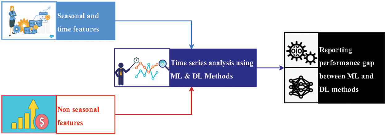
Figure 1: The proposed system block-diagram

In the proposed system, the problem of seasonal goods (e.g., Christmas gifts) price prediction is proposed to be framed as a time series problem. In the proposed system, The ML and DL models are employed to address the problem at hand, for the sake of studying the performance gap between these two approaches. For the ML models, we utilized five models namely, 1) ensemble learning-based models, 2) random forest, 3) Ridge, 4) Lasso, and 5) Linear regression. For the DL models, this research proposes new GRU and LSTM architecture as representative DL models due to their powerful performance in prediction.

In GRU model, as a representative of the recurrent model, the recurrent unit fetches and captures data patterns and dependencies through time spans. A GRU model is composed of a set of cells. Typically, each cell has two gates (i.e., update and reset) and a state vector. Eqs. (1) to (4) illustrate the architecture of a GRU cell.

z(t)=σ(Wzx(t)+Uzh(t−1)+bz) (1)

r(t)=σ(Wrx(t)+Urh(t−1)+br) (2)

o~(t)=tanh(Whx(t)+Uh(h(t−1)⊙rt)+bh) (3)

h(t)=z(t)⊙h(t−1)+(1−z(t))⊙o~(t) (4)

where the hidden state of the previous cell is denoted as h(t−1) and the current input sequence vector is represented by x(t) . Finally, the hidden state ( h(t) ) is the cell output.

The proposed ML model hyperparameters are tuned on the utilized dataset as explained later in this section. For the ensemble learning-based models, this paper proposes the use of Adaboost, Catboost, and bagging methods. Thus, the ML models are examined using two different types of models, classic models, and ensemble models. On the other side, the proposed DL architectures are designed using a distributed asynchronous hyperparameter optimization method, as detailed later in this section. All the proposed models are trained and tested using the hold-out cross-validation technique. Thus, the utilized dataset is split into training and test sets.

3.2 Stacked GRU-DNN Model Architecture

Neural network models are prone to over/under-fitting problems, which are caused by the excessive/less training epochs of the neural network model [35]. Therefore, to prevent the over/under-fitting problems of the DL-based model, one possible solution is to use the early stopping technique [36], which is employed to halt the training when generalization performance starts degrading for a successive number of epochs. For that reason, the training data is split into training and validation groups to track the generalization performance.

Another method to tackle the overfitting problem is to use the dropout method [37]. Dropout is a regularization method that permits training neural networks with different architectures in parallel, where a certain ratio of layer neurons is randomly ignored or dropped out. As shown in Fig. 2, dropout is denoted by the black neurons in the fully connected layers. Adam optimizer [38], which is an adaptive optimization algorithm, is used with its default learning and decay rate settings. Adam optimizer has demonstrated its efficiency in solving practical DL problems, and its results outperform the other stochastic optimization methods. The proposed DL model employs the mean square error (MSE) loss function, given by Eq. (1). That is, given a training data {(Xi,Yi)}i=1N of N observations, the GRU-DNN model is trained with the objective of minimizing the following loss function:

minω⁡1N∑j=1N⁡{‖Yj−F(Xj,ω)‖2} (5)

where ω is the network coefficient, Xi represents the ith the feature vector, Yi represents the ith label, F:IRk→IR1 denotes the neural network flow, and k is the input vector size (i.e., number of lag features).

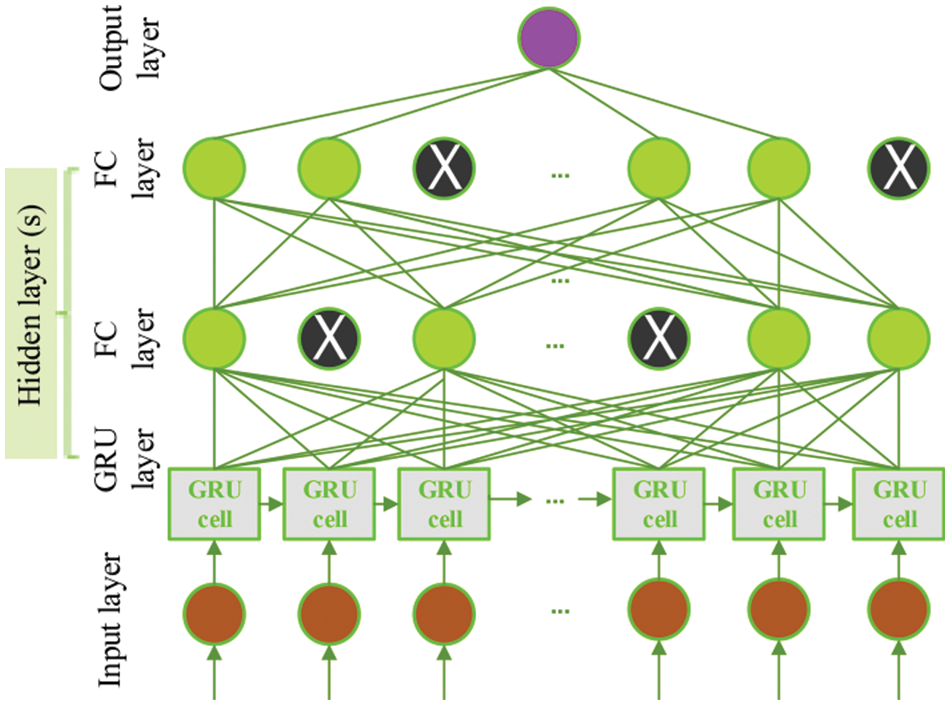
Figure 2: Stacked GRU-DNN model

3.3 GRU-DNN Hyperparameter Optimization

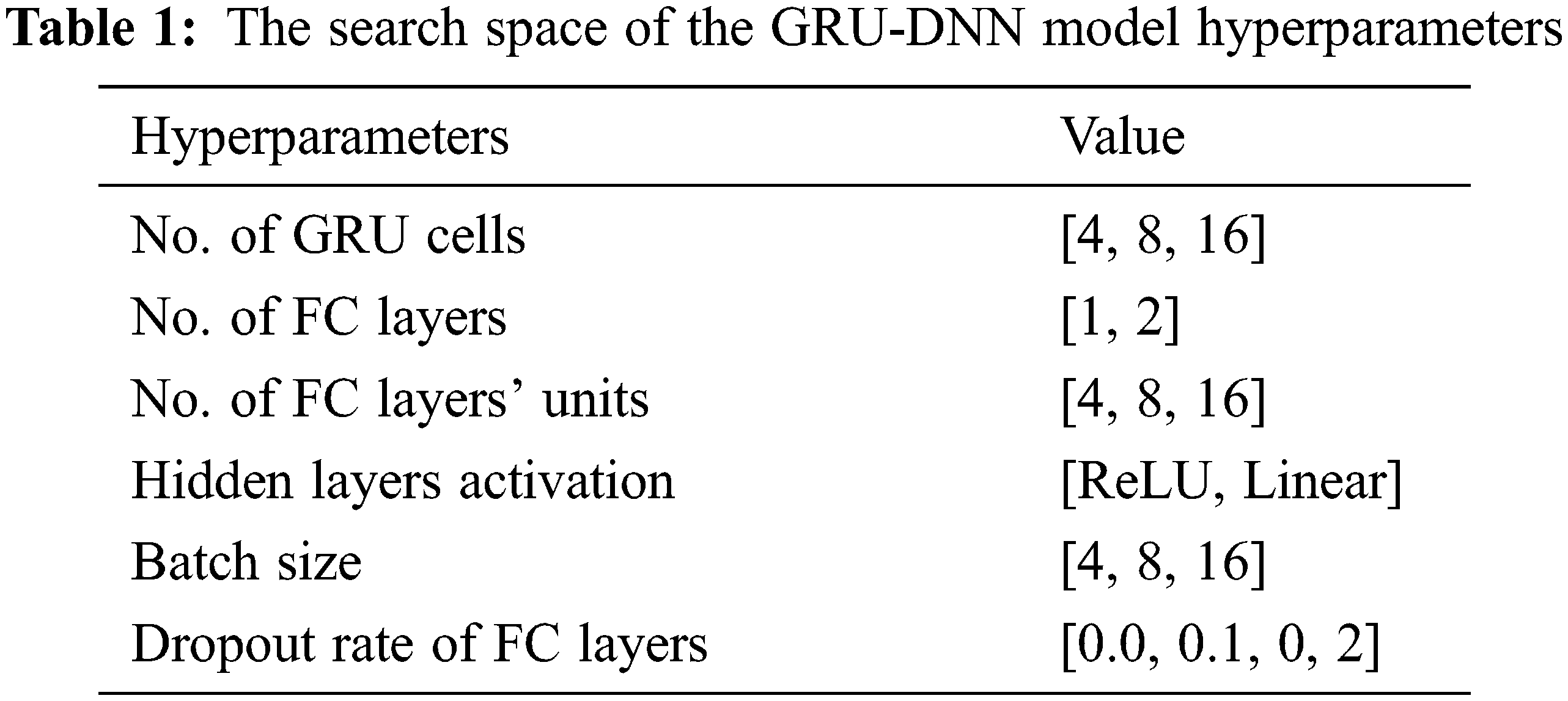
ML algorithms involve the optimization of model hyperparameters. Hyperparameters refer to the model parameters (coefficient) that are used to control the training task. Therefore, such hyperparameters (e.g., number of layers/neurons of a network/layer, learning rate, lag order of ARIMA model, etc.) need careful tuning before the forecasting process. Hyperparameter tuning (or optimization) refers to the process of obtaining the best values for a set of hyperparameters that results in good fitting/generalization of the model. In our proposed work, obtaining the best model hyperparameters is done using a distributed asynchronous hyperparameter optimization method [39]. More specifically, the Tree Parzen Estimator (TPE) [40] method is used in the Hyperopt package1 for parameter searching and optimizing. Table 1 presents GRU-DNN model hyperparameters, and their corresponding search spaces to find the optimal model hyperparameter values.

3.4 Machine Learning Model’s Hyperparameter

Tuning the model’s hyperparameters is one of the most difficult aspects of designing ML models. This is due to the fact that various values for the hyperparameter might produce a wide range of degrees of accuracy. Ensemble learning-based model, Random Forest, Ridge, Lasso, and linear regression are five ML models used in the proposed system. In order to acquire the optimal parameter tuning for each learning model, a grid search is conducted.

For the most part, a grid search is just a series of guesses and checks. The task at hand is to determine which hyperparameter values in the hyperparameter grid will yield the highest cross-validation scores.

Since it is essential to “brute-forcing” all possible combinations, the grid search method is considered to be a very conventional approach to hyperparameter optimization. Cross-validation is then used to assess the models. As expected, the most precise model is the one given the most weight.

The target hyperparameters are initially defined. Once this is completed, the grid search will use cross-validation to try every imaginable setting for each hyperparameter. The hyperparameters are significant since they are one of the most influential factors in the overall behavior of an ML model. Consequently, choosing the optimal hyperparameter values is a crucial objective that decreases the loss function and improves performance. As a result, determining the best hyperparameters values is a critical goal that reduces the loss function and produces better results. Ensemble learning mode Adaboost, for example, adjusts the base_estimator, n_estimator, and learning_rate to achieve the highest accuracy. Grid search, on the other hand, is used in RF to find the best hyperparameters (minimum leaf samples, maximum features, minimum split samples, and the number of estimators). Similarly, the hyperparameter of Ridge and Lasso is alpha.

4  Experimental Results

4.1 Setup

An Intel(R) Core (TM) i7-9750H CPU operating at 2.60 GHz and 16 gigabytes of RAM were utilized in the experiments that were carried out on a computer. The operating system that is being used is Windows 10 64-bit, the Python scripting language, a general-purpose programming language, is used for all of the implementations.

4.2 Dataset

The proposed approach utilizes a dataset of Christmas gifts from an online retailer in order to boost the appeal and value of the products provided. The dataset consists of 18.462 observations and contains significant product information such as the gift type, category, date of arrival in stock, date of stock update, buyer dates, whether the product is on sale or not, price, and the quantity purchased. Other engineered features are extracted from the date feature to represent the time factor of the items.

Using ML and DL methods, the dataset is trained and tested by shuffling and dividing the dataset so that 80% is used for training and the remaining 20% is used for testing. In every method of machine learning, the parameters of the model are configured according to the default settings of the Scikit-learn package.

4.3 Accuracy Metrics

An important component of any suggested system is the evaluation of the ML algorithms that are being used to make decisions. This process is essential for differentiating between classes and getting the best possible classifier. In order to establish the validity of this system, four assessment metrics are employed. One of these measures, the mean absolute error (MAE), is a measure that estimates the average of the difference between the original and predicted values. In this way, it is possible to determine how much the forecasts deviate from the actual information. The following is how MAE is expressed mathematically:

MAE=1N∑i=1N⁡|Yi−Y^i| (6)

Additionally, the MSE is also used to evaluate the precision of regression analyses. MSE is the average of the square of the difference between the actual and anticipated values. The following equation represents MSE

RMSE=1N∑i=1N⁡|Yi−Y^i| (7)

The R2 , which varies from zero to one, indicates how well a model matches the data it represents. Furthermore, it measures how near the actual values are to the regression line. This metric may be calculated using the given equation

R2=1−∑i=1N⁡(Yi−Y^i)2∑i=1N⁡(Yi−Y¯i)2 (8)

The final metric is used to quantify the accuracy of a forecast system is the MAPE. It can be calculated by dividing the average absolute percent inaccuracy by the observed actual values for each time period.

MAPE=1n∑i=1N⁡|Yi−Y^iYi|×100% (9)

where N is the number of observations, Yi denotes the true value, Y^i represents the predicted values, and Y¯i denotes the mean true values.

4.4 Results and Discussion

The evaluation of the proposed models is conducted over three points of comparison, namely, 1) the residual histogram plots, 2) the plots of true vs. the predicted values, and 3) the accuracy metric scores. These three points of comparison should depict the behavior of the proposed predictive models and then the model(s) with the best performance can be recognized visually from the figures and numerically from the accuracy metric scores.

For the first point of comparison, the residual histogram plots should depict the variance of the errors as well as the error ranges. The more the residuals are centered on the value of zero the better the performance of the model is. The less the histogram variance, the better the model is. Figs. 3–5 depict the residuals of the ML models, ensemble learning, and DL models, respectively. The reported residuals of the ensemble learning models (i.e., Fig. 4) are concentrated around the zero values. In comparison to the other two ML and DL models, the ensemble learning models have the highest accuracy rates. The only exception of the ML and DL models is the random forest model. Its performance is the closest to the ensemble learning models-based models. Thus, the residual histograms show that the ensemble learning and the random forest models produced the best performance.

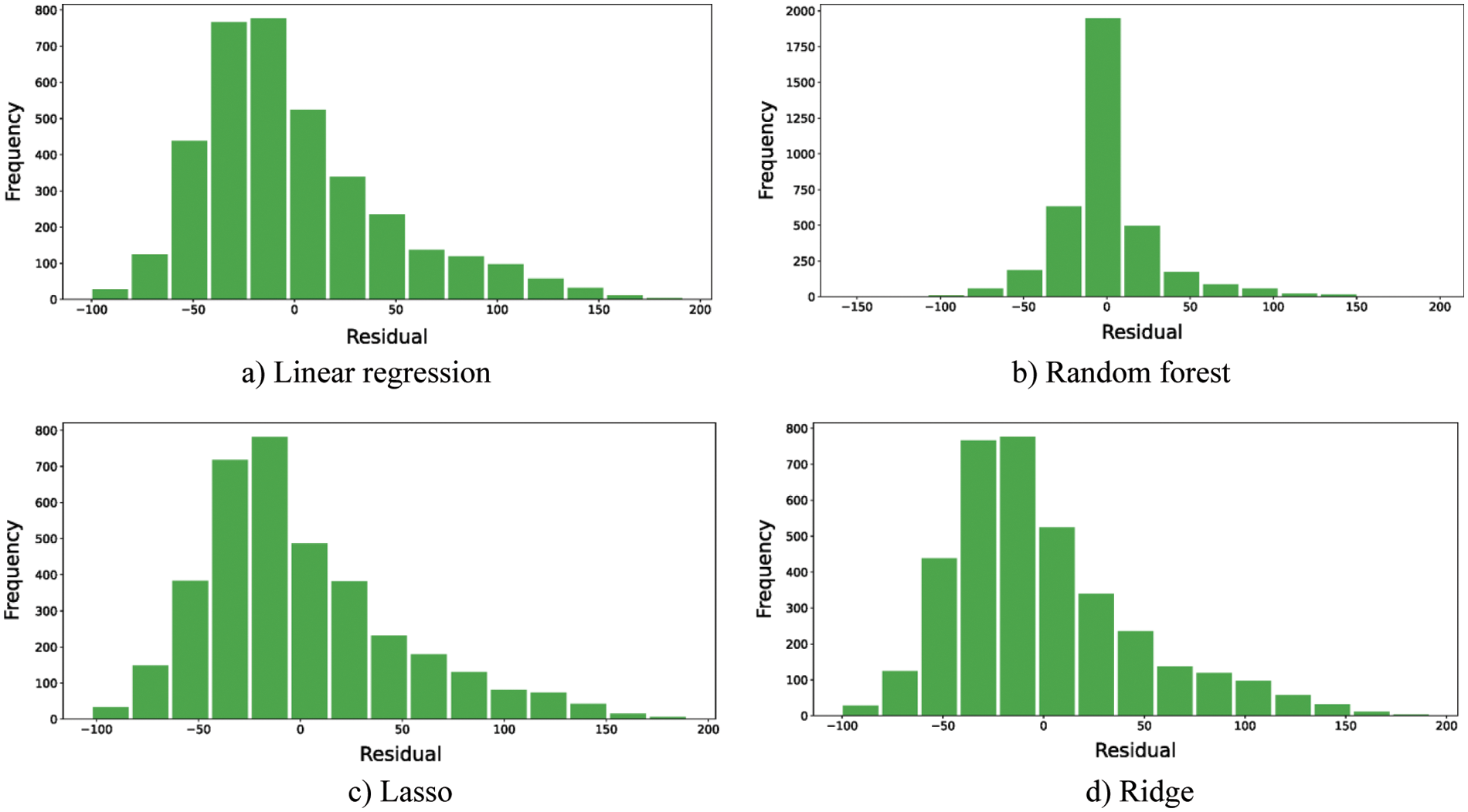
Figure 3: The histogram of residuals for ML models

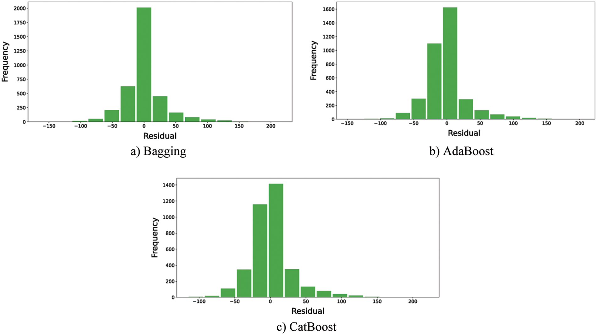
Figure 4: The histogram of residuals for ensemble learning models

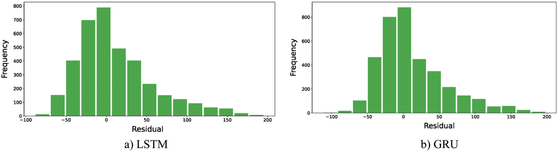
Figure 5: The histogram of residuals for DL models

For the second point of comparison, the true versus predicted values plots are utilized. The predicted value and the true value should be correlated. The more linear are the plotted data, the better the model is and vice versa. In other words, the less deviated the plotted data from the linear equation x=y , the better the model prediction, where x represents the true value, and y represents the predicted value. In predicted against true values, the more linear the depicted shape the better the performance. The predicted prices against the true values are depicted in Figs. 6–8 for the ML models, ensemble learning, and DL models, respectively. Fig. 7 depicted the most linear shape in comparison to the other two figure (i.e., Figs. 6 and 8). In Figs. 7, 7a looks slightly more linear than Figs. 7b and 7c. The model which achieved the highest accuracy was the ensemble-bagging model. Comparing Figs. 6 and 8, it seems that the shape of Fig. 6 is less random than Fig. 8. Thus, the performance of the classic machine learning-based methods was better than the DL-based method on the task of seasonal price prediction.

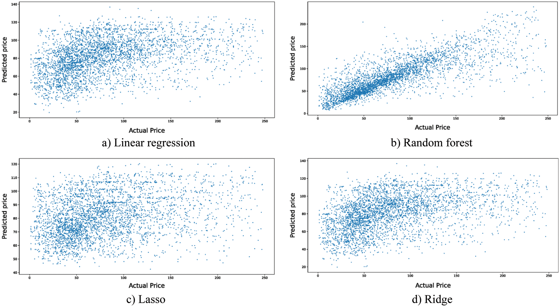
Figure 6: The residuals plot for ML models

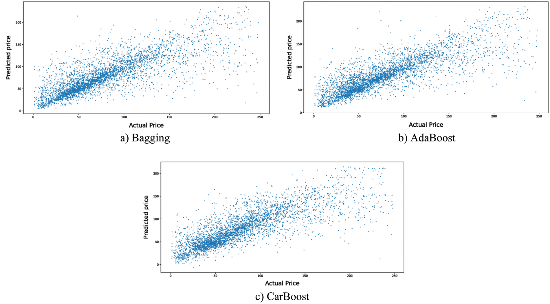
Figure 7: The residuals plot for ensemble learning models

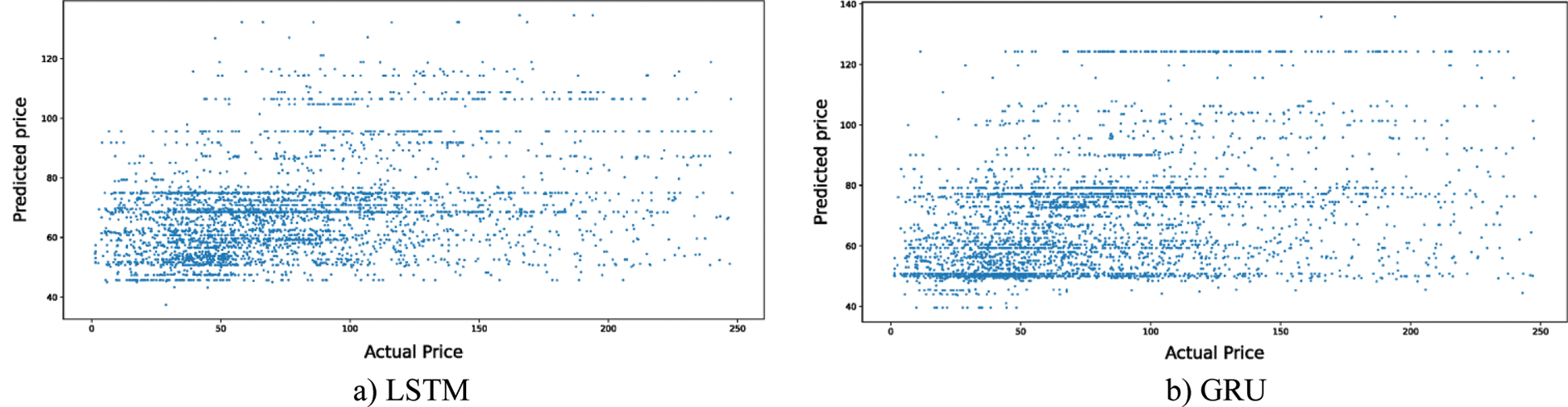
Figure 8: The residuals plot DL models

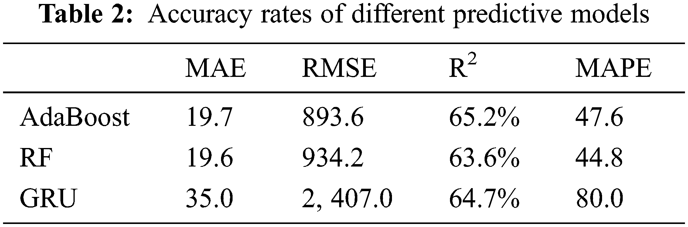
For the last point of comparison, the proposed models’ performances are evaluated numerically using the four accuracy metrics discussed in Section 4.3, namely, 1) MAE, 2) RMSE, 3) R2 and 4) MAPE. The first three accuracy metrics are calculated with the absolute error. In contrast, the fourth accuracy metric reports the error relative to the true values. Table 2 lists the numerical values of one representative model from each approach, namely, 1) the bagging model for the ensemble learning 2) the random forest for the ML models, and 3) the GRU for the DL models. Table 2 shows the performance of these three models on four different accuracy metrics.

Time series data consists of 106 observations for a specific item. Fig. 9 presents item price through 106 time points. The data is split into training set and test set with ratios of 80% and 20%, respectively. The proposed models are trained using training set and evaluated using test set.

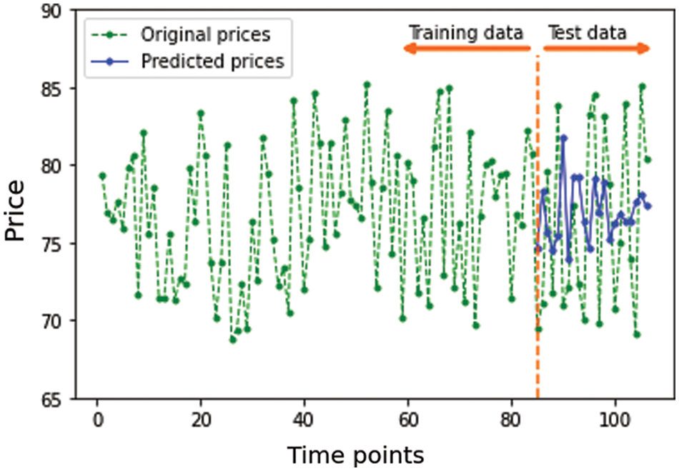
Figure 9: Predictions for a representative seasonal item

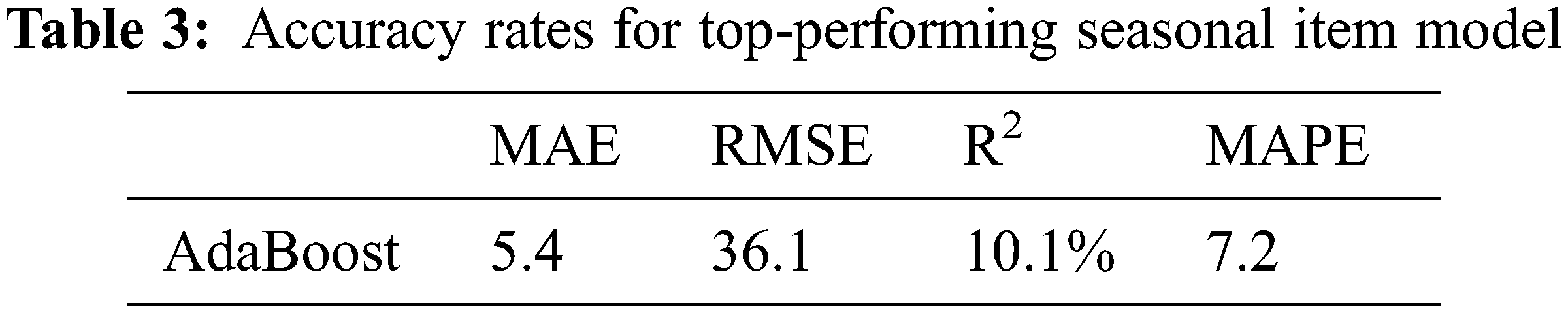
For the accuracy metrics, the top-performing models are the ensemble learning-based model, followed by the random forest model, the DL-based models, and finally the other ML models. The overall results show that the ensemble learning-based models are better than the ML and DL models. Of note, the proposed Adaboost model is the best performing model among all the proposed models followed by the gradient boosting on decision trees model (i.e., CatBoost). Table 3 presents the Adaboost accuracy rates for addressing the seasonal item using the test data, as showed in Fig. 9. The better performance of the ensemble learning models on the problem at hand is that those models benefit from combining the results of several models. The combined models cooperate to find out the patterns of seasonal item prices.

5  Conclusions

This work proposes framing the problem of seasonal item price prediction as a time series analysis task. It addresses the usage of the classic ML models, ensemble learning models, and two proposed DL models. The utilized models were trained and evaluated on a real-life dataset. The obtained results outlined that the ensemble learning models outperformed the classic ML models and DL models on the accuracy metrics. The bagging technique slightly performed better than the Adaboost and Catboost ensemble learning models. Among the classic ML models, only the random forest performance was close to the ensemble learning models. Thus, it can be concluded that the ensemble learning models are the best models to address this problem of price prediction of seasonal times when the problem is framed as a time series problem. The proposed models are tested on a dataset from one source, which is considered the only limitation of this current work; considering several datasets from different sources can better prove the proposed models. The future direction includes exploring the performance of the transformer DL model.

Funding Statement: The authors received no specific funding for this study.

Conflicts of Interest: The authors declare that they have no conflicts of interest to report regarding the present study.

References

1. A. Fathalla, A. Salah, K. Li, K. Li and P. Francesco, “Deep end-to-end learning for price prediction of second-hand items,” Knowledge and Information Systems, vol. 62, no. 12, pp. 4541–4568, 2020. [Google Scholar]
2. Z. Alameer, A. Fathalla, K. Li, H. Ye and Z. Jianhua, “Multistep-ahead forecasting of coal prices using a hybrid deep learning model,” Resources Policy, vol. 65, pp. 101588, 2020. [Google Scholar]
3. P. Yu and X. Yan, “Stock price prediction based on deep neural networks,” Neural Computing and Applications, vol. 32, no. 6, pp. 1609–1628, 2020. [Google Scholar]
4. Y. Li and Y. Pan, “A novel ensemble deep learning model for stock prediction based on stock prices and news,” International Journal of Data Science and Analytics, vol. 13, no. 2, pp. 139–149, 2022. [Google Scholar]
5. M. Nikou, G. Mansourfar and J. Bagherzadeh, “Stock price prediction using deep learning algorithm and its comparison with machine learning algorithms,” Intelligent Systems in Accounting, Finance and Management, vol. 26, no. 4, pp. 164–174, 2019. [Google Scholar]
6. A. Ali, A. Fathalla, A. Salah, M. Bekhit and E. Eldesouky, “Marine data prediction: An evaluation of machine learning, deep learning, and statistical predictive models,” Computational Intelligence and Neuroscience, vol. 2021, pp. 8551167, 2021. [Google Scholar]
7. E. Eldesouky, M. Bekhit, A. Fathalla, A. Salah and A. Ali, “A robust uwsn handover prediction system using ensemble learning,” Sensors, vol. 21, no. 17, pp. 5777, 2021. [Google Scholar]
8. Y. Goldberg, “A primer on neural network models for natural language processing,” Journal of Artificial Intelligence Research, vol. 57, pp. 345–420, 2016. [Google Scholar]
9. D. Amodei, S. Ananthanarayanan, R. Anubhai, J. Bai, E. Battenberg et al., “Deep speech 2: End-to-end speech recognition in English and mandarin,” in International Conference on Machine Learning, New York, NY, USA, pp. 173–182, 2016. [Google Scholar]
10. W. Chan, N. Jaitly, Q. V. Le, O. Vinyals and N. M. Shazeer, “Speech Recognition with Attention-Based Recurrent Neural Networks,” U.S. Patent No. 9,799, 327, Washington, DC: U.S., Pantent and Trademark Office, 2017. [Google Scholar]
11. K. He, X. Zhang, S. Ren and J. Sun, “Deep residual learning for image recognition,” in Proc. of the IEEE Conference on Computer Vision and Pattern Recognition (CVPR), Las Vegas, NV, USA, pp. 770–778, 2016. [Google Scholar]
12. Y. Kim, “Convolutional neural networks for sentence classification,” M.S. dissertation, University of Waterloo, Canda, 2015. [Google Scholar]
13. S. A. Mohamed, A. A. Elsayed, Y. F. Hassan and M. A. Abdou, “Neural machine translation: Past, present, and future,” Neural Computing and Applications, vol. 33, no. 23, pp. 15919–15931, 2021. [Google Scholar]
14. Z. Fan and Y. Wang, “Stock price prediction based on deep reinforcement learning,” in Proc. of the 5th Int. Conf. on Innovative Computing (IC 2022), Guam, pp. 845–852, 2022. [Google Scholar]
15. N. I. Lestari, M. Bekhit, M. A. Mohamed, A. Fathalla and A. Salah, “Machine learning and deep learning for predicting indoor and outdoor IoT temperature monitoring systems,” in Int. Conf. on Internet of Things as a Service-Springer, Sydney, Australia, pp. 185–197, 2022. [Google Scholar]
16. L. Xiao, Y. Zhang, K. Li, B. Liao and Z. Tan, “A novel recurrent neural network and its finite-time solution to time-varying complex matrix inversion,” Neurocomputing, vol. 331, pp. 483–492, 2019. [Google Scholar]
17. C. Chen, K. Li, S. G. Teo, X. Zou, K. Wang et al., “Gated residual recurrent graph neural networks for traffic prediction,” in Proc. of the AAAI Conf. on Artificial Intelligence, Honolulu, Hawaii, USA, vol. 33, no. 10, pp. 485–492, 2019. [Google Scholar]
18. Z. Quan, X. Lin, Z. -J. Wang, Y. Liu, F. Wang et al., “A system for learning atoms based on long short-term memory recurrent neural networks,” in 2018 IEEE Int. Conf. on Bioinformatics and Biomedicine (BIBM), Madrid, Spain, pp. 728–733, 2018. [Google Scholar]
19. S. Ji, J. Kim and H. Im, “A comparative study of bitcoin price prediction using deep learning,” Mathematics, vol. 7, no. 10, pp. 898, 2019. [Google Scholar]
20. D. Alghamdi, F. Alotaibi and J. Rajgopal, “A novel hybrid deep learning model for stock price forecasting,” in Int. Joint Conf. on Neural Networks (IJCNN), Shenzhen, China, pp. 1–8, 2021. [Google Scholar]
21. G. Bathla, “Stock price prediction using LSTM and SVR,” in 2020 Sixth Int. Conf. on Parallel, Distributed and Grid Computing (PDGC), Waknaghat, India, pp. 211–214, 2020. [Google Scholar]
22. Y. -Y. Hong, J. V. Taylar and A. C. Fajardo, “Locational marginal price forecasting using deep learning network optimized by mapping-based genetic algorithm,” IEEE Access, vol. 8, pp. 91975–91988, 2020. [Google Scholar]
23. I. E. Livieris, E. Pintelas and P. Pintelas, “A cnn–lstm model for gold price time-series forecasting,” Neural Computing and Applications, vol. 32, no. 23, pp. 17351–17360, 2020. [Google Scholar]
24. M. A. Mohamed, I. M. El-Henawy and A. Salah, “Price prediction of seasonal items using machine learning and statistical methods,” CMC-Computers Materials & Continua, vol. 70, no. 2, pp. 3473–3489, 2022. [Google Scholar]
25. F. Saâdaoui, “A seasonal feedforward neural network to forecast electricity prices,” Neural Computing and Applications, vol. 28, no. 4, pp. 835–847, 2017. [Google Scholar]
26. C. Naumzik and S. Feuerriegel, “Forecasting electricity prices with ma-chine learning: Predictor sensitivity,” International Journal of Energy Sector Management, vol. 15, no. 1, pp. 157–172, 2020. [Google Scholar]
27. A. Lucas, K. Pegios, E. Kotsakis and D. Clarke, “Price forecasting for the balancing energy market using machine-learning regression,” Energies, vol. 13, no. 20, pp. 5420, 2020. [Google Scholar]
28. T. Xiong, C. Li and Y. Bao, “Seasonal forecasting of agricultural commodity price using a hybrid STL and ELM method: Evidence from the vegetable market in China,” Neurocomputing, vol. 275, pp. 2831–2844, 2018. [Google Scholar]
29. W. Chen, H. Zhang, M. K. Mehlawat and L. Jia, “Mean–variance port-folio optimization using machine learning-based stock price prediction,” Applied Soft Computing, vol. 100, pp. 106943, 2021. [Google Scholar]
30. H. V. Nguyen, M. A. Naeem, N. Wichitaksorn and R. Pears, “A smart system for short-term price prediction using time series models,” Computers & Electrical Engineering, vol. 76, pp. 339–352, 2019. [Google Scholar]
31. M. Al Shehhi and A. Karathanasopoulos, “Forecasting hotel prices in selected Middle East and north Africa region (MENA) cities with new forecasting tools,” Theoretical Economics Letters, vol. 8, no. 9, pp. 1623, 2018. [Google Scholar]
32. M. Al Shehhi and A. Karathanasopoulos, “Forecasting hotel room prices in selected GCC cities using deep learning,” Journal of Hospitality and Tourism Management, vol. 42, pp. 40–50, 2020. [Google Scholar]
33. R. Dharavath and E. Khosla, “Seasonal ARIMA to forecast fruits and vegetable agricultural prices,” in 2019 IEEE Int. Symp. on Smart Electronic Systems (iSES)-Formerly INiS, Rourkela, India, pp. 47–52, 2019. [Google Scholar]
34. S. Aanandhi, S. Akhilaa, V. Vardarajan and M. Sathiyanarayanan, “Cryptocurrency price prediction using time series forecasting (ARIMA),” in 2021 4th Int. Seminar on Research of Information Technology and Intelligent Systems (ISRITI), Yogyakarta, Indonesia, pp. 598–602, 2021. [Google Scholar]
35. S. Geman, E. Bienenstock and R. Doursat, “Neural networks and the bias/variance dilemma,” Neural Computation, vol. 4, no. 1, pp. 1–58, 1992. [Google Scholar]
36. Y. Yao, L. Rosasco, and A. Caponnetto, “On early stopping in gradient descent learning,” Constructive Approximation, vol. 26, no. 2, pp. 289–315, 2007. [Google Scholar]
37. N. Srivastava, G. Hinton, A. Krizhevsky, I. Sutskever and R. Salakhutdinov, “Dropout: A simple way to prevent neural networks from overfitting,” The Journal of Machine Learning Research, vol. 15, no. 1, pp. 1929–1958, 2014. [Google Scholar]
38. D. P. Kingma and J. Ba, “Adam: A method for stochastic optimization,” arXiv preprint arXiv:1412.6980, 2014. [Google Scholar]
39. J. Bergstra, B. Komer, C. Eliasmith, D. Yamins and D. D. Cox, “Hyperopt: A python library for model selection and hyperparameter optimization,” Computational Science & Discovery, vol. 8, no. 1, pp. 014008, 2015. [Google Scholar]
40. J. Bergstra, D. Yamins and D. D. Cox, “Hyperopt: A python library for optimizing the hyperparameters of machine learning algorithms,” in Proc. of the 12th Python in Science Conference, Austin, Texas, USA, vol. 13, pp. 13–20, 2013. [Google Scholar]
Cite This Article
Copyright © 2023 The Author(s). Published by Tech Science Press.
This work is licensed under a Creative Commons Attribution 4.0 International License , which permits unrestricted use, distribution, and reproduction in any medium, provided the original work is properly cited.
Downloads
Citation Tools