A Novel Soft Clustering Method for Detection of Exudates

1  Introduction

In past decades, DR has been a major public health concern and the leading cause of blindness and vision impairment in people with jobs (between the ages of 20 and 60) worldwide. The World Health Organization (WHO) survey predicts that by 2030, there will be 191.0 million people living with DR, up from 126.6 million in 2010 [1]. Therefore, there is a need for early screening and diagnosis for patients with DR signs, as timely detection and treatment in halting the progression of the DR and preventing blindness are essential [2]. In Thailand, the number of patients with DR has been estimated at 4 million people in 2020. According to the statistics, there are 2.3 million cases of blindness and visual impairment. Overall, 100,532 persons are blind, and 2.2 million have low vision [3]. The article also confirms that Thailand has a large number of professional ophthalmologists (approximately 1,300 people) compared to around 4 million people with diabetes mellites is sufficient to provide timely examination and screening for DR complications, especially in rural areas. EXs are one of the essential features of DR. Therefore, it is important to identify EXs early in treating DR. The aim of mass detecting early for EXs complications is to avoid the risk of blindness; 90% of DR-causing blindness can be prevented [4]. Automated detection of retinal images can enhance the effectiveness of detecting programs compared to the manual-based evaluation of EXs, the primary lesions produced on the color retinal surface, which indicate the presence of EXs. EXs appear as bright yellowish pixels on the retina caused by plasma leakage. They are located in the outer layers of the retina and have circular margins [5]. Among DR lesions are EXs on the retinal surface, which are depicted in Fig. 1.

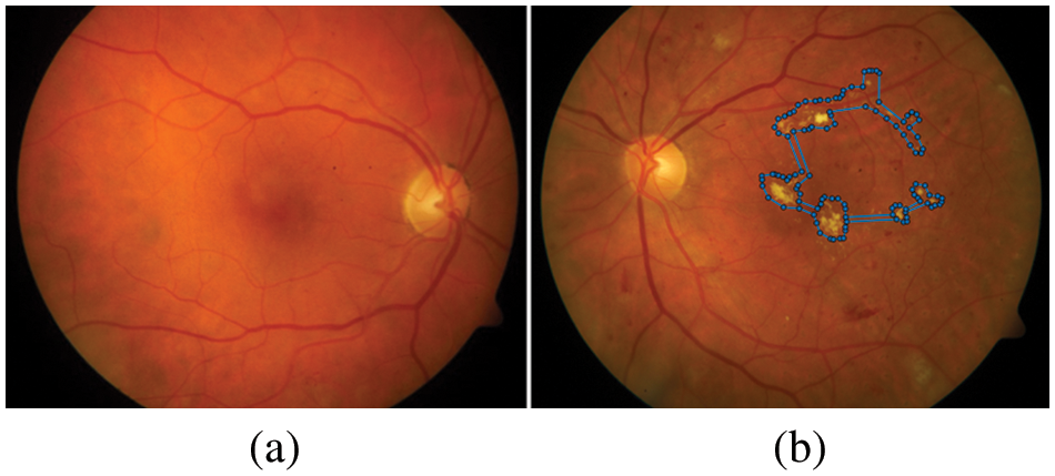
Figure 1: Example of a comparison between the healthy and a retina with DR complications, (a) shows the healthy image, (b) the blue dots represent the retina with the presence of EXs (bright yellowish pixels)

Therefore, the detection of EXs plays an essential and great significance for expert domain knowledge in the early detection of EXs complications [6]. However, a lot of people require retina scans, but expert humans are extremely limited. As a result, the EXs detection method increases the efficacy and accuracy of DR diagnosis while also reducing experts’ workload. This article is organized as follows: Section 2 describes the study approach and reviews previous research relevant to the proposed scheme’s segmentation and detection. Section 3 details the general architecture of the proposed method, and the data preparation for two integrated ways (FHBFCM–NWAS) are described. Section 4 focuses on details of detection analysis compared with referencing the gold standard confirmed by three expert ophthalmologists, the details of three used databases, and setup, it also includes experimental results and compares them with those from other methodologies described in the literature. The conclusion is discussed in Section 5.

2  Related Work

We mainly focus on existing early EXs detection to understand their advantages and disadvantages from 2018 to 2022 to ensure the related work of detection methods used for EXs is as up–to–date as possible. Journals were sourced from ScienceDirect, Institute of Electrical and Electronics Engineers (IEEE) Xplore, PubMed Central (PMC), and Web of Science. The search was “Exudate’s detection” or “Optic disc segmentation” from Quartile score 1 to 4 journals. The search filters were used for keywords and titles. After filtering, machine learning (112 articles) is used to train detection methods. Beyond other methods (89 articles) performs EXs detection without the training stage.

In brief, on the threshold–based segmentation, the studies on the detection of EXs were proposed by Karkuzhali et al. [7]. They showed the intensity variation for the localization center of OD and early detection of EXs. In the study by Rekhi et al. [8], the retinal images were identified as a referable healthy image and EXs image using anisotropic diffusion and adaptive thresholding followed by a Support Vector Machine (SVM) for detection. For the clustering methods, Gao et al. [9] have suggested a combination of improved FCM and Radial Basis Function (RBF) for analysis of EXs illumination. Firstly, the retinal images were classified by improved FCM and then the EXs were grouped by the RBF; as a result, EXs were segmented from retinal images. With the flourishing of the clustering method, some automated EXs detection is proposed by Putra et al. [10]. This research applies a convolutional neural network and mathematical morphology to locate the OD region. Then EXs features were segmented using the adaptive neuro-fuzzy inference system. Qomariah et al. [11] raised for morphological–based segmentation and extracted EXs into two classes: normal and abnormal. The authors just detected the presence of EXs complications using morphological component analysis and the Renyi entropy thresholding. For classification–based methods, some methods have been proposed for detection using SVM and Convolutional Neural Networks (CNN). Some authors, such as Ghosh et al. [12] and Syed et al. [13] adopted SVM for EXs segmentation. With some different ideas, Biswal et al. [14] proposed a new approach for the detection of EXs using an encoder-decoder style network termed “Deep Multitask Capsule Neural Network (M–CapsNet)”. The multilayer perception approaches used by Kusakunniran et al. [15] are only applied to initial seeds identified as having a high probability of being EXs. Huang et al. [16] also used superpixel multi-feature extraction and patch-based deep convolutional neural network to extract from retinal images. Some authors, such as Khojasteh et al. [17] developed fine segmenting and pre-trained CNN for EXs segmentation. Badgujar et al. [18] employed Kirsch’s matrices to remove blood vessels before the detection of EXs with hybrid nature–inspired sequential minimal optimization and boosting ma-chines technique. Fraz et al. [19] introduced an application for only EXs lesions presence. They proposed a morphological reconstruction and Gabor filter to segment EXs candidate lesions. As a result, a combination method achieved good accuracy. On the other hand, the weakness of the morphological reconstruction includes a lengthy computation time if the training set is large. By combining morphological operations, mean shift, normalized cut, and Canny’s edge detector, Banerjee et al. [20] automatically segmented the retinal images of the open-access dataset into EXs or non–referable EXs regions. The retinal image was segmented into referable EXs and non–referable EXs in the Tan et al. study [21]. Adem [22] integrated two methods, circular Hough transforms and CNN to identify three open–access datasets as EXs or non–EXs. Yu et al. [23] built a deep CNN to segment EXs lesions. Kokare [24] segmented EXs and non–EXs using a novel wavelet method. The work by Anitha et al. [25] introduced a way to segment EXs using threshold-based segmentation and CNN from the open–access dataset. Syed et al. [26] integrated a different mixture of features and SVM to segment and detected EXs. Zhou et al. [27] developed a new method using superpixel multi-feature segmentation on two publicly available datasets into EXs or non–EXs. Anggraeni et al. [28] study the performance of the extreme learning machine to detect EXs. In order to segment the features of the EXs, Cincan et al. [29] examined how well the three available pre-trained architectures of CNN, the convolution neural network (SqueezeNet), a residual neural network (ResNet–50), and deep learning (GoogLeNet) performed. Liu et al. [30] classified the DR into referable EXs or non–EXs using a random forest method, the size before the EXs regions, and the local contrast techniques. Using CNN’s deep learning model, Sousa et al. [31] segmented only EXs in DR images. Mohan et al. [32] used the modified speeded–up robust features to detect EXs from DR images. Bharkad et al. [33] segmented EXs lesions in two open–access datasets by integrating the discrete wavelet transform and histogram-based thresholding. The study by Hire et al. [34] used an entire ant colony optimization to segment the EXs in RGB images. After a brief introduction and review of related earlier work, we may state in detail the challenges that must be overcome in order to create such accurate, reliable, and efficient algorithms for the identification of EXs as follows:

•   Most of the works focused on detecting the EXs, which don’t carefully pre-process stages, while noise and poor intensity affect the detection accuracy.

•   The presence of OD deteriorates the performance of EXs segmentation.

•   Under detection of EXs with small regions is considered a challenge due to poor-quality images and invisible regions of EXs.

•   The accuracy of EXs detection decreases on large–scale of retinal images for detection evaluation.

•   All segmentation has not been taken into consideration at the same time; thus, there may be more processing time than it.

Hence, to overcome the existing method’s limitations, we propose a practical three-stage for EXs detection using FHBFCM–NWAS. The following is a brief description of the main contributions of the proposed methods:

•   We have developed a novel fusion method for detecting EXs with different pre–possessing stages, including color normalization, contrast enhancement, noise reduction, and OD removal to pre-process the retinal images. Therefore, in order to successfully detect EXs, a highly effective image processing technique must be applied.

•   We have used a pre-processed image for the training method to a coarse segmentation stage: in the first stage, it analyzed the EXs and structure using a fusion of histogram-based, and in the second stage, it adapts FCM to segment the EXs by removing the region-specific fully connected pixels.

•   To improve the training stage, we have used NWAS and optimal thresholding on fine segmented, which significantly reduces the false positive of performance evaluation and helps to overcome the overfitting regions and small regions for EXs detection.

•   We measured the proposed method on three benchmark open access datasets: DiaretDB0 [35], DiaretDB1 [36], and STARE [37], respectively.

•   The proposed method obtains literature results for detecting EXs compared to the existing method.

3  Proposed Methods

The proposed method for EXs detection is presented in depth in this section. The general architecture of the proposed technique, which includes a description of the training and testing stages to identify EXs, is presented first. Next, we present the detail of the DR dataset and detection performance assessment in the subsequent subsections. Conceptually, the proposed FHBFCM–NWAS is illustrated in Fig. 2. This is a general detection application of EXs by identifying the retinal images into two main categories: healthy images (no apparent EXs) and EXs signs (retinopathy present).

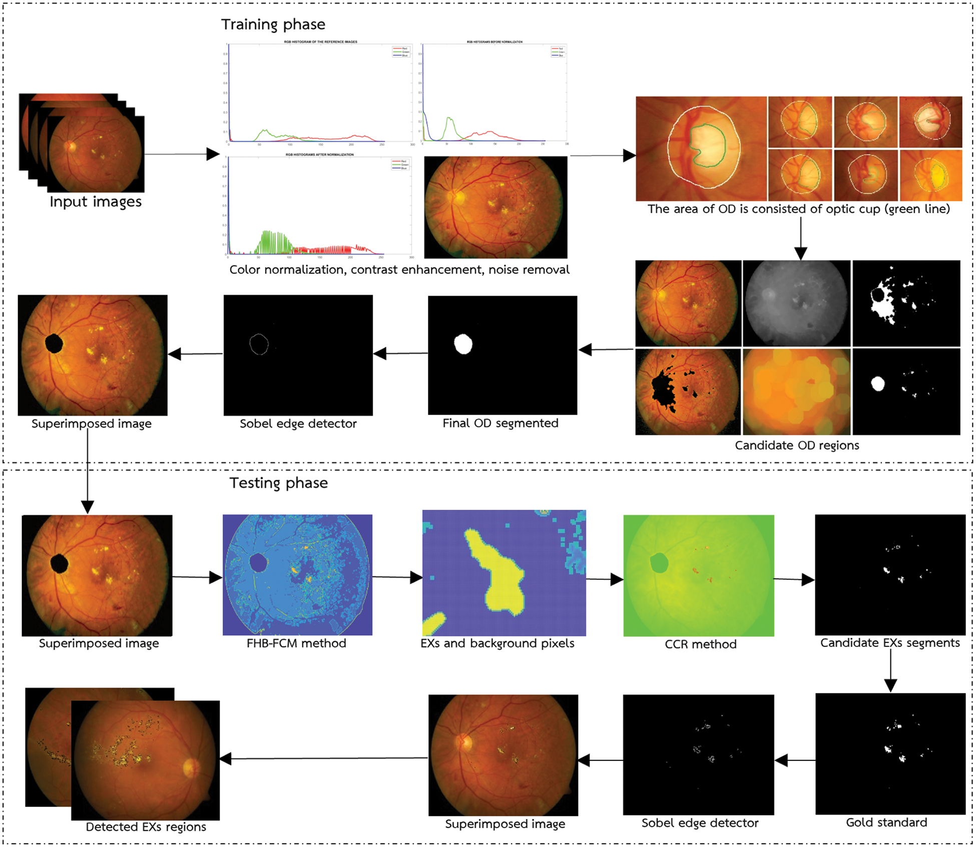
Figure 2: General architecture of the proposed methods

3.1 The Training Stages

The goal of pre-processing input images is to improve the quality of the retinal images for the training task. The training stage can be classified into three categories: image preprocessing, coarse seg-mentation, and fine segmentation. The training stage used in the present work includes color image normalization, noise reduction, contrast enhancement, and OD removal methods. We include the proposed methods in the training stages because there is no apparent difference between the training process and the processing time and cost of the methods. The retinal image should be pre-processed to improve accuracy and the success rate in the EXs detection stage before EXs can be segmented from RGB images. For convenience, we illustrate the procedure step by step in the image pre-processing stages below.

•   Select an excellent retinal image with pixel intensity as a reference. For this reason, the intensity of the original pixel is modified to the current intensity, whereas in the color translation, the intensity pixel contrast of the images is normalized. The histogram specification technique [38] is then applied to modify the values of the histogram of the original retinal image in all datasets to match that of the reference image to improve the image contrast. An application of this method is applied to improve local information in more detail of the original retinal images. Mathematically, for any particular value, the image is adjusted by mapping each pixel with level (xi) in the original image into a corresponding pixel with another grayscale given by the cumulative distribution functions Cinput(xi). This in turn is the desired histogram in the reference image, namely Cdesired(xj). The input image value xi is replaced by xj can be easily calculated from Eq. (1).

Cinput(xi)=Cdesired(xj) (1)

In practice, we use Eq. (1) on every grayscale of the input image (256 images) to get an enhanced image. In the case of an image, this would be a mapping for each of the 256 different states. For retinal images, histogram matching can be used for each color channel independently and mapping can be applied to all RGB channels. To show the qualitative results of histogram matching, the output is given in Fig. 3.

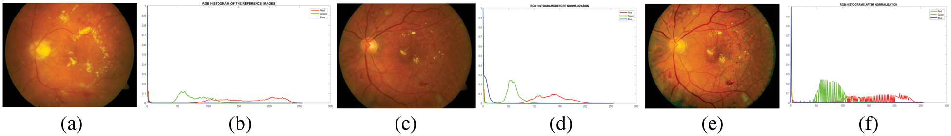
Figure 3: Image and its histogram obtained with contrast adjustment using histogram specification. (a) a reference image, (b) a reference image’s histogram, (c) a poor–quality original image, (d) the image’s histogram, (e) a matched image, and (f) a matched image’s histogram

•   The quality of the normalized image significantly impacts the features of EXs. However, in some images, the intensity is different from the EXs and the background is not very clear due to inadequate intensity near the periphery of the retinal images.

Thus, a local contrast enhancement [39] must be used to improve the separation of subtle variations in each pixel intensity into a more visually discernible distribution. When employing the local contrast technique, the center element is adjusted by shifting the kernel across the image and applying Eq. (2).

Ip=(x,y)=255×(I0(x,y)−Min)/Max−Min (2)

where Ip(x, y) is the color level for the output pixel (x, y) after the contrast stretching process, Io(x, y) is the color level input for data the pixel (x, y), Max is the maximum value for color level in the input image, and Min is the minimum value for color level in the input.

•   It improves the image contrast and noise within the image simultaneously. The noise pixels within these images can cause a wrong in the image segmentation process. Hence, the noise has to be removed by applying the filtration stage before the coarse segmentation. Generally, noise removal from retinal images is based on median filtering [40] without changing the uncorrupted pixel values. Denoising is used to sharpen blurry images, remove noise pixels, or effectively preserve the brightness of the EXs within the image. The median filtering with a 3 × 3 filter is used because they provide excellent noise reduction and preserve EXs details.

•   The removal of OD plays an essential role in segmenting it from other anatomical structures and EXs, as it exhibits similar characteristics to EXs in brightness and contrast. Thus, OD removal helps to prevent false–positive detection of EXs incurred by DR. The loss of small EXs pixels nearer to the OD regions results from this possibly time–consuming procedure. However, there is difficulty in segmenting the OD, as shown in Fig. 4. In this case, detection is difficult due to blood vessel occlusions, abnormal EXs, and imprecise boundaries.

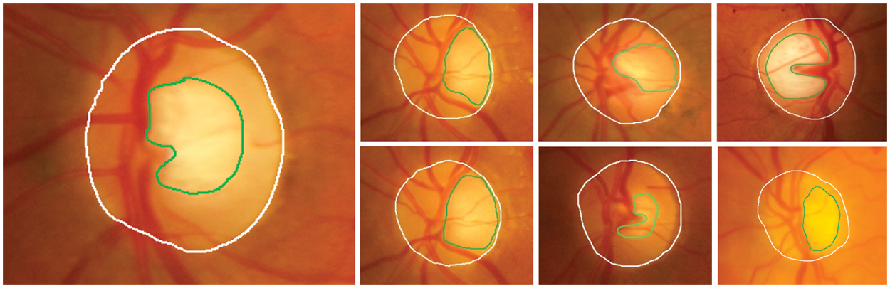
Figure 4: The area of OD (white line) consists of an optic cup (green line); arcs usually segment these features. So, OD removal difficulty is predicting the OD in the retinal images

The OD is a central yellowish area that is an entry point for outgoing blood vessels into the retina, while the Optic Cup (OC) is the brightest region on the OD. The size of OC is about one–third of the OD in healthy images. Therefore, segmenting OD is challenging due to the variations of the OD shape characteristics, size, and intensity. To realize the removal of OD (detecting a region of OD with the highest intensity pixels), mathematical morphology closing [41] is widely used for smoothing the image and removing areas of the blood vessels. In the training stage, we employ structured element learning with a parameter of between 2 and 10 is used to train the method. In the test stage, given an unseen image, the tested method is applied to achieve the segmentation of the OD, and the shape of the structuring element is set to eight by empirical experiments (as demonstrated in Fig. 5b). In the next stage, OTSU’s image thresholding [42] is then performed on the gray image to obtain a binary image and approximation of the boundaries of the OD. The OD boundary represents the frontier between the OD and background regions. In this case, an appropriate thresholding value set to 0.68 will be used (see Fig. 5c). The original image is overlaid with the OD total pixel to identify the OD regions (see Fig. 5d). Here, we assume that the OD regions correspond to the pixels with the most connections. However, the disadvantage of this procedure is that the region with the largest number of connected pixels maybe not always be the region of the actual OD, which in most cases has a smaller area than reality. This is the result of using the previous thresholding values. Therefore, segmenting the region of the OD requires further processing to dilate the area to be more realistic. In this step, we use the method of expanding the area of morphology with an optimal configuration [43] of the structuring element of 7 (see Fig. 5e). Next, the thresholding values with 0.60 are performed again to classify the OD region and create a mask to overlay on the original image (see Fig. 5f). Next, to determine the actual region of the OD, segmentation of the OD was performed using component labeling of connected pixels greater than or equal to 3,200 pixels (established employing all pixels), which can be calculated as in Eq. (3). At this stage, if the number of connected pixels is less than 3,200 pixels, it is not the region of the OD. It will be removed and successfully segmented (see Fig. 5g).

ConnectedRegion=4P(Area)/(Perimeter)2 (3)

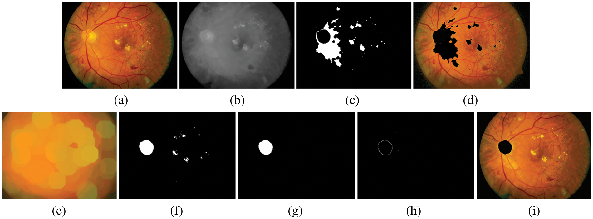
Figure 5: An example of OD segmented. (a) preprocessed image, (b) gray level image, (c) image after applying thresholding method, (d) image of OD candidates, (e) recognition image using mathematical morphology based on dilate operator, (f) image marker with thresholding method again, (g) the OD regions specifically in the connected pixels is more than or equal to 3,600 pixels, (h) image of boundaries of OD after applied Sobel edge detector, (i) internal makers superimposed on the preprocessed image

where ConnectedRegion is the total number of interconnected pixels that are expected to be the region of the OD, Area is the total amount of pixels in the OD region, whereas Perimeter is the total number of pixels along the OD’s perimeter (Perimeter = 2π(radius/2)) [44]. Thus, the binary mask of OD regions is obtained by cleaning as per Eq. (3). OD detection is done in this stage. Finally, an image of the boundaries of OD after applying the Sobel edge detector (see Fig. 5h) and internal makers are superimposed on the preprocessed image (see Fig. 5i). The proposed method’s performance was evaluated by an overlapping score of actual OD pixels and segmented region by the method [45]. The performance analysis of the calculated OD region can be defined as per Eq. (4).

Score=Area(Trueregion∩Sengmentedregion)/Area(Trueregion∪Sengmentedregion) (4)

Where Score represents the overlapping value to measure the area between ground truth pixels and segmented result pixels, Trueregion represents the set of pixels that represent the true OD contours in the gold standard, and Segmentedregion is the set of pixels that represent the segmented results. In this respect, to point out the accuracy of overlapping the OD segmented is 92.85% (65 out of the 70 images), 92.30% (48 out of the 62 images), and 92.30% (12 out of the 13 images) on DiaretdB0, DiaretdB1 and STARE, respectively.

3.2 Color Histogram–Based Segmentation

To extract the features of EXs from the preprocessed image, a coarse segmentation is often performed after the pre-processing processes have been completed. The Region of Interest (ROI) was selected from the RGB space and a histogram analysis technique was performed for the segmentation of EXs.

i) In a color histogram-based method [46], a color histogram peak frequently represents an area of uniform color. Hence, the EXs features and non–EXs (background) of the RGB images can separate by finding the peak of the color histogram and selecting the appropriate thresholding. Note: the color histogram analysis is unsuitable for the image corrupted by noise. The RGB color component of the color histogram is quantified, and a level in the range [0,255] is obtained. Mathematically, let Xi is the ith vector and also the number of ith color pixels. So, s(i)=xi , where 0≤i≤255. The peak finding in the color histogram can be defined as follows:

•   Create a new histogram curve as per Eq. (5).

Ts(i)=s(i−2)+s(i−1)+s(i)+s(i+1)+s(i+2)5 (5)

where s represents the RBG color components and 2≤i≤L−3. Based on segmentation done using the color retinal image, the half window size can be set from 2 to 5 in this work.

•   Identify all peaks finding algorithms as per Eq. (6).

Ps=((i,Ts(i))|Ts(i)>Ts(i−1)andTs(i)>Ts(i+1)) (6)

where Ps is the set of peaks and can be replaced by RGB color space. The set of peaks segmented from Ts(i) and 1≤i≤L−2.

•   Identify all valleys finding algorithms by using Eq. (7).

Vs=((i,Ts(i))|Ts(i)<Ts(i−1)andTs(i)<Ts(i+1)) (7)

where Vs is the valleys segmented and can be replaced by RGB and 1≤i≤L−2.

•   Using Eq. (8), remove all peaks and troughs based on the fuzzy rule-based approach.

IF(i is Peak) AND (Ts(i+1)>(Ts(i−1)) THEN (Ts(i)=(Ts(i+1))IF(i is Peak) AND (Ts(i+1)<(Ts(i−1)) THEN (Ts(i)=(Ts(i−1))IF(i is Valley) AND (Ts(i+1)>(Ts(i−1)) THEN (Ts(i)=(Ts(i−1))IF(i is Valley) AND (Ts(i+1)<(Ts(i−1)) THEN (Ts(i)=(Ts(i+1)) (8)

where s can be replaced by RGB and 1≤i≤L−2. Identify the peaks of a salient color by the turning point with positive to negative the number of pixels greater than the set Thresholding (T). The typical value for T is set to be 123 based on the retinal image segmentation. The cluster centroids are removed to reduce the number of pixels assigned to the cluster centroids under a thresholding V. Where N is the total number of pixels in the color image, the value for V is set to 0.005–0.006 N.

ii) The following Eq. (9) determines the distance between any two cluster centroids for the RGB color component.

D(cj,ck)=(Rj−Rk)2+(Gj−Gk)2+(Bj−Bk)2,∀j≠k, (9)

where 1≤j≤M and 1≤k≤M while Rj, Gj, and Bj are the value of the RGB color component of the jth cluster centroid, and Rk, Gk, and Bk are the value of the RGB color component of the kth cluster centroid, respectively. Based on analysis done using RGB color component, D (distance between any two cluster centroids) normally is 24.

3.3 Pixel Grouping by FCM

The change in distance is determined along the average change between peaks after the RGB color histogram has been examined. The clustering approach uses peak points above the average to determine the initial values of clusters, and the FCM was given the number of peaks [47]. The clustering method groups the bright yellowish pixels in the EXs and the pixels in non–EXs as different as possible. The initialization condition is affected by the number of cluster centroids, and the clustering centroids’ locations also affect the accuracy of the detected image. The proposed suitable cluster centroid for grouping the bright yellowish pixels as a cluster by using FCM and the objective function Jm of the FCM is expressed as per Eq. (10).

Jm(U,v1,...,vc)=∑j=1N∑i=1C(uij)m‖di−vj‖A2 (10)

where U denotes the fuzzy C–partition, v1,…,vc denotes the vectors of centers, C denotes the number of clusters, N denotes the total number of sample feature vectors, uij denotes the degree of membership of the i pixels to the j cluster centroid, di denotes the dimensions of the sample vectors, vj denotes the vector center of cluster j, and m denotes the exponential weighting and ||∙||A represent A–norm of data with the center between the di and vj data pixel. The squared distance between di and vj shown in Eq. (11) is computed in the A–norm as per Eq. (11).

dij2=‖di−vj‖A2=(di−vj)TA(di−vj). (11)

With these observations, we can decompose Jm into its basic elements to see what property of the points (di) is defined as per Eqs. (12a–12d).

dij2=squared A−distance from point  di to the center of vj (12a)

(uij)mdij2= squared A −error incurred by representing di by vjweighted by the membership of di in cluster j. (12b)

∑i=1C(uij)mdij2= sum of squared A - error due to di partial replacement by all c of the centers (di) (12c)

∑j=1N∑i=1C(uij)mdij2=overall weighted sum of gerneralized; A− errors due to replacing d by v.  (12d)

Where uij is the degree of membership, C is the number of clusters, and N is the total number of sample features. FCM uses the iterative optimization method to improve the membership function. Initial M clustering centroids are chosen at random, and the initial value of the iteration number is 1. The new membership degree with updated fuzzy membership of membership degree matrix uij is calculated as Eqs. (13) and (14), respectively.

uij = 1∑k=1M(dijdjk)2/(m−1) (13)

where 1≤i≤N,1≤j≤M. If dij = 0, then uij = 1.

cj =∑i=1N(uij)mdi/∑i=1N(uij)m (14)

This process stops when Eq. (15) is defined, and some iterations are reached.

maxij(|uij(k+1)−uij(k)|)<T (15)

Where T is a termination criterion, k is the iteration number. The input to the FCM is a set of features. In this subsection, the 512 × 512 retinal image is used to demonstrate the effectiveness of the FHBFCM. For Figs. 6b–6d, after applying the peak finding method, the color histogram has two dominating peaks (EXs and background pixels). Therefore, the number of dominant peaks is set to 2. The EXs and background images are separate from the FCM. Centroids for the clusters are 15, 20, and 25, respectively.

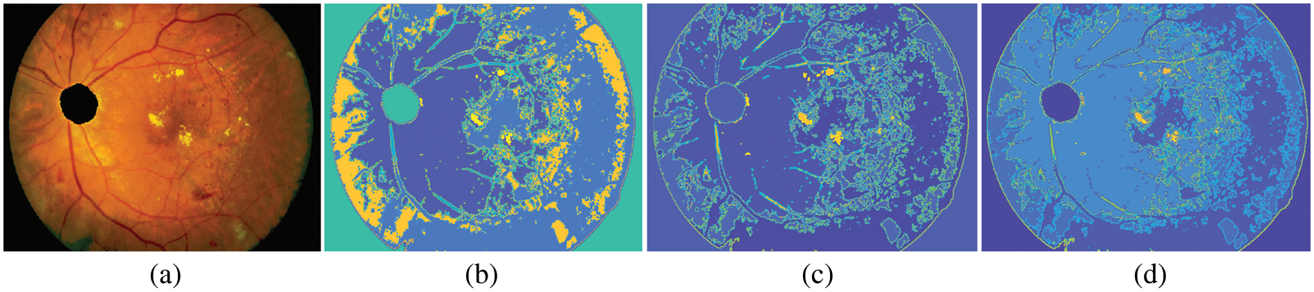
Figure 6: Example of FHBFCM, (a) input pre-processed image, (b)–(d) segmentation results associated with FHB with bins = 2, window size = 3, and final detection map using FCM of the FHB with cluster = 15, 20, and 25 in RGB color space

3.4 Color Representation Using NWAS

This section describes how EXs are detected using color information and representations based on NWAS. However, it is challenging to segment EXs from the background because they are associated with other diseases with similar color and pixel information of lesions. The lesions of all EXs appear as bright yellowish pixels and are brighter than in other regions. Therefore, all EXs pixels are assigned as one class. In some cases, if the evidence of the combining methods is erroneous, the final decision is made by three expert ophthalmologists.

In this stage, the color information of the RGB image is segmented into bright yellowish and dark pixels. Candidate EXs (abnormal) are segmented from bright yellowish pixels, while candidate background (healthy image) is segmented from dark pixels. Finding EXs is an essential task since the color intensity allows the use of color component representation over the surface of the whole image. For candidate bright yellowish pixels (EXs) searching, the yellowish pixels are selected directly as candidate EXs since the OD was removed in the preprocessing stages. We can estimate a pixel value from a window of 3 × 3 with a linear combination of eight neighboring pixels to the central pixel. Fig. 7c shows the cluster representation with a window of a 3 × 3 matrix, which could represent any of the RGB color components.

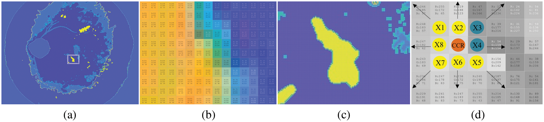
Figure 7: Pixel–by–pixel features selection by color component analysis. (a) EXs lesions segmentation using FHBFCM, (b) EXs and background color information, (c) the pixels of EXs and background region, and (d) selected pixels with size 3 × 3 in RGB color spaces

It affected the detection of FHBFCM in the previous section (see Fig. 7a), so a need to modify it more efficiently to reduce false–positive scores. Here, NWAS is the center pixel, and X1,…,X8 are the eight neighboring pixel values. Respectively, if all the pixels in the region are brighter than any pixel outside the region, that region is considered an EXs. Since maximum and minimum pixel values are searched in the proposed method, the estimate of the NWAS can be computed as the average of the eight neighboring pixel values. Mathematically it is defined as Eq. (16).

NWAS=19∑i=19Xi (16)

The middle pixel is not used for calculations, which makes it possible that the region does not have to be circular. It is also possible to represent NWAS by the median of the eight neighbours, which is computed by ordering the Xi in numerical order and taking the mean of the two middlemost values since there is an even number of neighbours. In Fig. 7c, the pixels X1, X2,…, X9 can be considered neighbours of NWAS. Then, the method by which to calculate the value of NWAS is to perform a linear regression technique over the entire image, which would be to find the constants, X1(r0, g0, b0), X2(r1, g1, b1),…, X9(r8, g8, b8), which best fit by as Eq. (17) for all of the possible 3 × 3 matrices in the image.

NWAS=X1(r0,g0,b0)+X2(r1,g1,b1),...,+X9(r8,g8,b8) (17)

Then we use the linear equation obtained to calculate NWAS for each 3×3 metric individually. Methods of incorporating the matrix of an image have been described, referred to as mean value for cluster center representation, where RGB values are produced by using one of the matrix transformations. The NWAS is done by calculating each RGB color component using Eq. (18) and detecting EXs using a single–color component value represented in Algorithm 1.

R={BG if R≤232EXs if R>233,G={BG if G≤178EXs if G>179,B={BG if G≤82EXs if G>83 (18)

where R, G, and B represent the contained intensity information inside the RGB color component and BG is the background region. After calculating the color components of each pixel in the retinal images into relative values, EXs detection can be classified using optimal thresholding. Fig. 8 shows some examples of detecting for EXs (bright yellowish pixels). A selected bright yellowish pixel belonging to the EXs has relative color values of 233, 179, and 83 in the relative RGB color components, respectively. Next, each of the relative color components is classified by single thresholding. EXs pixels within range [0.68,1], [0,0.1], and [0,0.1] are selected in the relative RGB spaces respectively. Finally, the segment thresholding results are integrated with the Sobel edge operator.

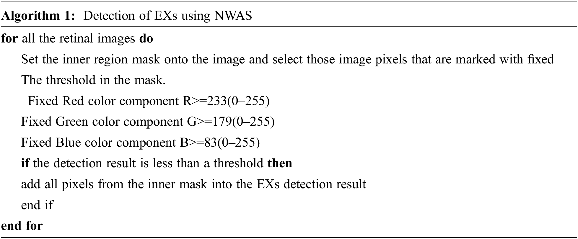
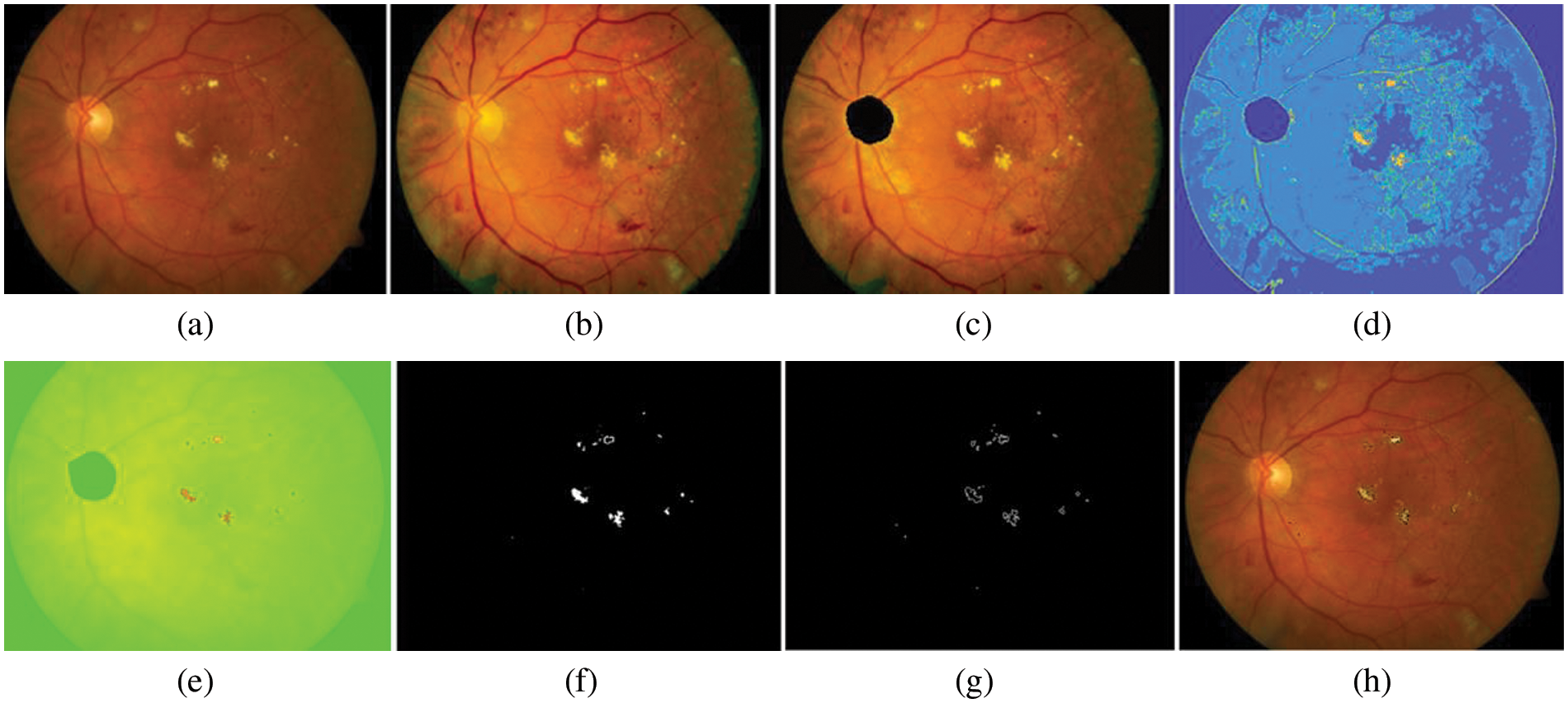
Figure 8: EXs detected image. (a) original retinal image, (b) histogram matched image, (c) OD detected, (d) segmentation map using FHB with bin = 2, window size = 3, and cluster = 25, (e) EXs detected using NWAS with R = 233, G = 179, and B = 83, (f) EXs marker with thresholding method, (g) image of boundaries of EXs after applied Sobel edge detector, (h) EXs detected superimposed on the original retinal image

3.5 Testing Phase and Evaluation of Detection Results

After the training phase is evolved, we use it to identify several EXs pixels of test images in the testing phase. Based on this, manual segmentation by three ophthalmologists from three different hospitals is used to compare the proposed method results based on the provided gold standard images. To evaluate the proposed method’s performance in detecting EXs across three different datasets that are available publicly, the set of three estimation parameters was used to conduct statistical comparisons of Sensitivity (SEN), Specificity (SPEC), and accuracy (ACC). SEN is a statistic for calculating the percentage of correctly identified EXs to all EXs. In contrast, SPEC calculates the percentage of non–EXs pixels wrongly identified as non–EXs pixels in detection. ACC is the total of all correctly identified EXs and non–EXs divided by the total amount of EXs pixels. The better the detection, the higher the value. Results required in SEN, SPEC, and ACC calculations, True Negative (TN) means that the image is non–EXs and the method also detected it as non–EXs, and True Positive (TP) represents the image showing EXs and was correctly detected as having EXs, False Negative (FN) is the procedure detected EXs are as non–EXs, but it is EXs, and False Positive (FP) means that the image is non–EXs, but the method detected it as EXs. The formula to calculate the SEN, SPEC, and ACC as explained above can be calculated as per Eqs. (19)–(21), respectively [48,49].

Sensitivity(SEN)= (TP/TP+FN) × 100 (19)

Specificity(SPEC)= (TN/TN+FP) × 100 (20)

Accuracy(ACC)= (TN+TP/TN+TP+FN+FP) × 100 (21)

Comparison with other detection methods for EXs. To our best knowledge, there is still limited detection of EXs with a specific goal on EXs lesions. We also attempted the above detection method to compare the beat detection performance by adopting the “SEN”, “SPEC”, and “ACC” values.

4  Data and Experimental Results

In this study, we test the effectiveness of EXs detection using several open-access datasets. Some of the best–known open–access datasets that contain retinal images for training and testing the proposed approach are DiaretDB0 [50], DiaretDB1 [51], and STARE [52]. There are 130 images in the first testing set (DiaretDB0), 20 of which are healthy, and the other 110 showing signs of EXs. In order to train the methods using the gold standard images as references, a data set of 26 images was used. The remaining 104 images were used to test the approaches. The second testing set (DiaretdB1) includes 89 images; 84 images correspond to signs of the EXs and 5 images do not show any sign of EXs. Expert ophthalmologists manually label these images. In this way, we divided the total number of images into 70 for testing and 19 for training. Another dataset of retinal images can be obtained in the third set, the SATRE project, done by Dr. Michael Goldbaum at the University of California, San Diego, and supported by the American National Institutes of Health. This set includes a diagnosis for each of the 400 images and a list of diagnosis codes, which can be obtained from STARE. In this way, we divided the total number of images into 340 for testing and 60 for training.

4.1 Set Up and Experimental Results

In the following section, we have considered an FHBFCM to perform detection with color retinal image resized of 512 × 512 sub-image with the following parameters: the size of the windowing process used to compute the color information from a histogram–based is set to be 3 × 3 neighborhood for all of the location. The number of bins for coarse segmenting is set to 2. Several parameters of FCM will be given for several values (comprised between 3 and 25) of C, and the number of classes of the final fused segmentation map with the cluster is set to 25. Finally, we use R = 233, G = 179, and B = 83 segmentations provided by using NWAS of the color component RGB. The final result of the detection is shown in Fig. 9, where they found EXs are superimposed on the intensity of RGB spaces. The result can also be used as a screening system for EXs. The proposed method has enormous performance excellence over the DiaretdB0, DiaretdB1, and STARE with SEN, SPEC, and ACC, as shown in Table 1.

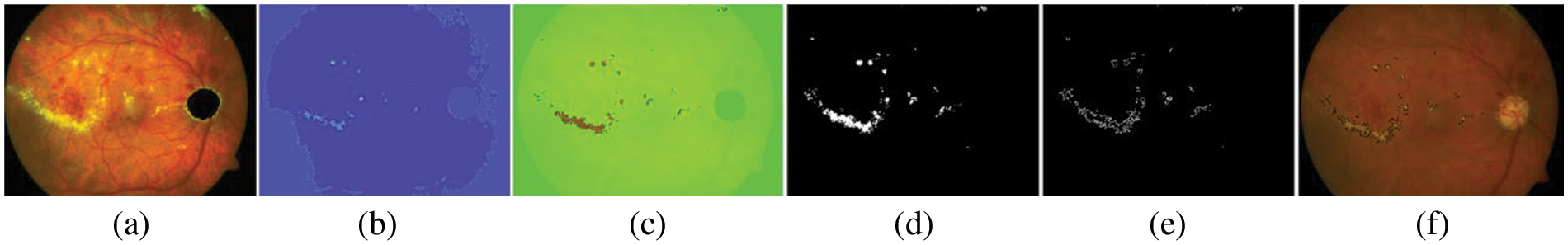
Figure 9: Results of EXs segmentation on open–access datasets as a testing set, (a) pre-processed image, (b) after applying the proposed peak finding method, (c) detected image using NWAS, (d) retinal images have been marked into EXs and non–EXs by thresholding, (e) EXs and boundaries to set to make it on the original image, (f) EXs detected an image superimposed on the original image

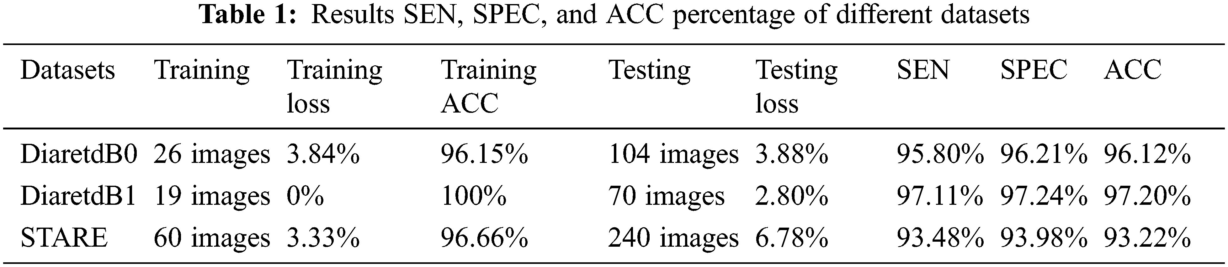
We divided Table 1 into three parts according to three open–access datasets. The proposed method was calculated using Eqs. (19)–(21). The EXs detection with DiaretdB0 as a validation set gives 3.84% training loss, 96.15% training accuracy, 3.88% testing loss, 95.80% SEN, 96.21% SPEC, and 96.12% ACC for the experiments. At the same time, in DiaretdB1, the methods show improved results over the previous dataset with correspondingly the training loss, training accuracy, testing loss, SEN, SPEC, and ACC scores of 0%, 100%, 2.80%, 97.11%, 97.24%, and 97.20%, respectively. In comparison, the methods obtained the training loss, training accuracy, testing loss, SEN, SPEC, and ACC scores of 3.33%, 96.66%, 6.78%, 93.48%, 93.98%, and 93.22% in STARE. It is also noted that the methods have reached a competitive result with the highest ACC of 97.20% in DiaretdB1. The reason for the low SEN score in EXs detection is that there were relatively many retinal images that contained a few small yellowish dots that were often very difficult to distinguish with the expert ophthalmologist, which caused the miss–detection. However, the accuracy of EXs detection seemed to be good since EXs pixels were accurately segmented as EXs with high SPEC scores and other pixels as non–EXs. Some of the EXs are marked by three expert ophthalmologists and the image with relatively small EXs not detected by the proposed methods from STARE is shown in Fig. 10.

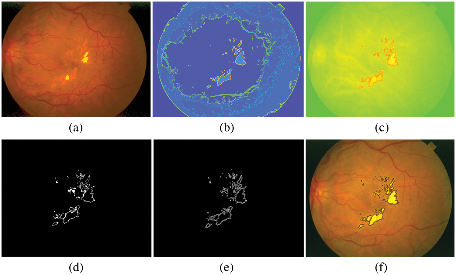
Figure 10: Results of EXs detection on STARE as a testing set, (a) pre-processed image, (b) after applying FHBFCM, (c) detected image using NWAS, (d) image after applying thresholding, (e) EXs boundaries by Sobel edge detector, (f) EXs detected image superimposed on the original image

4.2 Comparison with Related Work

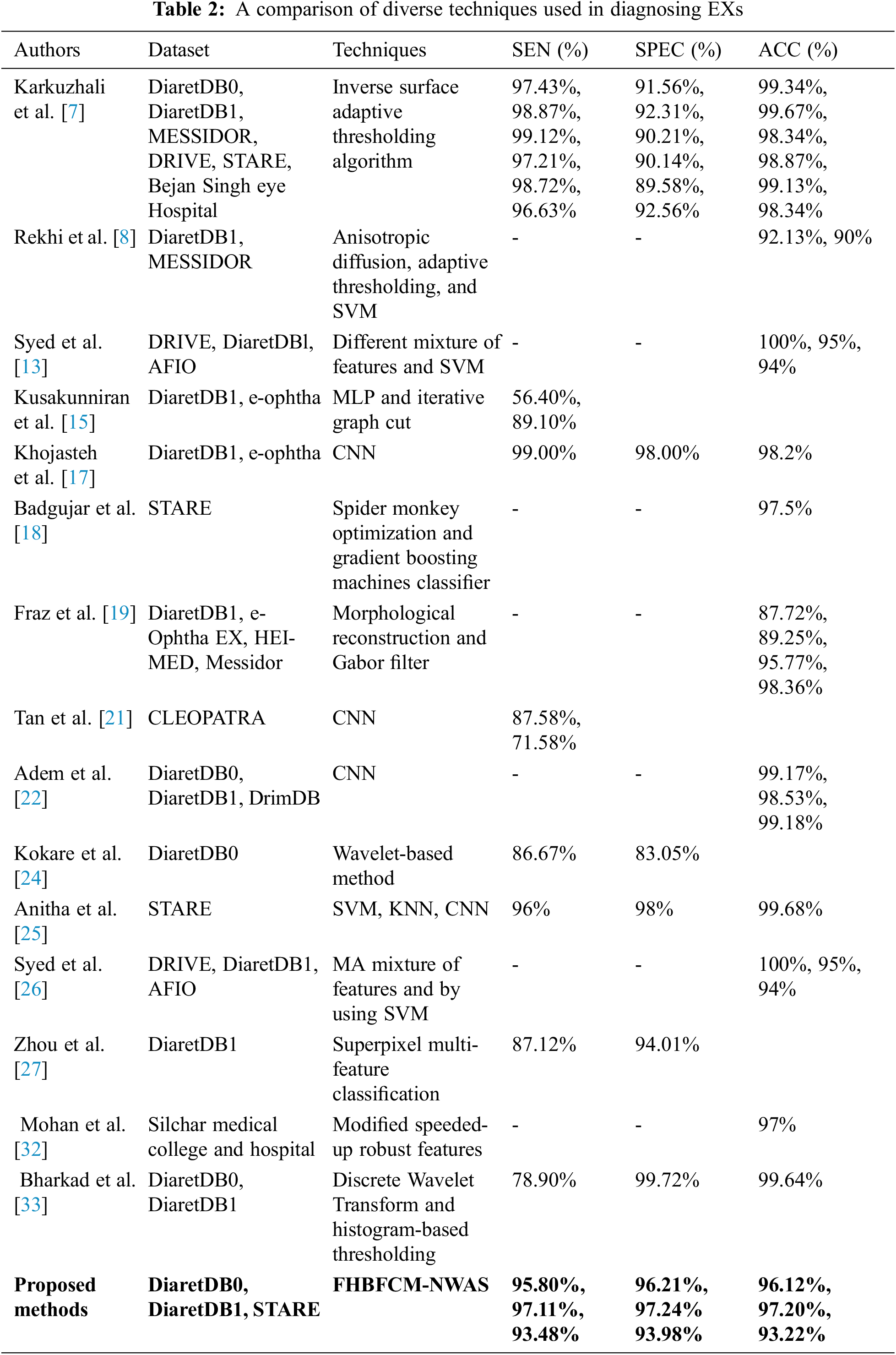
These subsections list the EXs detection, and their experimental results explained in the related work. Karkuzhali et al. [7] developed methods for the detection of EXs. The study is based on many retinal images from DiaretDB0 for testing and reports relatively good experimental results. SEN was 97.43%, SPEC was 91.56%, and ACC was 99.34%, respectively. Khojasteh et al. [17] have used CNN method for detecting EXs. They reported 99.00% SEN, 98.00% SPEC, and 98.20% ACC for detecting EXs. Anitha et al. [25] proposed the combination of SVM, K–Nearest Neighbor (KNN), and CNN to identify the EXs. They report 96.00% SEN, 98.00% SPEC, and 99.68% ACC, respectively. Bharkad et al. [33] have proposed discrete wavelet transform and histogram-based thresholding that can identify EXs in 89 images. They reported 78.90% SEN, 99.72% SPEC, and 99.64% ACC, but they did not mention using the retinal image for testing. The comparison of the proposed method’s segmentation results with the existing literature is shown in Table 2.

4.3 Running Time

The running time impedes the FHBFCM–NWAS and the proposed method is not a particular case. The experiments are run using the MATLAB 2020a programming environment on a personal computer with an Intel (R) Core (TM) i7–6700 K, Central Processing Unit (CPU) running at 4.0 GHz, 512 Gigabyte (GB) of Solid State Drive memory, and 16 GB of RAM. The proposed method requires less running time than competing strategies. In the coarse segmentation stage by using histogram-based, processing one image took around 6 s, including pre-processing, and candidate the EXs, where the grouping of the bright yellowish pixels as a cluster by FCM takes less than 2 s (4 clusters) to 6 seconds (12 clusters) due to the varying number of clusters in the test image. In the EXs detection by using NWAS, another 4 s are spent to get the final EXs detection. It takes less than 1 second on average for boundaries detection results. Overall, it takes 13 s per image to detect EXs in RGB images. The proposed automated EXs detection is a flexible method for DR detection due to its demonstrated effectiveness, robustness, and fast execution. However, the computational efficiency of coarse segmentation may be further improved using other clustering methods since this task can be well integrated. Careful image pre-processing stages can alleviate the high computing time in the coarse to fine segmentation stage.

5  Conclusions

This paper proposed a novel soft computing method called FHBFCM-NWAS for accurate EXs extraction that is important to classify DR features to human eyes. An improved FHBFCM by NWAS and a set of four selected features from stages of pre-processing to evolve the detection method is proposed. The features of DR train the optimal parameter of FHBFCM for detecting EXs diseases through a stepwise enhancement method through the coarse segmentation stage. The histogram function is applied to find the color intensity in each pixel and performed to accomplish RGB information. This RGB information is used as the initial cluster centers for creating the appropriate region and generating the homogeneous regions by FCM. Afterward, the best expression of NWAS is used for the delicate detection stage.

To confirm the effectiveness of the proposed FHBFCM–NWAS for EXs detection, we compared FHBFCM–NWAS with the existing methods using three publicly available datasets. SEN, SPEC, and ACC were measured for comparative analysis. According to comparative analysis, SEN, SPEC, and ACC accuracies were 97.11%, 97.24%, and 97.20% for DiaretdB1. We can use these methods to assist experts in classifying retinal images into EX and non–EX and assist in expert decision–making. Moreover, it also yields flexibility in detecting the different datasets (unseen images) without training and retraining in the proposed methods. That is because EXs are defined by the training phase based on the FHBFCM–NWAS detection systems. As noted in this study, the application would reduce the workload of an expert since only retinal images detected as EXs need to be examined by ophthalmologists. As a result, the proposed method can be developed into an automated, computer-aided system for detecting EXs. The proposed method should be expanded to clinically acquired and benchmark datasets in subsequent research.

Acknowledgement: This research project was financially supported by Mahasarakham University, Thailand. The authors would also like to thank the following specialist ophthalmologists for providing the OD and EXs detection for this study: M.D. Wiranut Suttisa, Kantharawichai Hospital, Thailand; M.D. Sakrit Moksiri, Borabue Hospital, Thailand. Finally, we thank Assist. Prof. Dr. Intisarn Chaiyasuk from Mahasarakham University helped in checking our English.

Funding Statement: This research project was financially supported by Mahasarakham University, Thailand.

Conflicts of Interest: The authors declare that they have no conflicts of interest to report regarding the present study.

References

1. Y. Zheng, M. He and N. Congdon, “The worldwide epidemic of diabetic retinopathy,” Indian Journal of Ophthalmology, vol. 60, no. 5, pp. 428–431, 2012. [Google Scholar]
2. R. Chakrabarti, C. A. Harper and J. E. Keeffe, “Diabetic retinopathy management guidelines,” Expert Review of Ophthalmology, vol. 7, no. 5, pp. 417–439, 2014. [Google Scholar]
3. S. Silpa-archa and P. Ruamviboonsuk, “Diabetic retinopathy: Current treatment and Thailand perspective,” Journal of the Medical Association of Thailand, vol. 100, pp. 136–147, 2017. [Google Scholar]
4. R. J. Tapp, J. E. Shaw, C. A. Harper, M. P. D. Courten, B. Balkau et al., “The prevalence of and factors associated with diabetic retinopathy in the Australian population,” Diabetes Care, vol. 26, no. 6, pp. 1731–1737, 2003. [Google Scholar]
5. M. A. Hussain, S. O. B. Islam, M. I. Tiwana, U. U. Rehman and W. S. Qureshi, “Detection and classification of hard exudates with fundus images complements and neural networks,” in 5th Int. Conf. on Control. Automation and Robotics. Beijing, China, 206–211, 2019. [Google Scholar]
6. W. Kusakunniran, Q. Wu, P. Ritthipravat and J. Zhang, “Hard exudates segmentation based on learned initial seeds and iterative graph cut,” Computer Methods and Programs in Biomedicine, vol. 158, no. 10, pp. 173–183, 2018. [Google Scholar]
7. S. Karkuzhali and D. Manimegalai, “Robust intensity variation and inverse surface adaptive thresholding techniques for detection of optic disc and exudates in retinal fundus images,” Biocybernetics and Biomedical Engineering, vol. 39, no. 3, pp. 753–764, 2019. [Google Scholar]
8. R. S. Rekhi, A. Issac, M. K. Dutta and C. M. Travieso, “Automated classification of exudates from digital fundus images,” in Int. Conf. and Workshop on Bioinspired Intelligence (IWOBI). Funchal, Portugal, 1–6, 2017. [Google Scholar]
9. W. Gao, J. Shen and J. Zuo, “A novel method for detection of hard exudates from fundus images based on RBF and improved FCM,” in 3rd Int. Conf. on Bio. Infor. and Biomedical Engineering. Hangzhou, China, 1–6, 2019. [Google Scholar]
10. R. E. Putra, H. Tjandrasa, N. Suciati and A. Y. Wicaksono, “Non-proliferative diabetic retinopathy classification based on hard exudates using combination of FRCNN, morphology and ANFIS,” in 3rd Int. Conf. on Vocat. Edu. and Electrical Engineering (ICVEE). Surabaya, Indonesia, 1–6, 2020. [Google Scholar]
11. D. U. N. Qomariah and H. Tjandrasa, “Exudate detection in retinal fundus images using combination of mathematical morphology and Renyi entropy thresholding,” in 11th Int. Conf. on Infor. & Com. Techno. and System (ICTS). Surabaya, Indonesia, 31–36, 2017. [Google Scholar]
12. S. K. Ghosh and A. Ghosh, “A novel retinal image segmentation using SVM boosted convolutional neural network for exudates detection,” Biomedical Signal Processing and Control, vol. 68, no. 2, pp. 102785, 2021. [Google Scholar]
13. A. M. Syed, M. U. Akbar, A. Ahmed, J. Fatima and U. Akram, “Robust Detection of Exudates Using Fundus Images,” in 21st Int. Multi-Topic Conf. (INMIC). Karachi, Pakistan, 1–5, 2018. [Google Scholar]
14. B. Biswal, P. G. Pavani, T. Prasanna and P. Kumarkarn, “Robust segmentation of exudates from retinal surface using M-CapsNet via EM routing,” Biomedical Signal Processing and Control, vol. 68, no. 102770, pp. 102770, 2021. [Google Scholar]
15. W. Kusakunniran, Q. Wu, P. Ritthipravat and J. Zhang, “Hard exudates segmentation based on learned initial seeds and iterative graph cut,” Computer Methods and Programs in Biomedicine, vol. 158, no. 10, pp. 173–183, 2018. [Google Scholar]
16. C. Huang, Y. Zong, Y. Ding, X. Luo, K. Clawson et al., “A new deep learning approach for the retinal hard exudates detection based on superpixel multi-feature extraction and patch-based CNN,” Neurocomputing, vol. 452, no. 14, pp. 521–533, 2021. [Google Scholar]
17. P. Khojasteh, B. Aliahmad and D. K. Kumar, “A novel color space of fundus images for automatic exudates detection,” Biomedical Signal Processing and Control, vol. 49, no. 12, pp. 240–249, 2019. [Google Scholar]
18. R. D. Badgujar and P. J. Deore, “Hybrid nature inspired SMO-GBM classifier for exudate classification on fundus retinal images,” IRBM, vol. 40, no. 2, pp. 69–77, 2019. [Google Scholar]
19. M. M. Fraz, W. Jahangir, S. Zahid, M. M. Hamayun and S. A. Barman, “Multiscale segmentation of exudates in retinal images using contextual cues and ensemble classification,” Biomedical Signal Processing and Control, vol. 35, pp. 50–62, 2019. [Google Scholar]
20. S. Banerjee and D. Kayal, “Detection of hard exudates using mean shift and normalized cut method,” Biocybernetics and Biomedical Engineering, vol. 36, no. 4, pp. 679–685, 2016. [Google Scholar]
21. J. H. Tan, H. Fujita, S. Sivaprasad, S. V. Bhandary, A. K. Rao et al., “Automated segmentation of exudates, haemorrhages, microaneurysms using single convolutional neural network,” Information Sciences, vol. 420, pp. 66–76, 2017. [Google Scholar]
22. K. Adem, “Exudate detection for diabetic retinopathy with circular Hough transformation and convolutional neural networks,” Expert Systems with Applications, vol. 114, no. 5, pp. 289–295, 2018. [Google Scholar]
23. S. Yu, D. Xiao and Y. Kanagasingam, “Exudate detection for diabetic retinopathy with convolutional neural networks,” in 39th Ann. Int. Conf. of the Eng. in Med. and Biology Society (EMBC), Jeju, Korea (South2017. [Google Scholar]
24. P. Kokare, “Wavelet based automatic exudates detection in diabetic retinopathy,” in Int. Conf. on Wire. Comm., Signal Processing and Networking (WiSPNET). Chennai, India, 1022–1025, 2017. [Google Scholar]
25. G. J. Anitha and K. G. Maria, “Detecting hard exudates in retinal images using convolutional neural networks,” in Int. Conf. on Current Trends Towards Converging Technologies (ICCTCT), Coimbatore, India, pp. 1–5, 2018. [Google Scholar]
26. A. M. Syed, M. U. Akbar, A. Ahmed, J. Fatima and U. Akram, “Robust detection of exudates using fundus images,” in 21st Int. Multi-Topic Conf. (INMIC), Coimbatore, India, pp. 1–5, 2018. [Google Scholar]
27. W. Zhou, C. Wu, Y. Yi and W. Du, “Automatic detection of exudates in digital color fundus images using superpixel multi-feature classification,” IEEE Access, vol. 5, pp. 17077–17088, 2017. [Google Scholar]
28. Z. Anggraeni and H. A. Wibawa, “Detection of the emergence of exudate on the image of retina using extreme learning machine method,” in 3rd Inter. Conf. on Infor. and Comp. Sci. (ICICoS), Semarang, Indonesia, pp. 1–6, 2019. [Google Scholar]
29. R. G. Cincan, D. Popescu and L. Ichim, “Exudate detection in diabetic retinopathy using deep learning techniques,” in 25th Int. Conf. on System Theory, Control and Computing (ICSTCC), Kitakyushu, Japan, pp. 473–477, 2021. [Google Scholar]
30. L. Liu, Z. Jia, J. Yang and N. K. Kasabov, “SAR Image change detection based on mathematical morphology and the K-means clustering algorithm,” IEEE Access, vol. 7, pp. 43970–43978, 2019. [Google Scholar]
31. D. D. Sousa, A. O. D. C. Filho, R. A. L. Rabêlo and J. J. P. C. Rodrigues, “Automatic diagnostic of the presence of exudates in retinal images using deep learning,” in Int. Conf. on E-Health Networking, Application & Services (HEALTHCOM), Shenzhen, China, IEEE, pp. 1–6, 2020. [Google Scholar]
32. N. J. Mohan, R. Murugan, T. Goel and P. Roy, “Exudate localization in retinal fundus images using modified speeded up robust features algorithm,” in Int. Conf. on Bio. Eng. and Sciences (IECBES), Langkawi Island, Malaysia, IEEE, pp. 367–371, 2020. [Google Scholar]
33. S. Bharkad, “Automatic segmentation of exudates in retinal images,” in Int. Conf. on Wire. Comm., Signal Processing and Networking (WiSPNET), Langkawi Island, Malaysia, pp. 1–5, 2018. [Google Scholar]
34. M. Hire and S. Shinde, “Ant colony optimization based exudates segmentation in retinal fundus images and classification,” in Fourth Int. Conf. on Comp. Comm. Cont. and Automation (ICCUBEA), Pune, India, pp. 1–6, 2018. [Google Scholar]
35. DIARETDB1-Standards Diabetic Retinopathy Database, 2007. [Online]. Available: https://www.it.lut.fi/project/imageret/diaretdb0. [Google Scholar]
36. T. Kauppi, V. Kalesnykiene, J. Kämäräinen, L. Lensu, I. Sorri et al., “The DIARETDB1 diabetic retinopathy database and evaluation protocol,” in Proc. of the Bri. Mac. Vis. Conf., UK, University of Warwick, pp. 1–10, 2007. [Google Scholar]
37. A. D. Hoover, V. Kouznetsova and M. Goldbaum, “Locating blood vessels in retinal images by piecewise threshold probing of a matched filter response,” IEEE Transactions on Medical Imaging, vol. 19, no. 3, pp. 203–210, 2000. [Google Scholar]
38. Y. Ueda, D. Moriyama, T. Koga and N. Suetake, “Histogram specification-based image enhancement for backlit image,” in IEEE Int. Conf. on Image Processing (ICIP), Abu Dhabi, United Arab Emirates, pp. 958–962, 2020. [Google Scholar]
39. H. Wang, C. Liu, C. Ma and S. Ma, “A novel and high-speed local contrast method for infrared small-target detection,” IEEE Geoscience and Remote Sensing Letters, vol. 17, no. 10, pp. 1812–1816, 2019. [Google Scholar]
40. Y. Qian, “Removing of salt-and-pepper noise in images based on adaptive median filtering and improved Threshold function,” in Chinese Control and Decision Conf. (CCDC), Nanchang, China, pp. 1431–1436, 2019. [Google Scholar]
41. L. Liu, Z. Jia, J. Yang and N. K. Kasabov, “SAR image change detection based on mathematical morphology and the K-means clustering algorithm,” IEEE Access, vol. 7, pp. 43970–43978, 2019. [Google Scholar]
42. A. B. Siddique, R. B. Arif and M. M. R. Khan, “Digital image segmentation in Matlab: A brief study on OTSU’s image thresholding,” in Int. Conf. on Inno. in Eng. and Technology (ICIET), Dhaka, Bangladesh, pp. 1–5, 2018. [Google Scholar]
43. Y. Sharma and Y. K. Meghrajani, “Brain tumor extraction from MRI image using mathematical morphological reconstruction,” in 2nd Int. Conf. on Emer. Tech. Trends in Elec. Comm. and Networking, Surat, India, pp. 1–4, 2014. [Google Scholar]
44. V. Morard, E. Decencière and P. Dokladal, “Geodesic attributes thinning and thickenings,” in Mathematical Morphology and its Applications to Image and Signal Processing (ISMM2011), Verbania-Intra, Italy, pp. 200–211, 2011. [Google Scholar]
45. M. Lalonde, M. Beaulieu and L. Gagnon, “Fast and robust optic disk detection using pyramidal decomposition and Hausdorff-based template matching,” IEEE Transactions on Medical Imaging, vol. 20, no. 11, pp. 1193–1200, 2001. [Google Scholar]
46. L. Feng, H. Li, Y. Gao and Y. Zhang, “A color image segmentation method based on region salient color and fuzzy c-means algorithm,” Circuits Systems and Signal Processing, vol. 39, no. 3, pp. 587–610, 2020. [Google Scholar]
47. S. Moussa and S. Chouaib, “Brain MRI segmentation using a fast fuzzy c-means algorithm,” in 4th Int. Symp. on Infor. and its Applications (ISIA), M’sila, Algeria, pp. 1–6, 2020. [Google Scholar]
48. T. A. Soomro, A. J. Afifi, L. Zheng, S. Soomro, J. Gao et al., “Deep learning models for retinal blood vessels segmentation: A review,” IEEE Access, vol. 7, pp. 71696–71717, 2019. [Google Scholar]
49. N. Salamat, M. M. S. Missen and A. Rashid, “Diabetic retinopathy techniques in retinal images: A review,” Artificial Intelligence in Medicine, vol. 97, no. Supplement C, pp. 168–188, 2018. [Google Scholar]
50. T. Kauppi, V. Kalesnykiene, J. K. Kamarainen, L. Lensu, I. Sorri et al., “Diaretdb0: Evaluation Database and methodology for diabetic retinopathy algorithms,” Machine Vision and Pattern Recognition Research Group, Lappeenranta University of Technology, vol. 13, pp. 1–17, 2007. [Google Scholar]
51. T. Kauppi, V. Kalesnykiene, J. K. Kamarainen, L. Lensu, I. Sorri et al., “Diaretdb1 diabetic retinopathy database and evaluation protocol,” in Proc. of the British Machine Vision Conf., UK, University of Warwick, pp. 10–13, 2007. [Google Scholar]
52. A. D. Hoover, V. Kouznetsova and M. Goldbaum, “Locating blood vessels in retinal images by piecewise threshold probing of a matched filter response,” IEEE Transactions on Medical Imaging, vol. 19, no. 3, pp. 203–210, 2021. [Google Scholar]
Cite This Article
Copyright © 2023 The Author(s). Published by Tech Science Press.
This work is licensed under a Creative Commons Attribution 4.0 International License , which permits unrestricted use, distribution, and reproduction in any medium, provided the original work is properly cited.
Downloads
Citation Tools