An Improved Encoder-Decoder CNN with Region-Based Filtering for Vibrant Colorization

1  Introduction

Images or photos play an important role in our life. Color images are more informative than gray images. Human eyes are more sensitive to color images. Human gets a more satisfactory and enjoyable feeling by observing color images rather than gray images. Ancient, medical, and astronomical images are usually gray images and they cannot represent their actual semantics along with expressions. Colorization is extremely necessary to reveal more insights into the semantics of the gray image.

Researchers used different types of approaches for image colorization. Existing methods for coloring gray images mainly fall into two categories: user-guided colorization [1–3] and data-driven colorization [4–10]. Traditional user-guided colorization requires too much human interaction for coloring the image perfectly [4,5,9]. The data-driven-based techniques [4,5,9] have become popular over the user-guided method as it is easier and requires less human effort. In a data-driven approach, a reference color image is required to add color to the gray image. The user sets color values manually based on the reference image. Nowadays, Convolutional Neural Network (CNN)-based deep learning methods show tremendous progress in various fields like Natural Language Processing (NLP) [10] and image processing [11]. In the field of image colorization, CNN is also getting popularity. CNN can effectively extract various image features and classify them for colorization [12]. Researchers already used a regression-based model [13], Residual Network (ResNet) based model [14,15], Visual Geometry Group (VGG)-net-based model [16], VGG-16 based model [17], Encoder-Decoder Model [18,19], Generative Adversarial Network (GAN) based model [20,21], segmentation [22] and detection-based model [23] for gray image colorization. Moreover, there is a possibility of color imbalance like indoor color in the outdoor object or sky color in the bedroom scene in the colored image. Besides, the authors of [5,14,24] combined local priors with global features of CNN for the colorization process. Zhang et al. [25] and An et al. [4] proposed multinomial classification by reweighting the loss of each pixel based on pixel color rarity. Su et al. [9] used an object detector and instance colorization network. In this work, we use CNN based encoder-decoder model for colorization of gray images. We use a Densely Connected Convolutional Neural Network (DenseNet [26]) named feature extractor as an encoder which elicits image features from the input image (gray) and conventional CNN, named colorization network as a decoder which produces the CIE (International Commission on Illumination) a * and b * color channels using the output features from the feature extractor. DenseNet performs better than Inception-Net or ResNet [27].

In the training images, we see that the desaturated color components are extremely higher than saturated color components in the training image, desaturated color components strongly bias the training process and as a result, saturated color components have a tendency toward desaturated components in the predicted image. Moreover, there is a possibility that colors of smaller objects blend with the background in the predicted image. We propose a new technique to solve these problems. We divide the predicted a * b * color channels (output of CNN) into subregions according to the small intensity range of gray image. 2 stage k-means clustering technique is applied to divide the subregion. Then we apply the average filter in each subregion to smooth the color components of each subregion. Then we apply Gamma transformation in the entire a * b * channel to saturate the color image. We categorize them into three classes which are indoor, outdoor, and human. We train each category individually in our proposed model. This process gives pretty good results. Besides, it reduces the space and computational complexity of the overall training process. Based on the category of the gray image, the appropriate model will be used for colorization. We compare our approach with several existing methods. We see that our system has made some notable improvements over the existing techniques from the experimental results. The color representation of the gray-scale image by our proposed method is more plausible to visualize. We then apply a rebalancing algorithm on a * b * color channels to overcome the desaturation and imbalanced coloring of the model’s output which is described in Section 3.6.

The rest of the paper is organized as follows. Section 2 describes related and previous works. In Section 3, our proposed methodology is presented by detailing its major components. Next, Section 4 shows our experimental results and analysis. Finally, we draw the conclusion in Section 5.

2  Related Works

There are mainly three varieties of techniques used for colorization. These are scribble-based, example-based, and learning-based techniques. We discuss this briefly in the following subsections.

2.1 Scribble-based Colorization

A scribble-based technique is one of the most traditional colorization techniques. It interpolates colors based on user-specific scribbles to the vital part or area of the image. In [2], the authors presented an optimization-based algorithm for propagating the user-specific color scribbles to all pixels of the image. In a gray appearance, the neighboring pixels with similar intensity values had been colored with the same color from the color scribbles provided by the user. They used the quadratic cost function for this work. Huang et al. [1] improved the method [3] by preventing the color overflow over the object boundaries. Yatziv et al. [3] proposed a technique that combines multiple scribbled color information to determine pixel color.

2.2 Example-based Colorization

Example-based colorization requires a reference image related to the input image to transfer color components. Welsh et al. [7] describe a semi-automatic method that requires a ground-truth reference image to transfer color information to a grayscale image. The luminance value and texture information of both the reference image and gray image are compared in this technique. From the neighborhood of each pixel of the reference image, the user examines the luminance values and transfers the weight to matching grayscale image pixels. Sousa et al. [6] execute a colorization algorithm that assigns colors based on the intensity to an individual pixel of the gray image from a reference color image with similar content. Gupta et al. [8] matched the input image and reference image based on superpixels and extracted features from both images. Though these methods give impressive results but have some challenges. These methods work well when the user can supply the appropriate reference image from the internet or the natural world containing the desired colors, but this is a cumbersome task. A brand-new automatic colorization algorithm is presented by Li et al. [28] and transfers color data from the source image to the target image. To increase the reliability and caliber of the colorization findings, they suggest a novel cross-scale texture-matching approach. They take into account a category of semantic violation in which the up-down relationship statistics learned from the reference image are broken, and they suggest a successful technique to spot and fix inappropriate colorization. In order to establish the ground truth for a colored output image, Lee et al. [29] suggest using a similar image with geometric distortion as a virtual reference for sketch colorization. They use their internal attention system to transfer colors from reference to sketch input using true semantics.

2.3 Learning-based Colorization

Dahl et al. [16] proposed an automatic method to produce full-color channels for gray images using 4 pre-trained layers from VGG16 [30]. They used hypercolumns [31] with CNN for this task. They constructed a color output image by forwarding the input image to the VGG network, extracting features, and finally concatenating them. Hwang et al. [13] designed and built an automatic grayscale image colorization method based on the baseline regression model. Zhang et al. [25] proposed an automatic colorization using CNN. Zhang’s method used a classification loss with a rebalancing of rare classes. They used class rebalancing during training time to increase the variety of colors on the output image. Iizuka et al. [5] developed an end-to-end technique that jointly learns global and local image features. This method exploited classification labels for increasing model performance. Baldassarre et al. [14] proposed a method that combines Deep CNN with Inception-ResNet-v2 [27]. This Inception-ResNet-v2 model is pre-trained and used for high-level feature extraction. They trained Deep CNN from scratch in this method. An et al. [4] proposed a model with the help of a VGG-16 CNN model, which relied on classification. Cross entropy loss and color rebalancing were used in this approach. Qin et al. [15] used a residual neural network (ResNet) [32] for their colorization method. Their method combines classified information and image features. Zhang et al. [24] used a dense neural network for grayscale image colorization. They used a dense network for extracting texture and detailed features from the image as it has a small amount of information loss than other CNN architectures. Su et al. [9] proposed a novel approach that leverages an off-the-shelf model for object detection from the image. This method extracts both object-level features and full-image features by using an instance colorization network. Dai et al. [18] proposed an encoder-decoder model consisting of the local pyramid attention (LPA) module and the spatial semantic modulation (SSM) module. They use the LPA module for producing a range of scales of local features and spatial semantic modulation for a plausible color generation. Xu et al. [22] proposed a model of automatic image colorization which is based on semantic segmentation technology. They utilize a semantic segmentation network to quicken the convergence of the image’s edges. Wu et al. [20] proposed a generative adversarial network bases model which used fine-grained semantic information for image colorization. They build an ethnic costume dataset covering four Chinese minority groups and apply a coloring model based on Pix2PixHD. Singh et al. [19] used a deep convolutional auto-encoder for image colorization. Hesham et al. [23] proposed a colorization model using a You Only Look Once (YOLO) namely a scaled-YOLOv4 detector. They detect different objects from multi-object images and apply colorization to them. Guo et al. [21] proposed a GAN-based bilateral Res-U-net model for image colorization. For coloring of limited data, they propose the model. Liu et al. [33] proposed a super-resolution network with color awareness that combines the concepts of picture colorization and super-resolution to enhance panchromatic pictures’ spectral and spatial resolution. Kumar et al. [34] proposed a pairing model of the Siamese network and convolutional neural network for image colorization. By integrating the networks, they look into the possibility of improving colorization. Gokhan et al. [35] used Capsule Network (CapsNet) for image colorization. The generative and segmentation properties of the original CapsNet are proposed for the image classification problem, but they alter the network and use it to colorize the images. Kong et al. [36] introduced an adversarial edge-aware model that integrates multitask output with semantic segmentation for image colorization. They employ a generator that learns colorization under chromatic ground truth values and extracts deep semantic characteristics from a given grayscale. For training, they also incorporate adversarial loss, segmentation loss, and semantic difference loss in terms of human vision. Wu et al. [37] proposed a GAN-based model. For retrieving bright colors, they make use of the enhanced and varied color priors contained in pre-trained Generative Adversarial Networks. They use a GAN encoder to first find matching features that are similar to exemplars, and after that modulate these features into the colorization process. Using both global and local priors, Nguyen-Quynh et al. [38] suggested an encoder-decoder image colorization model. By using picture detection, they hone low-level encoding features for the global priors. At the pixel level, each of the three branches regression, soft encoding, and segmentation learns the mutual advantages for local priors. The segmentation branch establishes which object the pixel belongs to whereas the regression and soft-encoding branches produce average and multi-modal distributions, respectively. Bahng et al. [39] proposed a model consisting of two conditional generative adversarial networks. The first network turns text into a palette, while the second network colorizes images using those palettes. With the help of it, they can develop color palettes that reflect the semantics of input text and utilize those palettes to colorize a given grayscale image. The first interprets the text input and generates appropriate color schemes. In the latter, colorization is carried out using a created color palette. Liang et al. [40] proposed a colorization network based on the cycle GAN (CycleGAN) model, which combines a perceptual loss function and a total variation (TV) loss function to secure colorized medical images and improve the quality of synthesized images, as well as to leverage unpaired training image data. A review and assessment of grayscale picture colorization methods and techniques used on natural photographs are provided by Žeger et al. in their publication [41]. In their article, they categorize existing colorization techniques, explain the tenets on which they are founded, and list the benefits and drawbacks of each. Deep learning techniques are given particular consideration. Using GANs, Treneska et al. [42] suggested a self-supervised colorization technique that produces accurate colorization outcomes. They employ transfer learning to use this as a proxy task for visual understanding. To apply conditional GANs (cGANs) specifically for picture colorization and transmit the learned information to two additional downstream tasks, multilabel image classification and semantic segmentation. Using deep convolution GAN, Wu et al. [43] provide a new technique for coloring remote sensing images. The GAN generator collects detailed picture characteristics. The generator and discriminator successfully optimize one another. Instead of using CIE La * b *, they convert images in the suggested way from red, green, and blue (RGB) to brightness, blue projection, and red projection (YUV). The colorization method suggested by Sugawara et al. [44] makes use of graph signal processing. Two separate networks are used; the first is a global graph that connects the key pixels on an image, and the second is a local graph that connects the global graph to each individual pixel. A color image is retrieved using the hierarchical combination of these two graphs. Afifi et al. [45] present the HistoGAN technique for controlling the color of GAN-generated images. They propose a histogram feature that specifies the colors of GAN-generated images to successfully alter the recently created StyleGAN architecture [46]. They design a network encoder in conjunction with HistoGAN.

Though these methods can solve some problems of reliable colorization, still object color matching, and proper saturation is unsolved.

3  Methodology

The CIE L * a * b * model is a useful tool for color manipulation. The L * a * b * color model decouples the intensity components (represented by lightness L *) from the color-carrying information (represented by a * for red-green and b * for yellow-blue). The lightness information can be separated from color information in L * a * b * color module which is greater than in any other color model. The lightness information contains the main image features. Lightness information can be mapped into a gray level (intensity) [47]. The lightness channel L * is defined as model input X ∈ RH × W × 1 and the other two a * b * channels as the model output Y ∈ RH × W × 2 where H and W are height and weight respectively. We assume the task is to learn the mapping function f: X ∈ Y. The predicted a * b * channels Y is combined with the input L * channel X to estimate the color image Z = (X, Y).

Our network is based on the CNN model [48]. In CNN, layers that are closer to the input work with simple patterns such as contours and layers closer to the output try to extract complex features [49]. Our proposed model consists of two sequential neural networks. The first one is DenseNet which extracts image features and the second one is a colorization network that used those features to predict suitable color values. The organization of the proposed method is shown in Fig. 1. The detailed functionalities of each component of our proposed model are described elaborately in the following subsections.

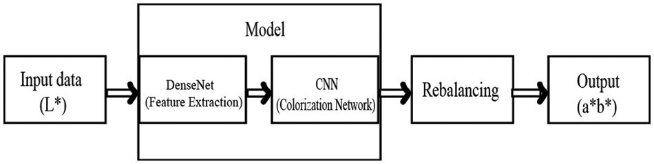
Figure 1: The organization our proposed method

3.1 Dense Network (Feature Extractor)

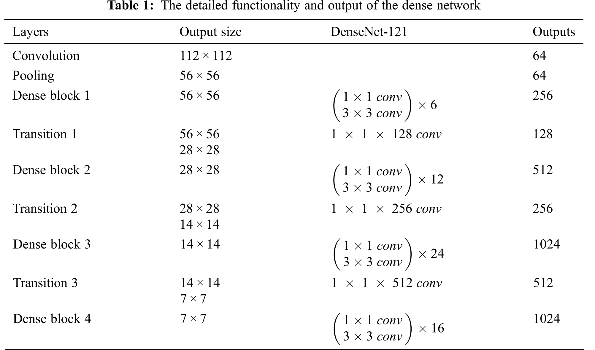
We use DenseNet as our feature extractor. Because of strong connections among its layers, DenseNet has less semantic information loss during feature extraction than other CNN architectures. DenseNet reduces the gradient vanishing problem by concatenating its output from the previous layer with all of the future layers which is shown in Fig. 2. For this it can extract high-level complex features that are very suitable for colorization. When a small color area is inside the color of a large area, the large color area affects the small color area and wants to blend its background. It is possible to retain the color in small areas by extracting high-level and complex features. That’s why we use DenseNet as our feature extractor. We modify the first convolutional layer of DenseNet to make the model suitable for lightness input. We discard the last linear layer to create a H32×W32×1024 feature representation from DenseNet. These features are used as input in the colorization network, which is a CNN. The different convolutional layers and outputs of DenseNet are shown in Table 1.

Figure 2: The architecture of dense block

3.2 CNN (Colorization Network)

The network takes H32×W32×1024 feature representation as input which is the output of DenseNet and applies a series of convolutional and up-sampling layers. For up-sampling, we use the basic nearest-neighbor technique. The network outputs are H×W×2 a * b * tensor. The different convolutional layers and their outputs are presented in Table 2.

At the time of training, our proposed model reads a batch of N images. We use Mean Square Error (MSE) as a loss function to measure the disparity between the predicted a * b * and the ground-truth a * b * value. Because the MSE is great for ensuring that our trained model has no outlier predictions with huge errors since the MSE puts larger weight on these errors due to the squaring part of the function [50]. The loss function is shown as follows:

MSE=1W×H×N∑W⁡∑H⁡∑N⁡{Y(i,j)−X(i,j)}2 (1)

where Y(i, j) and X(i, j) denotes (i, j)th pixel of the predicted and original a * b * images, respectively. Moreover, W and H represent the width and height of the sample image, and N refers to the number of images contains per batch. During training, we use Adam Optimizer to backpropagate the loss to update the learning parameters of both DenseNet and CNN [51].

3.3 Color Rebalancing

In the training dataset, the number of desaturated color pixels is much more than saturated color pixels. The desaturated color pixel is due to the backgrounds (clouds, pavement, dirt, walls, etc.). Hence, the loss function is dominated by desaturated a * b * values. To overcome this problem, we divide the entire a * b * channel into subregions according to the small intensity range of gray image. Then we apply the average filter in each subregion and then apply Gamma transformation in the entire a * b * channel to saturate the image. The proposed color rebalancing algorithm is shown step by step as follows:

Step 1: Input gray image and its predicted a * b * from the learning model.

Step 2: Split the entire input gray image region into P = MN subregions, where each subregion contains intensities [i:i+255M] . Where, i = 0, 255M , 255×2M , ……2-stage k-means clustering technique is applied to divide the region. In 1st stage, the gray image values (intensity values) are divided into M clusters, and in 2nd stage, the intensity of each M cluster is divided into N clusters based on coordinate values.

Step 3: Split the predicted a * b * channel (output of CNN model) into P subregions according to the coordinates of each subregion found in Step 2.

Step 4: Apply an average filter in each subregion of the a * b * channel to smooth the color components of subregions.

Step 5: Apply Gamma transformation to the entire a * b * channel to saturate the image. γ1 for the positively-valued pixels and γ2 for the negatively-valued pixels.

Step 6: Merge the gray (L *), modified a * b * channel and convert to RGB.

4  Experimental Results

4.1 Datasets

We use two datasets Place365 standard [52] and CelebA [53], for our experiment. The Place365-standard dataset has approximately 1.8 million RGB images for 365 scene categories, where there are at most 5000 images per category. We take about 1,000,000 images and divide them into two categories: indoor and outdoor where each category consists of approximately 500,000 images. The CelebA dataset has 202,599 RGB images of human faces. For training, we convert all RGB images to L * a * b * space. All images are resized into 224 × 224.

4.2 Runtime Environment

We have implemented our proposed model in PyTorch [54]. Adam optimizer [51] has been used to backpropagate the loss during the training. We train and validate our proposed model using the Google Colab [55] with a Graphics Processing Unit (GPU) runtime. We could maximize batch size 64 to avoid the overflow of GPU memory. Google Colab allows running programs for 12 h at a time. For this reason, we were able to perform two epochs a day. It took approximately 12 days to complete 20 epochs (147,600 iterations) for indoor images, 12 days to achieve 20 epochs (149,840 iterations) for outdoor, and six days to perform 20 epochs (60,780 iterations) for human faces during training.

For rebalancing, the CNN model’s output is used as input. The input gray values (intensity) is first divided into M cluster by k-means clustering. Then the intensity values of each cluster are divided into N clusters based on coordinate values (region). Therefore, we get MN regions in the whole image. So, k-means for M cluster with 224 × 224 (whole image) data points + M times k-means for N cluster with average 224x224M data points is the complexity of the process. M times k-means on average 224x224M data approximates 1 k-means on 224 × 224 (whole image) data points. Thus, the entire clustering can be considered 2 k-means on the whole 224 × 224 (whole image) data points on average.

4.3 Numerical Results

We train indoor and outdoor datasets keeping 20,000 images for validation. For the human dataset, we train all images keeping 8,000 images for validation. Each category has been trained separately because Colab cannot perform a single epoch taking 1.2 million images within a session of 12 h. We experimentally set the values of the parameters of the rebalancing algorithms which are shown in Table 3. For testing, images can be categorized first into indoor, outdoor and human. We categorize them manually and fit them into the network.

In Fig. 3, we have shown five different images of indoor, outdoor, and human datasets. The results look very similar to the ground truth. Our first and fifth images contain the same color but are deeper and brighter compared with the ground truth. The second and fourth images are very similar to the ground truth. The third image chooses the wrong color for certain areas but looks visually satisfactory. In Fig. 4, we have shown five different images. Here we have shown the outputs both with and without color rebalancing including gray and ground truth images. There exists object color mismatch and desaturated color in the results without rebalancing. But rebalancing the output images shows that there is no object color mismatch and desaturated or grayish color problems.

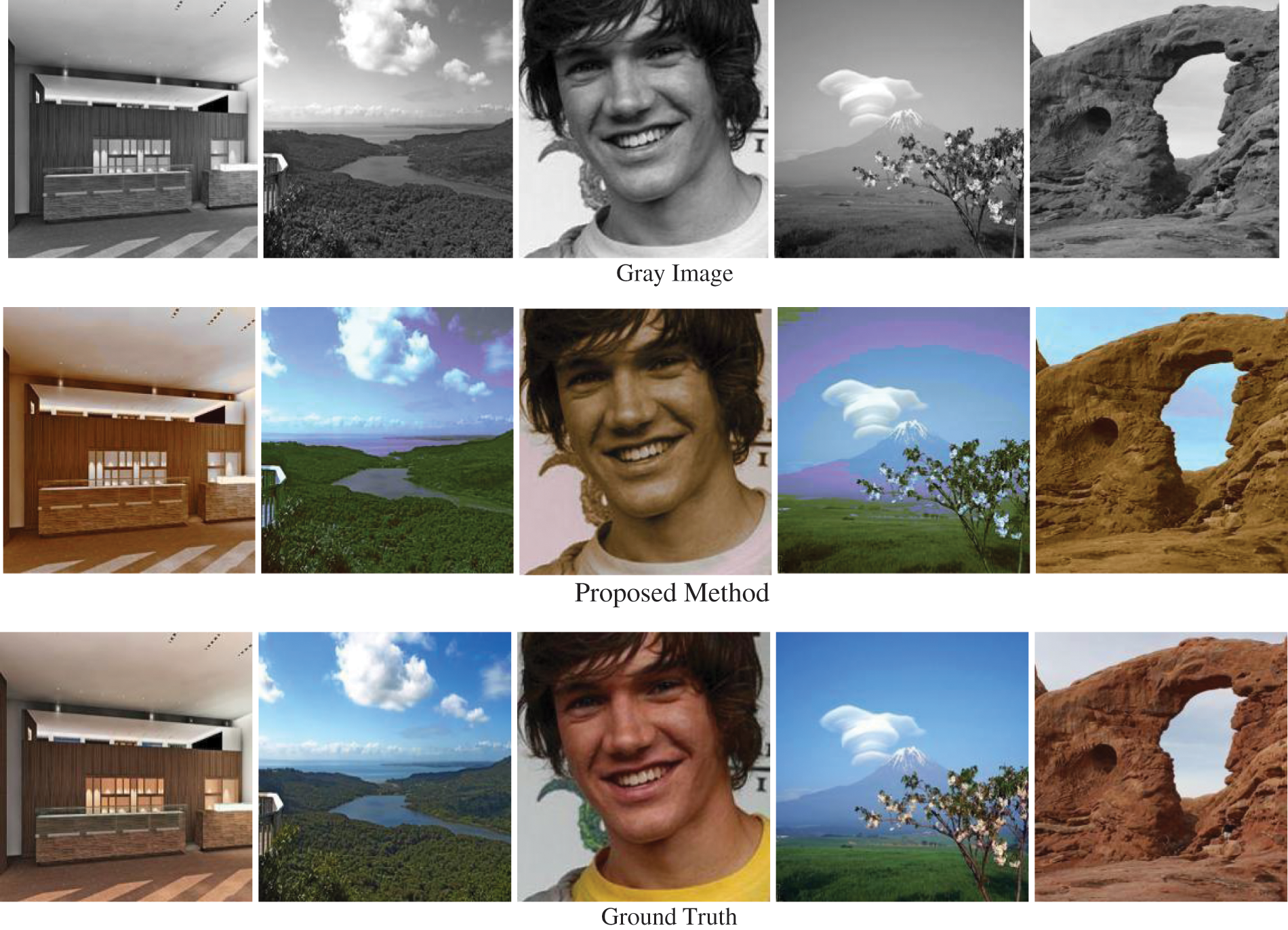
Figure 3: Colorization from our proposed model and ground truth on a diversity of scenes which includes indoor, outdoor and human. Images produced by the proposed method are very similar to ground truth images. Besides output images produced from the proposed approach are brighter than the ground truth

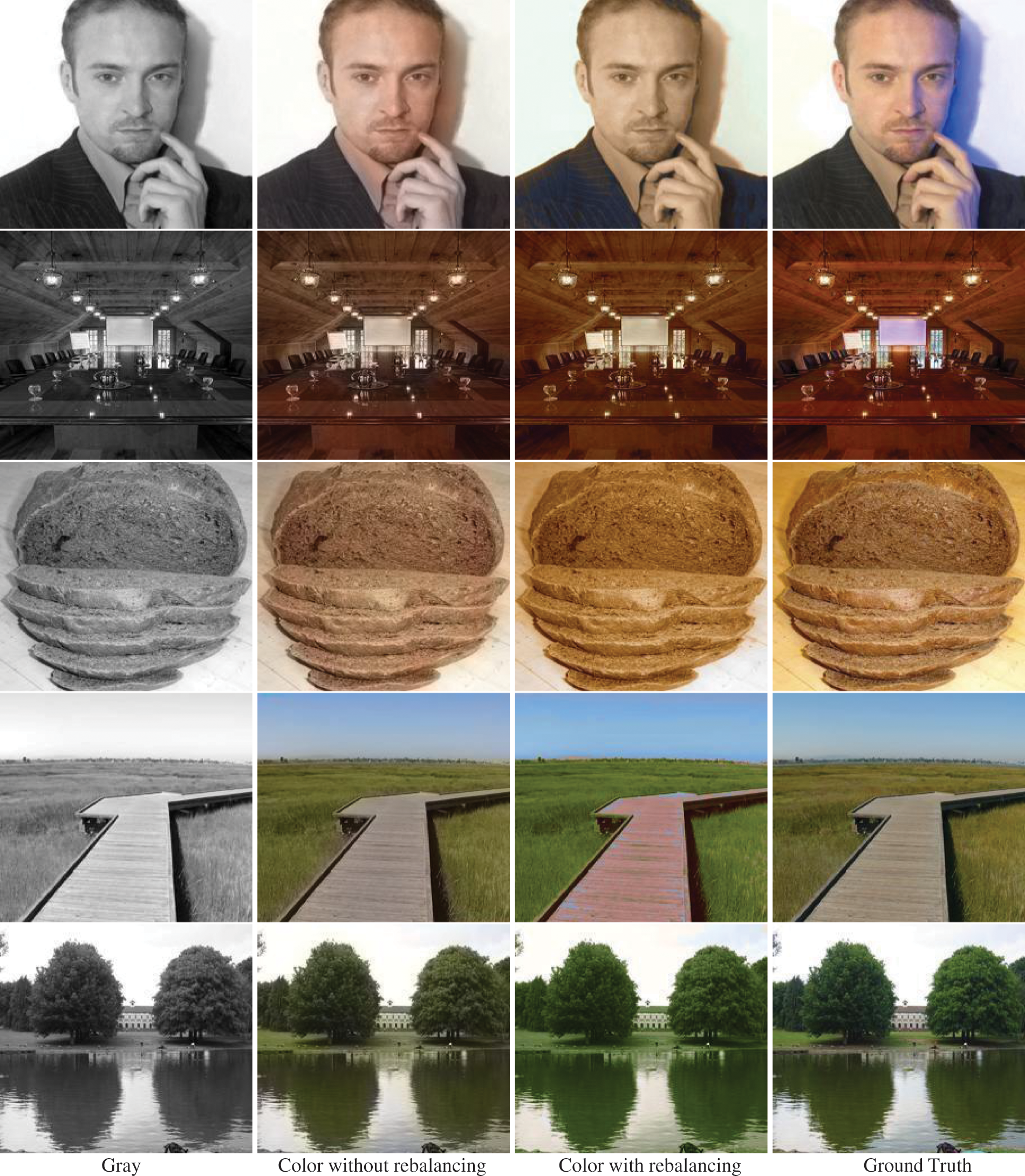
Figure 4: Results of our proposed method on five different types of images. The first column contains input gray images, the second column is the result of our proposed method without color rebalancing, the third column is the result of our proposed method with color rebalancing and the fourth column is the ground truth images. Except for the first image, every image looks very similar to the ground truth. The result of the first image after color rebalancing does not contain a shadow blue color as in the ground truth image. However, it looks very plausible to visualize

We have compared our results with different methods (Deoldify [56], Iizuka et al. [5], Larsson et al. [17], Zhang et al. [25]). We have taken six images randomly from the dataset and the corresponding outputs are shown in Fig. 5 along with the ground truth. From Fig. 5, we see that Deoldify [56] choose a desaturated color in every image except 3rd. Iizuka [5] color well in images 4, 5 & 6 but form desaturation and color mismatch in images 1, 2 & 3. Larsson [17] & Su [9] over colorize images 1 & 6 and form desaturation in in images 2, 3, 4 & 5. Zhang [25] forms saturation but over colorize images 1, 2, 3 & 6. We find that there is no significant difference visually between the image generated from the proposed approach and the ground truth.

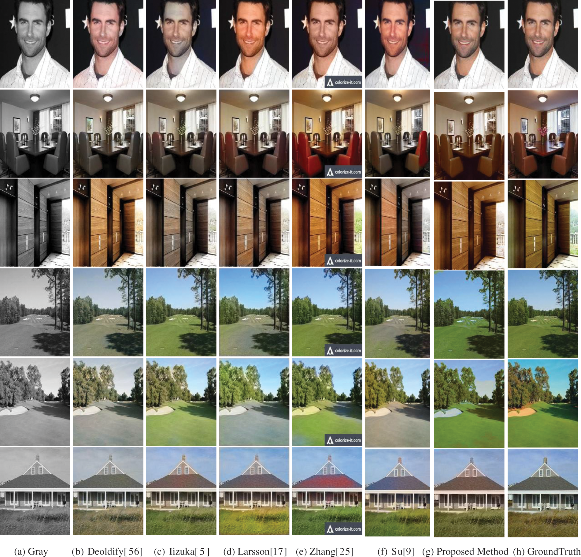
Figure 5: Comparison of results of our proposed method with some other methods and ground truth image

We use Peak Signal-to-Noise Ratio (PSNR) and Structural Similarity Index Measure (SSIM) [57] to compare the quantitative performance among different methods. PSNR can roughly assess the image quality, and usually, the higher PSNR, the better.

It measures the similarity between the reconstruction image and ground truth from the pixel level. SSIM estimates the correlation between two images (generated and ground truth), and higher SSIM signifies more structural similarity. PSNR can be defined as follows:

PSNR=10log102552MSE (2)

where, MSE=1W×H×N∑W⁡∑H⁡∑N⁡{Y(i,j)−X(i,j)}2

Here, Y(i, j) and X(i, j) denote (i, j) th pixels in both the output and ground truth RGB images. Moreover, W and H represent the width and height of the sample. Besides, SSIM can be defined as follows:

SSIM(X,Y)=(2μXμY+c1)(2σXY+c2)(μX2+μY2+c1)(μX2+μY2+c2) (3)

where, μX and μY present the average of X and Y respectively whereas σX and σY indicate the variance of X and Y, respectively. Moreover, σXY expresses the covariance of X and Y. Here, c1 = (k1L)2 and c2 = (k2L)2 with k1 = 0.01, k2 = 0.03, and L = 255 [58].

Table 4 shows a comparison of PSNR values among different methods for different images of three classes. We find from Table 4 that the PSNR values for the proposed method are better than that of all other comparing approaches for all the considered images except in the case of the second image for Larsson [17]. On average, the PSNR value of the proposed approach is 20.32%, 10.17%, 18.28%, and 32.01% better than Deoldify [56], Iizuka [5], Larsson [17], and Zhang [25], respectively.

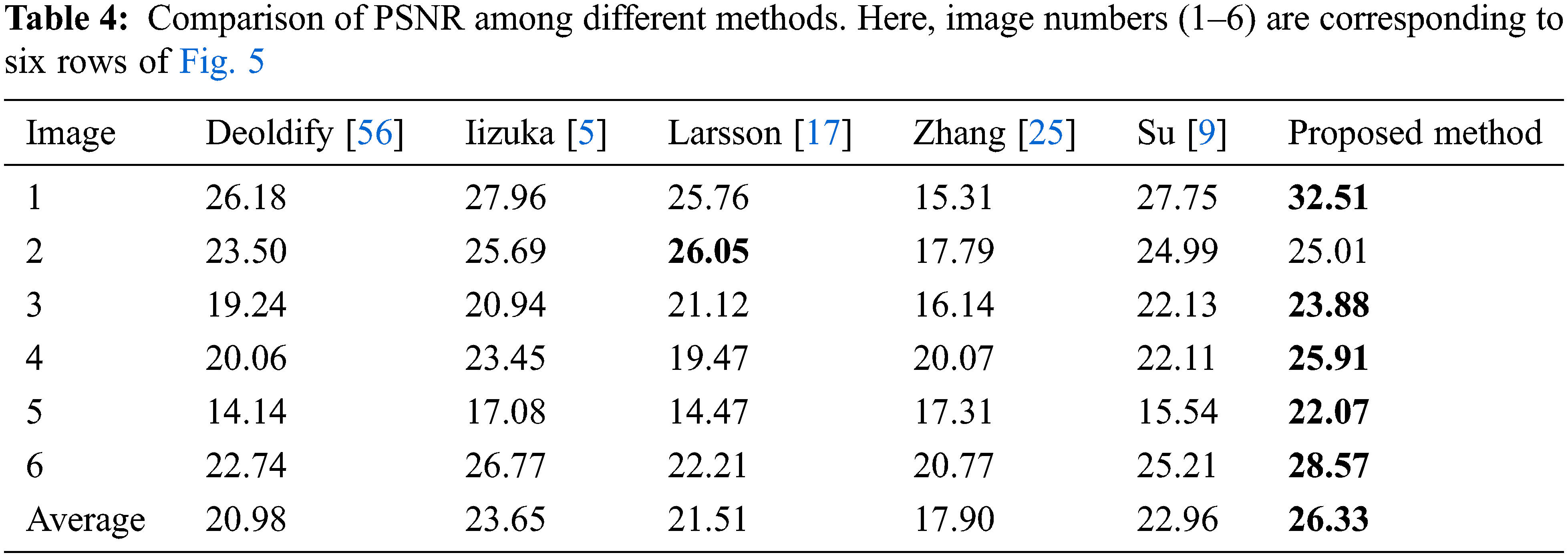
Fig. 6 shows a comparison of SSIM values for different images among comparing methods. We find from Fig. 6 that the SSIM values of the proposed approach are very much comparable with other methods in most of the cases. On the average, this value of the proposed method is 12.70%, 1.38%, 7.58%, 9.05% and 8.19% higher than Deoldify [56], Iizuka [5], Larsson [17], Zhang [25] and Su [9] respectively.

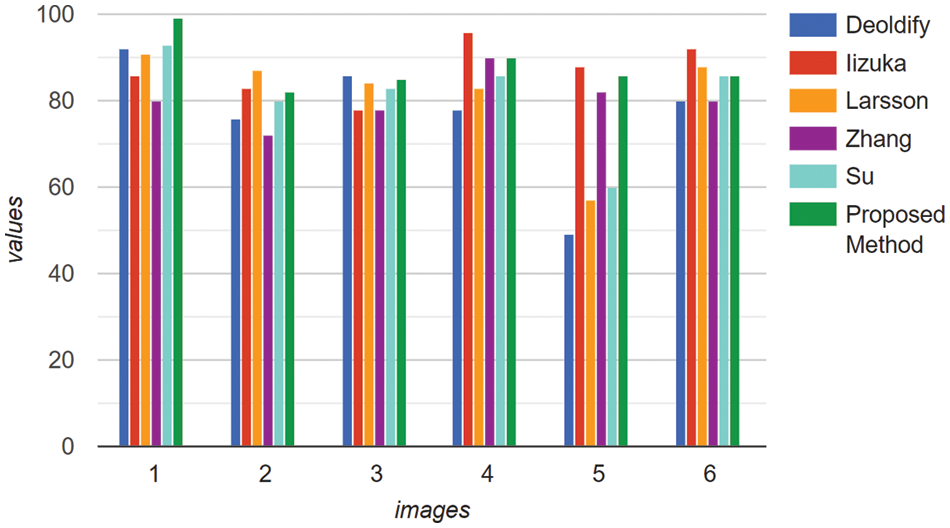
Figure 6: Comparison of SSIM value of the proposed method with other methods with respect to ground truth. Here, the image numbers are corresponding to that of Table 4

For comparing the results among different methods, we also perform histogram analysis of constructed images with ground truth images, and this is depicted in Fig. 7. From the comparison, we see that, for image #1, every method shows the same data distribution without any major interruption. For image #2, Deoldify and the proposed method show satisfactory distribution whereas Iizuka, Zhang, Larsson and Su show noticeable interruption. For image #3, the proposed method shows only satisfactory distribution whereas Iizuka and Zhang show moderate interruption, and Deoldify, Larsson and Su show acute interruption.

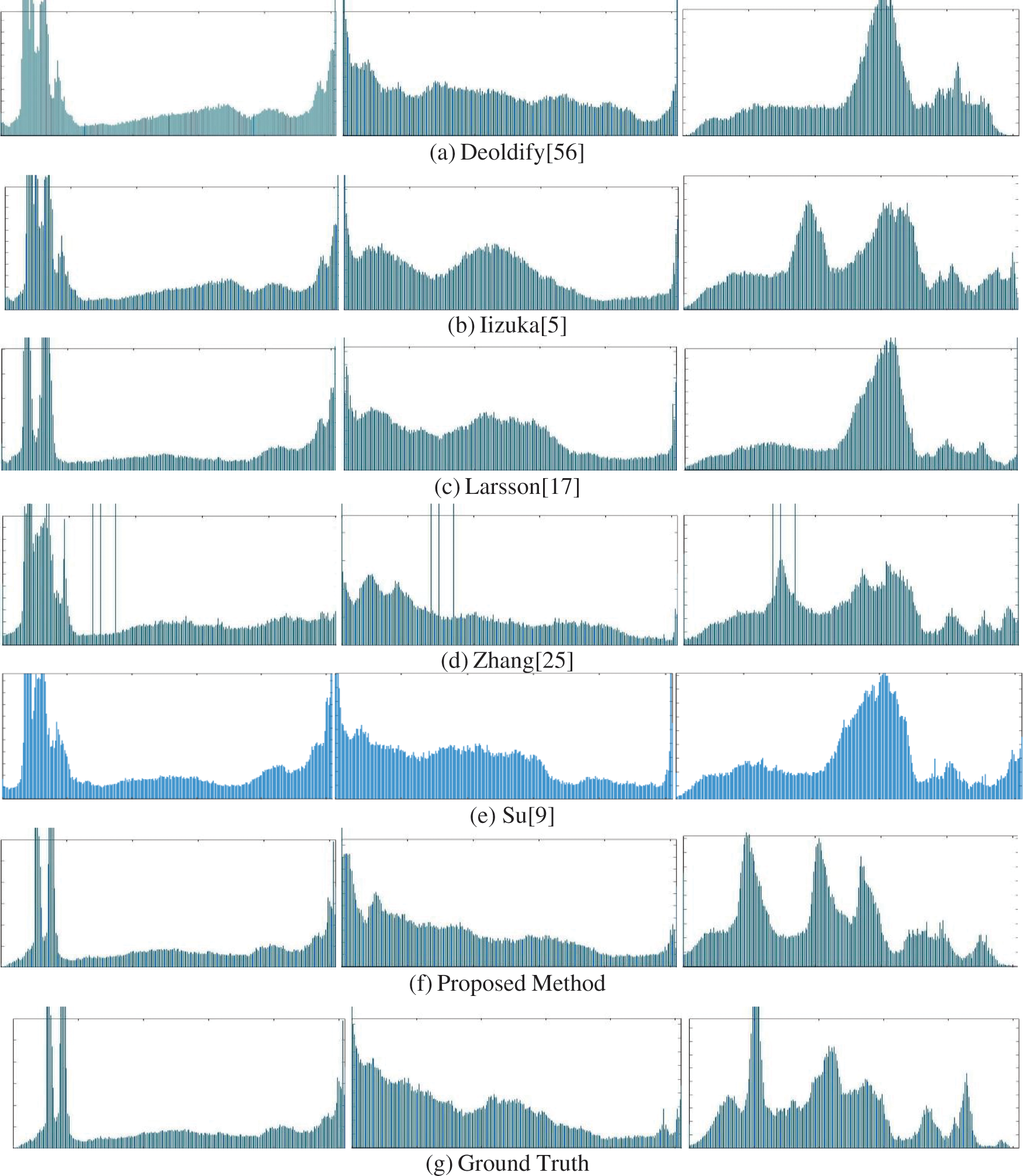
Figure 7: Comparison of the histogram of the proposed method with other methods and ground truth. Here, columns 1, 2, and 3 represent histograms of image #1, image #3, and image #5, respectively

There are no significant differences in histograms of the produced illustrations for the proposed method and the corresponding ground truth, and they match better than with any of the comparing methods’ histograms.

We have also tested our proposed model with two historical images (Figs. 8a and 8b) and the results are shown in Figs. 8c and 8d, respectively. There is no ground truth color of these images for comparison. Human perception is the only way to judge these results.

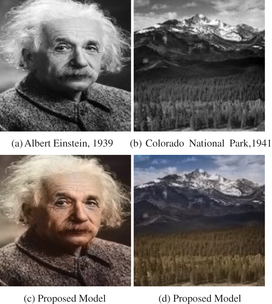
Figure 8: Historical images and their colorized results of the proposed method with color rebalancing

4.4 Results Analysis and Discussions

Colorization is a very ill-posed problem as there is no linear formula to generate color values from luminance components. Deep learning techniques shows notable progress in colorization process in recent times. In this paper, we proposed a new encoder-decoder model for image colorization. We used a dense neural network for feature extraction as the encoder and CNN for color component prediction as the decoder. The performance of the deep learning model largely depends on the balance state of the dataset. Unlike other image processing problems, in colorization task, balance data indicate the balance state at the feature (intensity) level instead of the sample level. When a small color area is inside color of a large area, the larger color area affects the small color area and wants to blend its background. It is possible to retain the color in small areas by extracting fine and complex features. DenseNet can extract high-level complex features (Feature in all possible patterns so that minor pixel values can also be traced). For this purpose, we used DenseNet as a feature extractor for our proposed method. The number of desaturated pixels is higher than the number of saturated pixels in an image because the background areas are very large than the main object area. For this reason, color bleeding problems and desaturated problems are found in the predicted color image. To solve the problems, we proposed a color rebalancing method, where we separate different color regions using 2 stage k-means clustering techniques. Then we apply the average filter region-wise to solve color bleeding problem and gamma transformation to solve desaturation. We found our proposed method solved the abovementioned problem effectively which is shown in Fig. 4. We compared our proposed method with several works and found the visuals of our proposed method outperform other methods, which is shown in Fig. 5. Utilizing the PSNR, SSIM, and Histogram assessment measures, we also compared our suggested strategy with other methodologies. We found our proposed method performs well compared to other methods which are shown in Table 4, Figs. 6 and 7. We also tested our proposed model using historical images and got plausible color visuals which are shown in Fig. 8.

A feature-balanced dataset can be created by capturing images that contain every possible color in an equal proportional ratio for tackling the imbalance data problem to improve the model performance. Because the deep learning method performs depending on the balance state of training data. Besides, the performance of the rebalancing method depends on the performance of the deep learning model. Because rebalancing strategies are used at the conclusion of the learning process in the way we’ve proposed the method. The anticipated a * b * might be more vivid if it can be applied to the learning process.

5  Conclusion and Future Work

In this paper, we present a new image colorization approach applying an improved encoder-decoder CNN model. We apply DenseNet for deep feature extraction from input gray image and a CNN for predicting a * b * channel. We then rebalance the a * b * channel by applying the average filtering technique. Then we apply Gamma transformation to enhance the image quality. We evaluate our proposed method on a wide variety of images from indoor, outdoor and human faces. Our proposed method gives impressive results having bright color in every region. Our proposed method also solves object color mismatch problems and grayish color problems.

In our proposed method, rebalancing techniques are applied at the end of the learning process. If it can be applied to the a * b * estimated by the proposed model in each epoch before the loss calculation, the predicted a * b * may be more vibrant. So, in the future, we will incorporate rebalancing techniques in the learning process. Future works will also focus on prioritizing rarely appeared color pixels during training for increasing their impact.

Acknowledgement: This Research is supported by Khulna University Research Grant (Project ID: 23/2019). We would like to give special thanks to Taif University Research supporting Project Number (TURSP-2020/10), Taif University, Taif, Saudi Arabia.

Funding Statement: Taif University Researchers Supporting Project Number (TURSP-2020/10), Taif University, Taif, Saudi Arabia.

Conflicts of Interest: The authors declare that they have no conflicts of interest to report regarding the present study.

References

1. Y. C. Huang, Y. S. Tung, J. C. Chen, S. W. Wang and J. L. Wu, “An adaptive edge detection based colorization algorithm and its applications,” in Proc. 13th Annual ACM Int. Conf. on Multimedia, Hilton, Singapore, pp. 351–354, 2005. [Google Scholar]
2. A. Levin, D. Lischinski and Y. Weiss, “Colorization using optimization,” in Proc. ACM SIGGRAPH 2004 Papers, Los Angeles, California, USA, pp. 689–694, 2004. [Google Scholar]
3. L. Yatziv and G. Sapiro, “Fast image and video colorization using chrominance blending,” IEEE Transactions on Image Processing, vol. 15, no. 5, pp. 1120–1129, 2006. [Google Scholar]
4. J. An, K. K. Gagnon, Q. Shi, H. Xie and R. Cao, “Image colorization with convolutional neural networks,” in Proc. 12th Int. Congress on Image and Signal Processing, BioMedical Engineering and Informatics (CISP-BMEI), Suzhou, China, pp. 1–4, 2019. [Google Scholar]
5. S. Iizuka, E. Simo-Serra and H. Ishikawa, “Let there be color! joint end-to-end learning of global and local image priors for automatic image colorization with simultaneous classification,” ACM Transactions on Graphics (ToG), vol. 35, no. 4, pp. 1–11, 2016. [Google Scholar]
6. A. Sousa, R. Kabirzadeh and P. Blaes, “Automatic colorization of grayscale images,” Department of Electrical Engineering, Stanford University, 2013. http://cs229.stanford.edu/proj2013/KabirzadehSousaBlaes-AutomaticColorizationOfGrayscaleImages.pdf [Google Scholar]
7. T. Welsh, M. Ashikhmin and K. Mueller, “Transferring color to greyscale images,” in Proc. 29th Annual Conf. on Computer Graphics and Interactive Techniques, Texas, San Antonio, USA, pp. 277–280, 2002. [Google Scholar]
8. R. K. Gupta, A. Y. S. Chia, D. Rajan, E. S. Ng and H. Zhiyong, “Image colorization using similar images,” in Proc. 20th ACM Int. Conf. on Multimedia, Nara, Japan, pp. 369–378, 2012. [Google Scholar]
9. J. W. Su, H. K. Chu and J. B. Huang, “Instance-aware image colorization,” in Proc. IEEE/CVF Conf. on Computer Vision and Pattern Recognition, Seattle, WA, USA, pp. 7968–7977, 2020. [Google Scholar]
10. V. S. Devi and S. Kannimuthu, “Author profiling in code-mixed WhatsApp messages using stacked convolution networks and contextualized embedding based text augmentation,” Neural Processing Letters, pp. 1–26, 2022. http://dx.doi.org/10.1007/s11063-022-10898-3 [Google Scholar]
11. K. C. Raja and S. Kannimuthu, “Conditional generative adversarial network approach for autism prediction,” Computer Systems Science and Engineering, vol. 44, no. 1, pp. 741–755, 2023. [Google Scholar]
12. S. Albawi, T. A. Mohammed and S. Al-Zawi, “Understanding of a convolutional neural network,” in Proc. 2017 Int. Conf. on Engineering and Technology (ICET), Antalya, Turkey, pp. 1–6, 2017. [Google Scholar]
13. J. Hwang and Y. Zhou, “Image colorization with deep convolutional neural networks,” in Stanford University, Tech. Rep., vol. 219, Stanford, CA 94305, United States, pp. 1–7, 2016. [Google Scholar]
14. F. Baldassarre, D. G. Mor ́ın and L. Rod ́es-Guirao, “Deep koalarization: Image colorization using CNNs and inception-ResNet-v2,” arXiv peprint arXiv:1712.03400, 2017. [Google Scholar]
15. P. Qin, Z. Cheng, Y. Cui, J. Zhang and Q. Miao, “Research on image colorization algorithm based on residual neural network,” in CCF Chinese Conf. on Computer Vision, Singapore, Springer, pp. 608–621, 2017. [Google Scholar]
16. R. Dahl, “Automatic colorization,” 2016. [Online]. Available: https://tinyclouds.org/colorize. [Google Scholar]
17. G. Larsson, M. Maire and G. Shakhnarovich, “Learning representations for automatic colorization,” in European Conf. on Computer Vision (ECCV), Cham, Springer, pp. 577–593, 2016. [Google Scholar]
18. J. Dai, B. Jiang, C. Yang, L. Sun and B. Zhang, “Local pyramid attention and spatial semantic modulation for automatic image colorization,” in CCF Conf. on Big Data, Singapore, Springer, pp. 165–181, 2022. [Google Scholar]
19. V. Singh, A. Deepak and P. Sharma, “Image colorization using deep convolution autoencoder,” in Proc. of Int. Conf. on Recent Trends in Computing, Singapore, Springer, pp. 431–441, 2022. [Google Scholar]
20. D. Wu, J. Gan, J. Zhou, J. Wang and W. Gao, “Fine-grained semantic ethnic costume high-resolution image colorization with conditional GAN,” International Journal of Intelligent Systems, vol. 37, no. 5, pp. 2952–2968. 2022. [Google Scholar]
21. H. Guo, Z. Guo, Z. Pan and X. Liu, “Bilateral Res-unet for image colorization with limited data via GANs,” in Proc. 2021 IEEE 33rd Int. Conf. on Tools with Artificial Intelligence (ICTAI), Washington, DC, USA, pp. 729–735, 2021. [Google Scholar]
22. M. Xu and Y. Ding, “Fully automatic image colorization based on semantic segmentation technology,” PLOS ONE, vol. 16, no. 11, pp. 1–25, 2021. [Google Scholar]
23. M. Hesham, H. Khaled and H. Faheem, “Image colorization using scaled-YOLOv4 detector,” International Journal of Intelligent Computing and Information Sciences, vol. 21, no. 3, pp. 107–118, 2021. [Google Scholar]
24. N. Zhang, P. Qin, J. Zeng and Y. Song, “Image colorization algorithm based on dense neural network,” International Journal of Performability Engineering, vol. 15, no. 1, pp. 270–280, 2019. [Google Scholar]
25. R. Zhang, P. Isola and A. A. Efros, “Colorful image colorization,” in European Conf. on Computer Vision, Singapore, Springer, pp. 649–666, 2016. [Google Scholar]
26. G. Huang, Z. Liu, L. V. D. Maaten and K. Q. Weinberger, “Densely connected convolutional networks,” in Proc. IEEE Conf. on Computer Vision and Pattern Recognition (CVPR), Honolulu, Hawaii, USA, pp. 4700–4708, 2017. [Google Scholar]
27. C. Szegedy, S. Ioffe, V. Vanhoucke and A. A. Alemi, “Inception-v4, inception-resnet and the impact of residual connections on learning,” in Thirty-first AAAI Conf. on Artificial Intelligence, San Francisco, California, USA, AAAI Press, 2017. [Google Scholar]
28. B. Li, Y. -K. Lai, M. John and P. L. Rosin, “Automatic example-based image colorization using location-aware cross-scale matching,” IEEE Transactions on Image Processing, vol. 28, no. 9, pp. 4606–4619, 2019. [Google Scholar]
29. J. Lee, E. Kim, Y. Lee, D. Kim, J. Chang et al., “Reference-based sketch image colorization using augmented-self reference and dense semantic correspondence,” in Proc. IEEE/CVF Conf. on Computer Vision and Pattern Recognition, Seattle, WA, USA, pp. 5801–5810, 2020. [Google Scholar]
30. K. Simonyan and A. Zisserman, “Very deep convolutional networks for large-scale image recognition,” arXiv preprint arXiv:1409.1556, 2014. [Google Scholar]
31. B. Hariharan, P. Arbeláez, R. Girshick and J. Malik, “Hypercolumns for object segmentation and fine-grained localization,” in Proc. IEEE Conf. on Computer Vision and Pattern Recognition (CVPR), Boston, USA, pp. 447–456, 2015. [Google Scholar]
32. K. He, X. Zhang, S. Ren and J. Sun, “Deep residual learning for image recognition,” in Proc. IEEE Conf. on Computer Vision and Pattern Recognition (CVPR), Las Vegas, Nevada, USA, pp. 770–778, 2016. [Google Scholar]
33. L. Liu, Q. Jiang, X. Jin, J. Feng, R. Wang et al., “CASR-Net: A color-aware super-resolution network for panchromatic image,” Engineering Applications of Artificial Intelligence, vol. 114, pp. 105084, 2022. [Google Scholar]
34. A. Kumar, D. S. George and L. S. Binu, “Colorization of grayscale images using convolutional neural network and siamese network,” in Machine Intelligence and Smart Systems, Singapore, Springer, pp. 297–308, 2022. [Google Scholar]
35. G. Ozbulak, “Image colorization by capsule networks,” in Proc. IEEE/CVF Conf. on Computer Vision and Pattern Recognition Workshops, Long Beach, CA, USA, pp. 0–0, 2019. [Google Scholar]
36. G. Kong, H. Tian, X. Duan and H. Long, “Adversarial edge-aware image colorization with semantic segmentation,” IEEE Access, vol. 9, pp. 28194–28203, 2021. [Google Scholar]
37. Y. Wu, X. Wang, Y. Li, H. Zhang, X. Zhao et al., “Towards vivid and diverse image colorization with generative color prior,” in Proc. IEEE/CVF Int. Conf. on Computer Vision, Montreal, Canada, pp. 14377–14386, 2021. [Google Scholar]
38. T. -T. Nguyen-Quynh, S. -H. Kim and N. -T. Do, “Image colorization using the global scene-context style and pixel-wise semantic segmentation,” IEEE Access, vol. 8, pp. 214098–214114, 2020. [Google Scholar]
39. H. Bahng, S. Yoo, W. Cho, D. K. Park, Z. Wu et al., “Coloring with words: Guiding image colorization through text-based palette generation,” in Proc. European Conf. on Computer Vision (ECCV), Munich, Germany, pp. 431–447, 2018. [Google Scholar]
40. Y. Liang, D. Lee, Y. Li and B. -S. Shin, “Unpaired medical image colorization using generative adversarial network,” Multimedia Tools and Applications, vol. 81, no. 19, pp. 26669–26683, 2022. [Google Scholar]
41. I. Žeger, S. Grgic, J. Vuković and G. Šišul, “Grayscale image colorization methods: Overview and evaluation,” IEEE Access, vol. 9, pp. 113326–113346, 2021. [Google Scholar]
42. S. Treneska, E. Zdravevski, I. M. Pires, P. Lameski, and S. Gievska, “GAN-Based image colorization for self-supervised visual feature learning,” Sensors, vol. 22, no. 4, pp. 1599, 2022. [Google Scholar]
43. M. Wu, X. Jin, Q. Jiang, S. -J. Lee, W. Liang et al., “Remote sensing image colorization using symmetrical multi-scale DCGAN in YUV color space,” The Visual Computer, vol. 37, no. 7, pp. 1707–1729, 2021. [Google Scholar]
44. M. Sugawara, K. Uruma, S. Hangai and T. Hamamoto, “Local and global graph approaches to image colorization,” IEEE Signal Processing Letters, vol. 27, pp. 765–769, 2020. [Google Scholar]
45. M. Afifi, M. A. Brubaker and M. S. Brown, “Histogan: Controlling colors of GAN-generated and real images via color histograms,” in Proc. IEEE/CVF Conf. on Computer Vision and Pattern Recognition, Nashville, TN, USA, pp. 7941–7950, 2021. [Google Scholar]
46. T. Karras, S. Laine, M. Aittala, J. Hellsten, J. Lehtinen et al., “Analyzing and improving the image quality of StyleGAN,” in Proc. IEEE/CVF Conf. on Computer Vision and Pattern Recognition, Seattle, WA, USA, pp. 8110–8119, 2020. [Google Scholar]
47. A. R. Robertson, “The CIE 1976 color-difference formulae,” Color Research & Application, vol. 2, no. 1, pp. 7–11, 1977. [Google Scholar]
48. I. Goodfellow, Y. Bengio and A. Courville, “Deep Learning,” Cambridge, MA, USA: MIT Press, 2016. Available: http://www.deeplearningbook.org. [Google Scholar]
49. M. D. Zeiler and R. Fergus, “Visualizing and understanding convolutional networks,” in European Conf. on Computer Vision, Cham, Springer, pp. 818–833, 2014. [Google Scholar]
50. Z. Wang and A. C. Bovik, “Mean squared error: Love it or leave it? A new look at signal fidelity measures,” IEEE Signal Processing Magazine, vol. 26, no. 1, pp. 98–117, 2009. [Google Scholar]
51. D. P. Kingma and J. Ba, “Adam: A method for stochastic optimization,” arXiv preprint arXiv:1412.6980, 2015. [Google Scholar]
52. B. Zhou, A. Lapedriza, A. Khosla, A. Oliva and A. Torralba, “Places: A 10 million image database for scene recognition,” IEEE Transactions on Pattern Analysis and Machine Intelligence, vol. 40, no. 6, pp. 1452–1464, 2018. [Google Scholar]
53. Z. Liu, P. Luo, X. Wang and X. Tang, “Deep learning face attributes in the wild,” in Proc. IEEE Int. Conf. on Computer Vision(ICCV 2015), Santiago, Chile, pp. 3730–3738, 2015. [Google Scholar]
54. A. Paszke, S. Gross, F. Massa, A. Lerer, J. Bradbury et al., “Pytorch: An imperative style, high-performance deep learning library,” Advances in Neural Information Processing Systems, vol. 32, pp. 8024–8035, 2019. [Google Scholar]
55. E. Bisong, “Building machine learning and deep learning models on google cloud platform,” in Berkeley, CA: Apress, Berlin, Germany, Springer, pp. 59–64, 2019. [Google Scholar]
56. J. Antic, “A deep learning based project for colorizing and restoring old images (and video!),” 2018. [Online]. Available: https://github.com/jantic/DeOldify. [Google Scholar]
57. A. Hore´ and D. Ziou, “Image quality metrics: PSNR vs. SSIM,” in Proc. 2010 20th Int. Conf. on Pattern Recognition, Istanbul, Turkey, pp. 2366–2369, 2010. [Google Scholar]
58. Z. Wang, A. C. Bovik, H. R. Sheikh and E. P. Simoncelli, “Image quality assessment: From error visibility to structural similarity,” IEEE Transactions on Image Processing, vol. 13, no. 4, pp. 600–612, 2004. [Google Scholar]
Cite This Article
Copyright © 2023 The Author(s). Published by Tech Science Press.
This work is licensed under a Creative Commons Attribution 4.0 International License , which permits unrestricted use, distribution, and reproduction in any medium, provided the original work is properly cited.
Downloads
Citation Tools