Feature Matching Combining Variable Velocity Model with Reverse Optical Flow

1  Introduction

In recent years, with the performance improvement of edge computing platforms and the continuous emergence of excellent algorithms, autonomous localization and navigation for mobile robots, such as autonomous vehicles and drones, have been developed rapidly. The SLAM technology [1,2], which is the basis of autonomous navigation for mobile robots and 3D medical technology [3,4], has attracted more and more attention.

The visual SLAM based on the camera mainly can be divided into the optical flow method [5,6], direct method [7], and feature point method [8] according to the extraction method of image information. The feature point method is an important direction in the community of visual SLAM, which mainly extracts representative key feature points in every frame image, and then matches the feature points of two frames of images to calculate the relative pose between the two frames of images. The method has high accuracy and good robustness. When the camera moves too fastly or the tracking fails, the method can still calculate the current pose of the camera according to the matching result of feature points, i.e., repositioning [9].

The ORB-SLAM2 proposed by Mur-Artal et al. [10] is the most classic visual SLAM system based on the feature point method, with high accuracy and strong robustness. To improve the accuracy of the system, an initial pose for the current frame is first obtained in its tracking thread using a constant velocity model, then the map points mapped from the previous frame are projected onto the current frame using the initial pose transformation relationship obtained by the constant velocity model, and finally, the best matching feature points are found in a circular area centered on the projected coordinates. This method can obtain an initial pose and reduce the time consumed by the feature matching. However, it assumes that the object is moving at a constant velocity, in real scenarios, due to camera shake or fast movement, the object is mostly moving at a variable velocity, which makes the constant velocity model disabled, resulting in a failed feature points matching in a circular area centered on the projection coordinates or wrong feature point matching.

Since the matching result of feature point mathching directly affects the tracking effect and positioning accuracy of the system, it will eventually lead to a larger pose error or tracking failure. Therefore, how to effectively improve the matching accuracy is an ongoing concern for researchers. To further improve matching accuracy and reduce tracking failure of ORB-SLAM2, researchers are currently focusing on how to extract better feature points by designing better descriptors or to exploit better matching algorithm. For example, Wenle Wei [11] improved the BRIEF descriptors, Yi Cheng [12] performed fine matching using the cosine similarity, and Fu et al. [13] improved the matching accuracy by fusing point-line features. However, the improved descriptors or the used line features adversely affects the real-time performance of the feature point matching due to a higher computational complexity. In terms of improving the matching algorithm, the RANSAC (RANdom SAmple Consensus) algorithm [14] and RPOSAC (PROgressive SAmple Consensus) [15] were used to eliminate false matching. Although the above methods reduce false matching to some extent, using probabilistic random matching leads to a significant increase in computational effort and time complexity. Additionally, the probability of obtaining a plausible model by the RANSAC algorithm is related to the iteration times, i.e., computational effort increases as the iteration times increase.

To address the above challenges, this paper proposes a feature point matching algorithm combining the variable velocity model and the reverse optical flow method. In its tracking thread, a variable velocity model is proposed based on the ORB-SLAM2 framwork, which exploits the pose transformation relationship between three consecutive frames of images and combine the optical flow method to match the feature points. Firstly, calculate the initial pixel translation and take it as the initial value for the reverse optical flow method. The initial pixel translation can be obtained by the subtraction operation of the initial projection coordinates estimated by the variable velocity model and the coordinates of the feature points corresponding to the previous frame. Then, the greyscale error is minimized based on the reverse optical flow method to calculate the real-world projection coordinates by estimating the optimal pixel translation. Finally, the best matching points are found out in a circular area centered on the projection coordinates, which reduces the searching range of matching points and improves the accuracy and reliability of feature point matching, thereby estimating more accurate pose and further improving the effectiveness of tracking between two frames.

2  Methods

According to different tasks, ORB-SLAM2 is mainly divided into the tracking thread between two frames, local mapping thread, and loop closing thread. In this paper, based on its tracking thread, the proposed algorithm combines the variable velocity model and reverse optical flow method to solve the defects of traditional constant velocity models in feature point matching. The framework diagram is shown in Fig. 1.

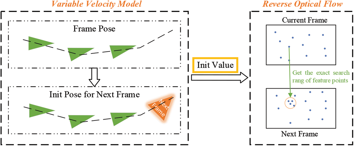
Figure 1: Framework diagram of the approach in this paper

The variable velocity model uses the pose transformation matrix between multiple frames to obtain a more accurate initial pose for the next frame. This initial pose is regarded as the initial value for the reverse optical flow. Finally, the reverse optical flow method can obtain the exact matching range of feature points and increase the matching accuracy.

2.1 Variable Velocity Model

The variable velocity model can provide a more accurate initial pose for the next frame. It assumes that the object moves with constant acceleration or deceleration in three frames, the pose transformation matrix between the first two frames is used as the base value, and the difference of the pose transformation between the first three consecutive frames is used as the updated value. By updating, the pose transformation matrix from the current frame to the next frame is derived, finally the initial pose of the next frame is derived from the derived pose transformation matrix. The flowchart of the variable velocity model is shown in Fig. 2.

1)   Calculate the pose transformation matrix between two frames

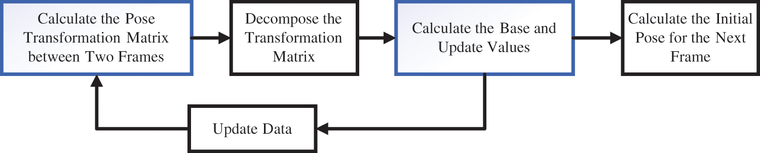
Figure 2: Flowchart of the variable velocity model

Before solving for the base and update values, we need to calculate the pose transformation matrix between the two frames, which can be obtained by transforming the reference coordinate system of the pose of the previous frame.

In this paper, Framei+1 , Framei , Framei−1 and Framei−2 represent the next frame, current frame, previous frame, and previous frame of the previous frame, respectively. In the variable velocity model, the positional transformation matrix Tcici−1 between Framei−1 and Framei is first obtained from the poses of Framei−1 and Framei , which is calculated by Eq. (1):

Tcici−1=Twci−1Twci−1 (1)

where Twci−1 and Twci represent the poses of the previous frame and the current frame, respectively.

By iterating acrosss the data, the transformation matrix Tci−1ci−2 from Framei−2 to Framei−1 can also be obtained in the same way.

2)   Calculate the base and update values

When calculating the pose transformation matrix from the current frame to the next frame, the pose transformation between the first two frames is set as the base value, and the difference of the pose transformation between the first three consecutive frames is set as the update value. , which is calculated as shown in Eq. (2):

Tci+1ci=Tcici−1⊕(Tcici−1⊖Tci−1ci−2) (2)

where Tci+1ci represents the pose transformation matrix from the current frame to the next frame, Tcici−1 is the base value, the bracketed part is the update value.

When calculating the pose transformation matrix from the current frame to the next frame, operations between pose transformation matrices are involved, such as addition or subtraction; however, the operations between the transformation matrices cannot be done directly. Therefore, there is the need to decompose the matrix into the rotation and translation parts for performing the operations. The rotation and translation parts of Tci+1ci can be expressed by Eq. (3):

{ϕci+1ci=2×ϕcici−1−ϕci−1ci−2tci+1ci=2×tcici−1−tci−1ci−2 (3)

where ϕ and t denote the euler angle of the rotation part and the translation vector of the translation part, respectively.

3)   Calculate the initial pose of the next frame

By combining the rotation part and translation part, the pose transformation matrix from the current frame to the next frame is obtained, and the initial pose Tci+1w of the next frame can be calculated by Eq. (4).

Tci+1w=Tci+1ciTciw (4)

2.2 Match Feature Points Combining Reverse Optical Flow

The reverse optical flow method can estimate the position of the feature points of the previous image on the current frame. In the combined method, a least squares problem is first constructed using the reverse optical flow method, and then the initial value for the reverse optical flow method is set by the initial pose of the current frame obtained from the variable velocity model. Finally, the Gauss_Newton iterative strategy is used to determine the feature point matching range. By finding the best feature points in the obtained matching range and minimizing the reprojection error, the exact pose of the current frame is derived, whose flowchart is shown in Fig. 3.

1)   Construction of least squares using reverse optical flow

Figure 3: Flowchart of the combining variable velocity model with reverse optical flow

In constructing the least squares, the constraint equations are first constructed based on the gray-invariant nature of the reverse optical flow, and then the equations are transformed and Taylor expanded, The steps are as follows:

a) The reverse optical flow method assumes that a pixel at (x,y) at time t moves to (x+dx,y+dy) at time t+dt with the same pixel gray value. This assumption can be expressed by Eq. (5):

I(x+dx,y+dy,t+dt)=I(x,y,t) (5)

(b) In general, the motion of pixels within a block of images is thought to be same. Assuming that there are n pixels in an image block, specially, n is set to 64 in this paper, that is, pixels in a square area with a 8×8 pixels have same motion. By performing a Taylor expansion on the left side of Eq. (5), and since the pixel gray scale of the same pixel point remains unchanged after the shift, the matrix form shown in Eq. (6) is obtained.

[[Ix,Iy]1⋮[Ix,Iy]n][uv]=−[It1⋮Itn] (6)

where u,v represents the velocity of the pixel on the x,y axis. Ix,Iy represents the gradient of the pixel on the x,y axis, and It represents the amount of variation of the pixel grayscale over time.

(c) Based on Eq. (6), the optical flow method to match feature points can be formulated as a least squares problem, which can be expressed by Eq. (7):

{minΔx,Δy⁡∑i=1n‖Ii−1(x,y)−Ii(x+Δx,y+Δy)‖22fi(Δx,Δy)=Ii−1(x,y)−Ii(x+Δx,y+Δy) (7)

2)   Calculate the initial value of reverse optical flow

The variable velocity model enables the initial value calculated by reverse optical flow method to be close to the global optimum, thus preventing the optical flow method from falling into a local minimum during optimization process. The initial value of the reverse optical flow is obtained by the difference between the coordinates before and after the projection of the feature point of the previous frame. The initial values are calculated by following steps.

a) The feature points of the previous frame are first converted into 3D map points Pmappoint in the world coordinate system, and after deriving Pmappoint , project it onto the current frame, the transformation and projection are expressed in Eq. (8):

{Pmappoint=Twci−1(K−1Zfeaturei−1Pfeaturei−1)Pfeaturei=K(TciwPmappoint)/Zfeaturei (8)

(b) Calculate the difference between Pfeaturei and Pfeaturei−1 , and set it as the initial value of the reverse optical flow. The Gauss_Newton method can be used to solve the least squares problem for the reverse optical flow, which requires to calculate Jacobi matrix. In the reverse optical flow method [16], the Jacobi matrix can be replaced with the gradient Ii−1(x,y) of the previous image frame. The Gauss_Newton equation is shown in Eq. (9):

∑i=1nJi(Δx,Δy)JiT(Δx,Δy)[ΔxΔy]=∑i=1n−Ji(Δx,Δy)fi(Δx,Δy) (9)

where Ji(Δx,Δy) represents the Jacobi matrix at fi(Δx,Δy) .

3)   Get the exact search rang

In the search for the best feature point, a Jacobi matrix Ji(Δx,Δy) is first found in a square region with 8×8 pixels, then the optimal (Δx,Δy) is solved iteratively based on the calculated Ji(Δx,Δy) and fi(Δx,Δy) .

In the process of iteration, the cost function is calculated for the correctness of the iterative result. Compare the result of the cost function after each iteration, if the result is decreasing, it means that the error is decreasing, and needs to continue iterating to update (Δx,Δy) and fi(Δx,Δy) ; otherwise, the iteration ends and the final result (Δx,Δy) is input. The cost function is expressed in Eq. (10):

Cost=∑i=1nfi(Δx,Δy)fi(Δx,Δy) (10)

By the above interation process, the more accurate position of the feature points of the previous frame image on the current frame image can be obtained, which is calculated by Eq. (11):

Pfeaturei=Pfeaturei−1+(Δx,Δy) (11)

Finally, the best feature points are matched by the feature point descriptor distance within a radius circle centered on the coordinates of Pfeaturei in the current frame.

4)   Minimize reprojection error

The reprojection error is calculated based on the initial pose Tciw obtained from the variable velocity model and the final feature point matching result, which is calculated as in Eq. (12):

Tciw∗=arg⁡minTciw12∑i=1n‖Pfeaturei−1siK(TciwPmappoint)‖22 (12)

where si represents the depth of the map point Pmappoint projected into the current frame.

The Bundle Adjustment method [17] is used to minimize the reprojection error [18] to update the initial pose forobtaining the accurate pose Tciw∗ . Finally, the variable velocity model is updated based on the accurate pose, which will prepare for the pose estimation in next frame.

3  Experiments

The experiments for the feature search and matching combining the variable velocity model and the reverse optical flow method are carried out on the platform with ubuntu18.04, where the computer is configured with an Intel Core I5-6300HQ CPU, 16G 2133 MHz RAM. The testing and analysis are conducted based on five representative sequences captured by the RGB-D camera from the public TUM dataset. In order to judge the accuracy and stability of the improved algorithm, comparative experiments with the ORB-SLAM2 system are done for each group of sequences in the dataset in terms of the Absolute Trajectory Error (ATE), Relative Pose Error (RPE) and the proportion of correctly matched feature points. To verify the effectiveness of the variable velocity model on the reverse optical flow method, comparative experiments with the traditional optical flow method without initial values were also performed in terms of the positioning accuracy.

3.1 Experimental Results and Error Analysis

The TUM dataset contains RGB and depth images, where internal parameters of camera has been calibrated and the real pose information of camera has been given, which is a standard dataset for testing the performance of visual SLAM methods.

3.1.1 Feature Matching Experiment

In the experiment, the improved method and the ORB-SLAM2 system were compared and analyzed in terms of the proportion of correct matching points between two frames during the feature matching, and the results are shown in Fig. 4. Further, the true matching results based on the D435i depth camera are shown in Fig. 5.

Figure 4: Comparison of proportion of correct matching points

Figure 5: Actual matching effect based on the D435i camera

The small green boxes in Fig. 5 represent the matched feature points. Seen from Figs. 4 and 5, the improved method can improve the proportion of correctly matched feature points on every sequence to a certain extent, with a maximum improvement of 10.2%, which indicates that the proposed method can realize more accurate feature point matching during the pose estimation between two frames. Therefore, a more accurate pose can be obtained to improve the tracking effect in the subsequent optimization process.

3.1.2 Positioning Accuracy Experiment

Tab. 1 shows the comparison results between the proposed method and the traditional ORB-SALM2 method in terms of the absolute trajectory error on five sequences of the TUM dataset. The ATE is the error between the ground truth Twcitrue and the estimated value Twciest in the SLAM system, representing the global consistency of the trajectory throughout the running phase, which is calculated by Eq. (13):

ATEall=1N∑i=1n‖log⁡(Twcitrue−1Twciest)∨‖22 (13)

Tab. 2 shows the comparison results of the RPE between the improved method and ORB-SLAM2 on five sequence of the TUM dataset. The RPE considers the relative error between Framei and Framei+1 . The smaller error means the better tracking effect between the two frames. It is calculated by Eq. (14):

RPEall=1N−1∑i=1N−1‖log⁡((Twcitrue−1Twci+1true)−1(Twciest−1Twci+1est))∨‖22 (14)

To ensure the accuracyt and reduce the variability of each run, all the test results were obtained by implementing each method five times in succession and calculating the median value of their corresponding errors.

It can be seen from Tabs. 1 and 2 that the proposed method has significantly improved the pose accuracy in every sequence of the TUM dataset, with a 36.2% improvement in the sequence fr2_desk, compared to ORB-SLAM2. Further comparison and analysis show that the error of the pose estimation of the proposed method can be reduced to a certain extent due to the accurate initial pixel translation predicted by the variable velocity model, in comparison with the single optical flow method.

To intuitively analyze the error between the improved method and ORB-SLAM2, the real trajectory and the estimated trajectory of the sequence fr1_room are shown in Fig. 6, along with the distribution of the absolute trajectory error of the two methods on the entire trajectory. At the same time, the comparison chart of the translation data and the angle data in the XYZ direction over time is shown in Fig. 7.

Figure 6: Trajectory graph and distribution of absolute trajectory error

Figure 7: Comparison of xyz axis translation data and angle data

The trajectory distribution is shown in Fig. 6, where the gradient color band from blue to red represents the magnitude size of the error of ATE, and the maximum and minimum values of the error are on the top and bottom of the color band, respectively. Seen from Figs. 6 and 7, the trajectory error of the proposed method is smaller and the trajectory is closer to the true trajectory.

It can be seen from Fig. 7 that the accuracy of the proposed method has been greatly improved in comparison with ORB-SLAM2, especially for the data on the z-axis and the pitch angle.

To further analyze the positioning accuracy of the proposed method, Fig. 8 shows the absolute pose error (APE) of the two algorithms in the sequence, where the mean, median, root mean square error (RMSE), and standard deviation (STD) are presented in detail.

Figure 8: Comparison of absolute pose error

By analyzing the absolute pose error shown in Fig. 8, the median, mean, STD, and RMSE of the absolute trajectory error of the proposed method decrease with different degrees. The tracking error between two frames decreases significantly, and the maximum error of the ORB-SLAM2 is reduced to 0.108470 m from 0.140345 m. The above experimental results demonstrate that the proposed method can reduce the error of estimated pose and improve the accuracy of tracking between two frames.

4  Conclusions

Based on ORB-SLAM2, this study proposes a feature matching algorithm combining variable velocity model and inverse optical flow method. A more accurate initial pose is obtained by the variable velocity model through the pose transformation relationship between three consecutive frames, and then the initial pose displacement of the reverse optical flow method is estimated using the initial pose calculated by the variable velocity model to obtain a more accurate range of feature point matching, which improves the proportion of correct matching points between two frames and provides better robustness and higher accuracy for the SLAM system. The experimental results demonstrate the effectiveness of the proposed method.

In the follow-up work, an IMU inertial unit and a magnetometer will be introduced to further optimize the matching between two frames, which can improve the robustness and accuracy of the SLAM system. Additionally, the re-identification algorithms [19–21] and trajectory prediction algorithm [22] can be incorporated into the system to improve the recall of loopback detection, which will reduce the cumulative error of the pose, meanwhile, real-time dense reconstruction [23], pedestrian dynamic detection [24], and object detection algorithm [25] can be added to accomplish dynamic target rejection, improve localization accuracy, and accomplish more tasks.

Funding Statement: This work was supported by The National Natural Science Foundation of China under Grant No. 61304205 and NO. 61502240, The Natural Science Foundation of Jiangsu Province under Grant No. BK20191401 and No. BK20201136, Postgraduate Research & Practice Innovation Program of Jiangsu Province under Grant No. SJCX21_0364 and No. SJCX21_0363.

Conflicts of Interest: The authors declare that they have no conflicts of interest to report regarding the present study.

References

1. H. M. Liu, G. F. Zhang and H. J. Bao, “Overview of simultaneous localization and map construction methods based on monocular vision,” Journal of Computer Aided Design and Graphics, vol. 28, no. 6, pp. 855–868, 2016. [Google Scholar]
2. A. J. Davison, I. D. Reid, N. D. Molton and O. Stasse, “MonoSLAM: Real-time single camera SLAM,” IEEE Transactions on Pattern Analysis and Machine Intelligence, vol. 29, no. 6, pp. 1052–1067, 2007. [Google Scholar]
3. X. R. Zhang, W. F. Zhang, W. Sun, X. M. Sun and S. K. Jha, “A robust 3D medical watermarking based on wavelet transform for data protection,” Computer Systems Science & Engineering, vol. 41, no. 3, pp. 1043–1056, 2022. [Google Scholar]
4. X. R. Zhang, H. L. Wu, W. Sun, A. G. Song and S. K. Jha, “A fast and accurate vascular tissue simulation model based on point primitive method,” Intelligent Automation & Soft Computing, vol. 27, no. 3, pp. 873–889, 2021. [Google Scholar]
5. H. Zhang, L. Xiao and G. Xu, “A novel tracking method based on improved FAST corner detection and pyramid LK optical flow,” in Proc. CCDC, Hefei, AH, China, pp. 1871–1876, 2020. [Google Scholar]
6. J. Hu, L. Li, Y. Fu, M. Zou, J. Zhou et al., “Optical flow with learning feature for deformable medical image registration,” Computers, Materials & Continua, vol. 71, no. 2, pp. 2773–2788, 2022. [Google Scholar]
7. J. Engel, T. Schps and D. Cremers, “LSD-SLAM: Large-scale direct monocular SLAM,” in Proc. ECCV, Zurich, Switzerland, pp. 834–849, 2014. [Google Scholar]
8. R. Mur-Artal, J. M. M. Montiel and J. D. Tardos, “ORB-SLAM: A versatile and accurate monocular SLAM system,” IEEE Transactions on Robotics, vol. 31, no. 5, pp. 1147–1163, 2015. [Google Scholar]
9. G. Yang, Z. Chen, Y. Li and Z. Su, “Rapid relocation method for mobile robot based on improved ORB-SLAM2 algorithm,” Remote Sensing, vol. 11, no. 2, pp. 149, 2019. [Google Scholar]
10. R. Mur-Artal and J. D. Tardos, “ORB-SLAM2: An open-source SLAM system for monocular, stereo, and RGB-D cameras,” IEEE Transactions on Robotics, vol. 33, no. 5, pp. 1255–1262, 2017. [Google Scholar]
11. W. L. Wei, L. N. Tan, L. B. Lu and R. K. Sun, “ORB-LBP feature matching algorithm based on fusion descriptor,” Electronics Optics and Control, vol. 27, no. 6, pp. 47–57, 2020. [Google Scholar]
12. Y. Cheng, W. K. Zhu and G. W. Xu, “Improved ORB matching algorithm based on cosine similarity,” Journal of Tianjin Polytechnic University, vol. 40, no. 1, pp. 60–66, 2021. [Google Scholar]
13. Y. Fu, S. Zheng, T. Bie, X. Q. Zhu and Q. M. Wang, “Visual-inertial SLAM algorithm combining point and line features,” Computer Application Research, vol. 39, no. 2, pp. 1–8, 2021. [Google Scholar]
14. Z. H. Xi, H. X. Wang and S. Q. Han, “Fast mismatch elimination algorithm and map construction based on ORB-SLAM2 system,” Computer Applications, vol. 40, no. 11, pp. 3289–3294, 2020. [Google Scholar]
15. M. Cao, L. Y. Hu and P. W. Xiong, “Research on RGB-D camera indoor visual positioning based on PROSAC algorithm and ORB-SLAM2,” Journal of Sensor Technology, vol. 32, no. 11, pp. 1706–1712, 2019. [Google Scholar]
16. S. Baker and I. Matthews, “Lucas-kanade 20 years on: A unifying framework,” International Journal of Computer Vision, vol. 56, no. 3, pp. 221–255, 2004. [Google Scholar]
17. H. Alismail, B. Browning and S. Lucey, “Photometric bundle adjustment for vision-based slam,” in Proc. ACCV, Taipei, TWN, China, pp. 324–341, 2016. [Google Scholar]
18. M. Buczko and V. Willert, “Flow-decoupled normalized reprojection error for visual odometry,” in Proc. ITSC, Rio, Brazil, pp. 1161–1167, 2016. [Google Scholar]
19. W. Sun, G. Z. Dai, X. R. Zhang, X. Z. He and X. Chen, “TBE-Net: A three-branch embedding network with part-aware ability and feature complementary learning for vehicle re-identification,” IEEE Transactions on Intelligent Transportation Systems, vol. 21, no. 3, pp. 1–13, 2021, https://doi.org/10.1109/TITS.2021.3130403. [Google Scholar]
20. X. R. Zhang, X. Chen, W. Sun and X. Z. He, “Vehicle re-identification model based on optimized denseNet121 with joint loss,” Computers, Materials & Continua, vol. 67, no. 3, pp. 3933–3948, 2021. [Google Scholar]
21. W. Sun, G. C. Zhang, X. R. Zhang and X. Zhang, “Fine-grained vehicle type classification using lightweight convolutional neural network with feature optimization and joint learning strategy,” Multimedia Tools and Applications, vol. 80, pp. 30803–30816, 2021. [Google Scholar]
22. B. Yang, G. C. Yan, P. Wang, C. Y. Chan, X. Song et al., “A novel graph-based trajectory predictor with pseudo-oracle,” IEEE Transactions on Neural Networks and Learning Systems, vol. 17, no. 4, pp. 1–15, 2021, https://doi.org/10.1109/TNNLS.2021.3084143. [Google Scholar]
23. J. Niu, Q. Hu, Y. Niu, T. Zhang and S. K. Jha, “Real-time dense reconstruction of indoor scene,” Computers, Materials & Continua, vol. 68, no. 3, pp. 3713–3724, 2021. [Google Scholar]
24. B. Yang, W. Q. Zhan, P. Wang, C. Y. Chan, Y. F. Cai et al., “Crossing or not? context-based recognition of pedestrian crossing intention in the urban environment,” IEEE Transactions on Intelligent Transportation Systems, vol. 23, no. 6, pp. 5338–5349, 2022. [Google Scholar]
25. W. Sun, L. Dai, X. R. Zhang, P. S. Chang and X. Z. He, “RSOD: Real-time small object detection algorithm in UAV-based traffic monitoring,” Applied Intelligence, vol. 52, no. 8, pp. 8448–8463, 2022. [Google Scholar]
Cite This Article
Copyright © 2023 The Author(s). Published by Tech Science Press.
This work is licensed under a Creative Commons Attribution 4.0 International License , which permits unrestricted use, distribution, and reproduction in any medium, provided the original work is properly cited.
Downloads
Citation Tools