De-Noising Brain MRI Images by Mixing Concatenation and Residual Learning (MCR)

1  Introduction

The brain magnetic resonance imaging (MRI) technique has much importance in diagnosing brain diseases such as bleeding, swelling, problems with the way the brain develops, tumors, infections, inflammation, damage from an injury or a stroke, and problems with the blood vessels [1]. However, the quality of brain MR images has often been disturbed and degraded by the salt & pepper and Gaussian noises due to the limitation of hardware technology during acquisition. For example, in Fig. 1, we can see that the quality of the original brain MR image is badly affected by the salt & pepper and Gaussian noises; therefore, the accuracy of the diagnosis process of brain diseases is also affected. Hence the de-noising process is a vital and challenging task for the correct analysis of the MR brain images for the diagnostic process.

Figure 1: The first image is the original clean brain MR image without any noise, the second MR image has been corrupted by the salt & pepper noise, and the third image is disturbed by the gaussian noise

In the last decades, four main types of different de-noising methods have been proposed to remove noises from MR images for analysis purposes. These de-noising techniques are based on (i) partial differential equations [2], (ii) domain transformation [3], (iii) non-local means techniques [3], and (iv) Convolutional Neural Networks [4].

The de-noising methods of MR images based on partial differential equations use anisotropic filters and Gaussian filters to remove noise from MR images [5], but it gives the wrong approximation of signal-to-noise ratio (SNR) images; therefore Gaussian de-noising method is replaced by the Rician de-noising method for improvement purposes [6]. The de-noising method is based on the fourth-order differential equations proposed in [7]. In image processing and computer vision, the non-linear diffusion filters are used to clean noisy images; therefore, these filters are used in [8] to clean MR images. Also, noise-driven diffusion filters denoise MR images by minimizing the mean squared error [9], and further improvements have been made in [10].

The de-noising methods based on domain transformation, the wavelet transform (WT), and discrete cosine transformation (DCT) techniques are used to clean MR images from noise. The routine wavelet packets are used to unperturbed the MR images in [11]. The filters are based on wavelet transformation to denoise MR images [12]. The wavelet filters have been boosted during the cleaning process of images by using the various threshold techniques in [13].

In non-local mean (NLM) de-noising techniques, the NLM filters are implemented in the noise removal process from brain MR images [14]. The NLM filtering methods of MR images have been used NLM filters to reduce the redundant information which causes the noise in images [15–21]. For 3-D MR images, optimized NLM filters try to denoise the images [16]. In method [19], the adaptive non-local means filters are used to de-noising MR images.

Many use deep learning algorithms, especially Convolutional Neural Networks (CNNs), for medical image de-noising, segmentation, super-resolution, and de-hazing [22–25]. A fast CNN-based de-noising method of MR images called FFD-Net is introduced in [25], trained for mapping noisy MR images into clean images. Another method based on CNN, called DMIR (de-noising MRI), has been used as an encoder-decoder structure to separate the noise and essential features of the noisy images and then reconstruct new images without perturbation [4].

The above-described de-noising methods of MR images have gained convincing success. However, they still have some gaps, such as the dependency on the cognition of experts, much prior knowledge is required to reconstruct images without noise, not applicable in the application yet, and mainly not performed well when the noise level in the images increases shown in Fig. 1.

This paper proposes a novel method to denoise brain MR images, followed by the fourth type of de-noising method based on deep learning algorithms like CNNs. In addition, we have proposed a de-noising method by mixing concatenation and residual learning (MCR) techniques to remove noise from brain MR images for further processing, such as brain disease diagnostic or classification. The remaining work is organized as follows; Section 2 consists of two state-of-the-art de-noising filters, median and Wiener filters, compared with our proposed MCR learning de-noising method for salt & pepper and Gaussian noises. Section 3 describes the salt & pepper and Gaussian noise, which often severely affect the quality of the brain MR images. Section 4 presents and explains the proposed MCR learning de-noising method. Section 5 comprises results and discussions, and Section 6 concludes the work.

The contribution of our work is summarized as follows:

•   We mix the two types of deep learning techniques such as concatenation and residual learning to develop a robust de-noising method to clean brain MR images from salt & pepper and gaussian noises.

•   We have leveraged concatenation and residual learning to develop a deep learning-based MCR method for de-noising brain MR images.

•   Our proposed MCR method is trained for removing salt & pepper and gaussian noises from noisy brain MR images at different quantity levels of noise from 1 to 20%.

•   We have also developed the median and Wiener filters for de-noising MR images and compared the results with our proposed MCR de-noising learning method available at https://drive.google.com/drive/folders/1mMnY0Pua8aDi_jCvjYhjlFFwWaB_ZTO6?usp=sharing.

2  Image Denoising Techniques

We have already described many de-noising methods for MR images which are based on partial differential equations [5], domain transformation [26], non-local means techniques [2,3], and Convolutional Neural Networks [4]. However, this section describes the two state-of-the-art image de-noising filters called median and Wiener filters and then applies these filters to noisy MR images to denoise. Finally, we have compared the resultant de-noising images of these filters with de-noising images by our proposed MCR de-noising methods in both qualitative and quantitative ways.

2.1 Median Filter

Many non-linear filters have developed in the last years, and the median is an example of a non-linear filter. The median filter is the most commonly used non-linear filter, also called spatial domain and order statistics. It is used to remove noise from MR images by smoothing successfully. The median filter works in two steps; (1) arrange all pixel intensity values in ascending order and (2) take median pixel values and replace the central value with this median value [27]. The median filter can be represented by the following relation given as under:

f∧(x,y)=Median({g(s,t)})where(s,t)εSxy (1)

where Sxy is a rectangular sub-area of MR image window whose center is at (x,y) . The median filter determines the median of the noisy MR images g(x,y) beneath the sub-area Sxy and f∧(x,y) shows the restored denoised brain MR images.

2.2 Wiener Filter

The Wiener filter belongs to frequency domain filters and uses a statistical method point spread function (PSF) to remove the noises from MR brain images [28]. It reverses the blurring by deconvolution with a high pass inverse filter. Let f is the original MR brain image, n is the noise, g is the wiener filter response, then the output denoised image after applying the wiener filter is given by the relation as under:

f∧=g+(f+n) (2)

The Wiener filter is a mean squared error (MSE) based optimization filter for removing additive noises and blurring from the images; in this case, the images are brain MR images.

3  Noises in Brain MR Images

The MR images have contaminated noise due to image acquisition and transmission errors. The salt & pepper and Gaussian noise are prevalent noises that usually distort MR images, and these noises badly affect the quality of images. In addition, the lousy quality of MR images reduces the performance of various image analysis tasks such as features extraction, classification, and detection of diseases; therefore, it is required to remove the noises from the images to do these tasks successfully [29].

3.1 Salt and Pepper Noise

Salt & pepper noise is also called impulse noise, and this noise spreads the white pixels like salt and black pixels like pepper in the MR images to degrade the quality of images. The following relation gives the probability distribution function of salt & pepper (impulse noise) noise:

P(z)={Paforz=aPbforz=b0 (3)

When the intensity value b is more than a then the white dot is present in the image, and if b is small, the dark dot will appear.

3.2 Gaussian Noise

It is also called Gaussian distribution because this noise represents the normal distribution equation, and the gaussian noise values are taken from the Gaussian probability distribution function (PDF). For example, the Gaussian noise is added in MR brain images in the presence of low light, high temperature, and transmission during the image acquisition process. The PDF of Gaussian noise is shown in Eq. (4):

P(z)=12πσe(z−w)22σ2−∞≤z≥∞ (4)

where z is the pixel intensity, w is the mean value of z with its standard deviation, and the square of the standard deviation σ2 represents the variance of z .

4  Proposed Denoising MCR Learning Method

The operational flowchart and layers architecture of our de-noising proposed MCR learning method based on concatenation and residual learning for removing salt & pepper and gaussian noise from brain MR images are shown in Fig. 2 and Tab. 1.

Figure 2: Removing the salt & pepper and Gaussian noises from brain MR images by the proposed MCR Learning de-noising method based on concatenation and residual learning techniques

Concatenation learning is the first popular deep learning technique that learns the complex architecture in many network branches of layers shown in Fig. 2. In concatenation learning, the network layers of the proposed MCR method are processed in parallel order instead of sequential order. The core concept of concatenation learning is to combine all the fundamental processing layers (usually placed in sequential order in convolutional neural networks) in parallel and concatenate their output feature maps at the same level of the encoder and decoder part. The excellent concept of this learning technique is that multiple learning layers can bestacked together to create a single much deep network without worrying about each layer’s design at the different stages of the model. Since a ReLU non-linearity function follows all the convolution layers in the concatenation learning architecture, which further increases the efficiency of the network by adding non-linear relationships, these enhanced and concatenated features are combined to get a more helpful representation [30].

The essential aspects of residual learning are identity skip connections in the residual learning layers, allowing very deep CNN architectures to train quickly. For an input x , the weighted layers develop a transformation function on the input x , represented by F(x) . In residual learning blocks, the initial input x is added to the transformed function F(x) by using a direct connection from the input x , which bypasses the transformation layers, and that connection is named the skip identity connection. In this way, residual learning blocks’ transformation function is into an identity term and a residual term, which helps focus on transforming the residue feature maps. Residual learning achieves stable learning of intense learning models in practice. The reason is that the residual feature mapping is often much more straightforward than the unreferenced mapping learned in conventional deep learning [31].

The proposed de-noising MCR (Mixed Concatenation and Residual Learning) method architecture combines the strengths of concatenation and residual deep learning techniques, as shown in Fig. 2 and Tab. 1. Specifically, it uses skip connections proposed for residual learning and combines them with the multi-branch layers in concatenation learning. Finally, it transforms the input feature maps and merges the resulting outputs before feed-forwarding the output activations to the next learning layer. Let us suppose that x is the clean MR image, n is the salt & pepper or Gaussian noise, and y is the noisy image such that

n:y=x+n (5)

In this scenario, we have to recover x by optimizing a parametric function F(.;Θ) by solving the following relation as under:

x∧=F(y;Θ) (6)

where x∧ is the de-noising version of the original clean image x , y is the noisy image, and Θ represents the trainable parameters (weights, biases). The noisy image y is much like with clean image x structure-wise but different due to noise; therefore, F(.) preserves the structure of the noisy image and removes the noise. Suppose that we have a parametric function H(.;Θ) such that H(.;Θ)≈−n . Therefore, the proposed de-noising parametric MCR learning model based on concatenation and residual learning is given as under:

F(y;Θ)=H(.;Θ)+y (7)

where Θ is a set of trainable parameters of the MCR learning method, we approximate these trainable parameters by optimizing the following relation:

Θ∗=arg⁡minΘ1N∑iN⁡L(F(yi;Θ),xi) (8)

where L(.) is the loss function, {(yi,xi)} is the training dataset, and the MCR method maps noisy image yi degraded by salt & pepper or Gaussian noise to clean the image xi . The de-noising loss L(.) of the proposed MCR de-noising learning method is shown in Figs. 3 and 4.

Figure 3: The de-noising loss of the proposed MCR learning method for cleaning salt & pepper noise from brain MR images

Figure 4: The de-noising loss of the proposed MCR learning method for cleaning Gaussian noise from brain MR images

We have described the whole layer structure of our proposed de-noising MCR learning method in Tab. 1, which consists of two parts, encoder and decoder, based on mixed concatenation and residual learning concepts to recover noisy brain MR images. On the encoder and decoder side, de-noising blocks consist of three convolutional layers followed by a dropout layer at each level. On the encoder side, we have used stride two and padding same in the third convolution layer of de-noising blocks by decreasing the size of the dimension of the input image by half. The convolution layer with stride two and padding same is a modern way to half the dimension of the image instead of using the max-pooling layer. The ReLU() activation function adds non-linearity in this encoder and decoder MCR method. When we downsample the dimension at each level at the encoder side, we also double the feature maps or number of filters to decrease the loss of information due to reducing the size of feature maps after downsampling.

The upsampling process is done at each level using the transpose convolution layer on the decoder side. The residual and concatenation learning layers are used immediately after the transpose convolution layer, adding and concatenating the feature maps of corresponding layers of the encoder and decoder. After the residual and concatenation learning layers on the decoder side, the decoding de-noising blocks of three convolution layers with stride one and padding same are used, maintaining the structure and removing the noise from decoded brain MR images. The non-linearity adds to the decoder layers by using ReLU() activation function. In contrast to the encoder, the dimension of feature maps is double and half the number of feature maps in the decoder. Therefore output layer has a dimension of 128 × 128 × 3, which is our required clean de-noisy image, and the structure of the proposed MCR learning method has been completed.

5  Experimental Results and Discussions

In this work, we have implemented three de-noising methods; the proposed MCR de-noising learning method, median filter, and wiener filter in python-based libraries to de-noise brain MR images, and these three methods are tested on two types of noise salt & pepper and gaussian noises on the two publically datasets available at https://www.kaggle.com/datasets/navoneel/brain-mri-images-for-brain-tumor-detection and https://www.kaggle.com/datasets/sartajbhuvaji/brain-tumor-classification-mri. The following subsections describe experimental results and discussions.

5.1 Evaluation Metrics

The three evaluation metrics have been used to measure the effectiveness of the proposed MCR method, median filter and wiener filter. These three evaluation metrics are similarity index measure (SSIM), the peak signal-to-noise ratio (PSNR) for checking similarity between de-noised and original images, and mean squared error (MSE) reports the difference or error between de-noised and original images. These are given as under:

SSIM(x,x∧)=(2μxμx∧+C1)(2σxσx∧+C2)(μx2+μx∧2+C1)(σx2+σx∧2+C2) (9)

where μx and μx∧ compare the Luminance, σx2 and σx∧2 measures the contrast, and σxσx∧σx2+σx∧2 shows the structural similarity of images x and x∧ , respectively.

PSNR=10log10(L−1)2MSE (10)

MSE=1mn∑i=0m−1⁡∑j=0n−1⁡(x(i,j)−x(i,j)∧)2 (11)

Here L shows the maximum values of pixels in an image (in the case of an image, the number of intensity levels is 256, ranging from (0–255), m and n represent rows and columns in the image matrix, respectively, x(i,j) and x(i,j)∧ are the corresponding intensity value of the original and de-noised MR image by the proposed MCR learning method, median filter and wiener filter.

5.2 Qualitative Analysis

We can quickly analyze the quality of de-noised images using the proposed MCR learning de-noising method, median filter and Wiener filter from Figs. 5A–5C to 10A–10C.

Figure 5 (A–C): Median filter (salt & pepper noise). (A) Noise-level = 10%, PSNR = 63.61, SSIM = 0.405, MSE = 0.0386, (B) Noise-level = 16%, PSNR = 63.58, SSIM = 0.4003, MSE = 0.0388, (C) Noise-level = 20%, PSNR = 63.55, SSIM = 0.3961, MSE = 0.039

Figure 6 (A–C): Median filter (gaussian noise). (A) Noise-level = 10%, PSNR = 63.39, SSIM = 0.2398, MSE = 0.0356, (B) Noise-level = 16%, PSNR = 63.13, SSIM = 0.2115, MSE = 0.0368, (C) Noise-level = 20%, PSNR = 62.98, SSIM = 0.1979, MSE = 0.0377

Figure 7 (A–C): Wiener filter (salt & pepper noise). (A) Noise-level =10%, PSNR = 67.39, SSIM = 0.7296, MSE = 0.0118, (B) Noise-level = 16%, PSNR = 66.11, SSIM = 0.666, MSE = 0.0159, (C) Noise-level = 20%, PSNR = 65.40, SSIM = 0.6304, MSE = 0.0187

Figure 8 (A–C): Wiener filter (gaussian noise). (A) Noise-level = 10%, PSNR = 65.60, SSIM = 0.6406, MSE = 0.0179, (B) Noise-level = 16%, PSNR = 64.34, SSIM = 0.5754, MSE = 0.0239, (C) Noise-level = 20%,PSNR = 63.75, SSIM = 0.5431, MSE = 0.0274

Figure 9 (A–C): Proposed MCR learning method (salt & pepper noise). (A) Noise-level = 10%, PSNR = 85.22, SSIM = 0.9838, MSE = 0.0003, (B) Noise-level = 16%, PSNR = 84.84, SSIM = 0.9799, MSE = 0.0003, (C) Noise-level = 20%, PSNR = 84.31, SSIM = 0.9763, MSE = 0.0004

Figure 10 (A–C): Proposed MCR learning method (gaussian noise). (A) Noise-level = 10%,PSNR = 72.25, SSIM = 0.6893, MSE = 0.0044, (B) Noise-level = 16%, PSNR = 72.79, SSIM = 0.7319, MSE = 0.0041, (C) Noise-level = 20%, PSNR = 72.63, SSIM = 0.7383, MSE = 0.0043

In Figs. 5A–5C, we have used a median filter to rebuild the quality of brain MR images which is better than the Wiener filter but not good as the proposed MCR learning de-noising method as shown in Figs. 9A–9C.

When we analyze Figs. 6A–6C, where noise quantity levels are 10%, 16%, and 20%, the median filter does not de-noise the images corrupted by the Gaussian noise to regain the quality and structure. However, it is seen that the performance of the median filter is terrible on the Gaussian noise. Therefore our proposed MCR method gives good quality to denoised images with Gaussian noise, as shown in Figs. 10A–10C.

In Figs. 7A–7C, the Wiener filter is applied, one of the frequency domain filters, to remove salt & pepper noise from the images, but when we compare original and de-noised images, the Wiener filter is not much successful for de-noising as the MCR method in Figs. 9A–9C. Therefore, we do not recommend using a wiener filter for removing the salt & pepper noise from the brain MR images.

In Figs. 8A–8C, the Wiener filter enhances the image quality to remove Gaussian noise from the images, but the Wiener filter cannot restore the quality of brain MR images as the MCR method in Figs. 9A–9C. Therefore, the wiener filter is not an excellent choice for removing the Gaussian noise from the brain MR images for diagnosis purposes of diseases.

The qualitative results of our proposed de-noising MCR learning method to eliminate the salt & pepper noise from the brain MR images are shown in Figs. 9A–9C. In Figs. 9A–9C, it can be seen that we have successfully removed the salt & pepper noise from the images. However, the quality of de-noised images by the MCR method is much better than both the filters median and Wiener and the diagnosis process is much easy for neurologists.

After applying the MCR learning method to Gaussian corrupted brain images, the images’ quality is better than median and Wiener filters, as shown in Figs. 10A–10C. However, when comparing original and denoised images by the MCR method, the de-noised images are almost similar to the original clean images. Therefore, our MCR learning method’s qualitative results on Gaussian noisy images are better than median and Wiener filters.

5.3 Quantitative Analysis

In Tab. 2 and Fig. 11 the quantitative results of the MCR de-noising method on the salt & pepper and Gaussian noises in the brain MR images are described in terms of SSIM and PSNR to measure similarity between the de-noised and original images; also, MSE measures the difference between de-noised and clean images. The experiments have been done on different noise quantity levels of salt & pepper and gaussian noise from 2% to 20%.

Figure 11: The PSNR, SSIM, and MSE between the clean original and de-noised images by the MCR de-noised method, median filter, and wiener filter for salt & pepper noise in rows 1, 2, and 3, respectively

The quantitative results of PSNR, SSIM, and MSE of the MCR de-noising learning method are better than median and Wiener filters while removing the salt & pepper noise from the brain MR images. The best values are in red, described in Tab. 2 and Fig. 11.

Tab. 3 and Fig. 12 have presented PSNR, SSIM, and MSE metrics values of the proposed MCR de-noising learning method, median filter, and wiener filter on Gaussian noise levels from 2% to 20%. The best values are in red. The MCR method gives better results than median and Weiner filters quantitatively, described and shown in Tab. 3 and Fig. 12, respectively.

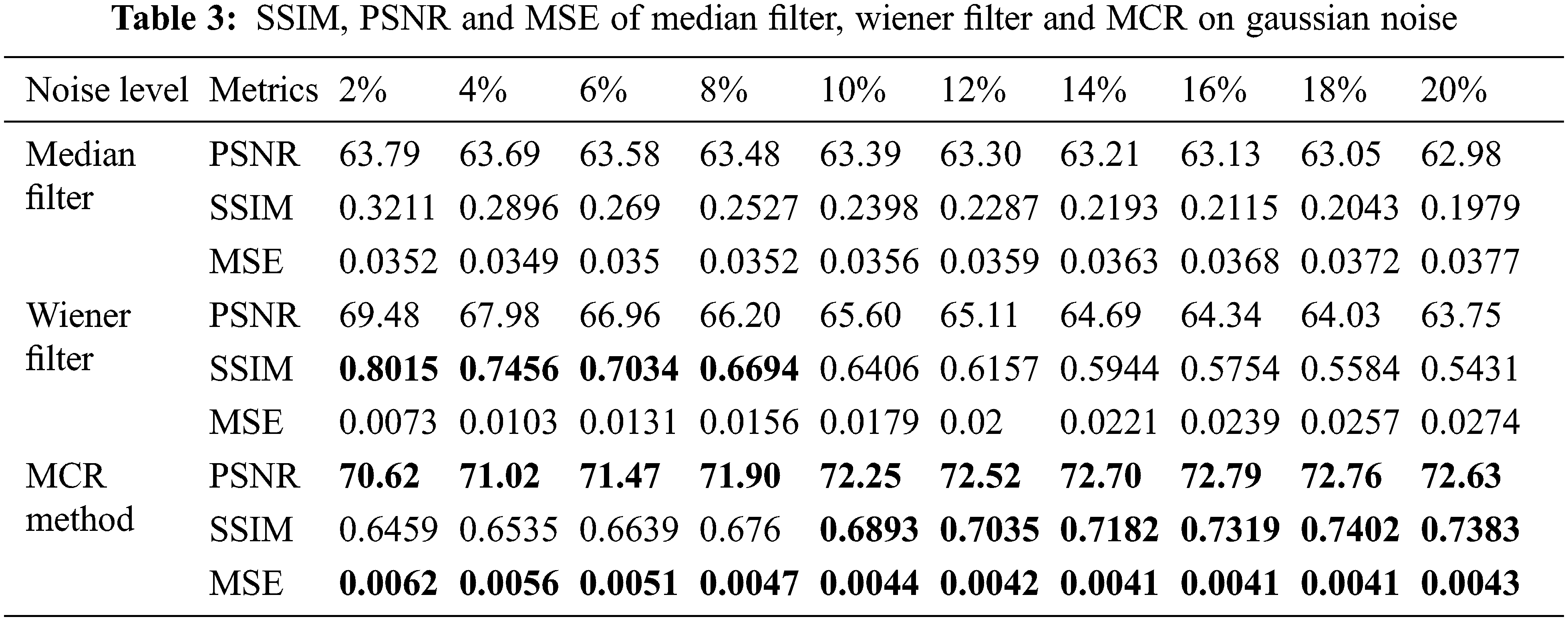
Figure 12: The PSNR, SSIM, and MSE between the clean original and de-noised images by the MCR de-noised method, median filter, and wiener filter for Gaussian noise in rows 1, 2, and 3, respectively

6  Conclusion

This work has developed a de-noising method for brain MR images by mixing two popular deep learning techniques: concatenation and residual learning (MCR). The proposed MCR learning de-noising method successfully cleans the brain images from salt & pepper and Gaussian noise of quantity levels from 2% to 20%. We have used SSIM (Structure Similarity Index), PSNR (Peak Signal-to-Noise Ration), and MSE (Mean Squared Error) to measure the performance of the proposed MCR method. In addition, we have compared our proposed MCR method with two start-of-the-art de-noising filters, median, and Wiener, on salt & pepper and Gaussian noise, both qualitatively and quantitatively in Figs. 9 and 10, and Tabs. 2 and 3. These two types of analysis prove that the MCR de-noising technique is much better than the median and Wiener filters for de-noising the brain MR images for further processing, such as the diagnosis process of brain diseases like bleeding, swelling, tumors, and infections.

Acknowledgement: We appreciate Dr. Adnan N. Qureshi’s supervision throughout this study.

Funding Statement: The authors received no specific funding for this study.

Conflicts of Interest: The authors declare that they have no conflicts of interest to report regarding the present study.

Appendix A. Examples of Denoising Brain MRI Images by Using the MCR Method

Some visual results of the proposed MCR denoising method are represented in Figs. 13 and 14 for removing salt&pepper and Gaussian noises from brain MR images, respectively.

Figure 13: The first row shows the original clean brain MR images, the second row shows the salt & pepper noisy images, and the third row represents the denoised images using the proposed MCR de-noised learning method

Figure 14: The first row shows the original clean brain MR images, the second row shows the noisy Gaussian images, and the third row represents the denoised images using the proposed MCR method

References

1. L. Hirsch, “Magnetic Resonance Imaging (MRIBrain,” 2002, Available: https://kidshealth.org/en/parents/mri-brain.html,. [Google Scholar]
2. P. Kuppusamy, J. Joseph and S. J. B. S. P. Jayaraman, “A customized nonlocal restoration schemes with adaptive strength of smoothening for magnetic resonance images,” Biomed. Signal Process, vol. 49, pp. 160–172, 2019. [Google Scholar]
3. H. V. Bhujle and B. H. J. B. S. P. Vadavadagi, “NLM based magnetic resonance image denoising-A review,” Biomedical Signal Processing and Control, vol. 47, no. 6, pp. 252–261, 2019. [Google Scholar]
4. P. C. Tripathi and S. J. P. R. L. Bag, “CNN-DMRI: A convolutional neural network for denoising of magnetic resonance images,” Pattern Recognition Letters, vol. 135, no. 6, pp. 57–63, 2020. [Google Scholar]
5. G. Gerig, O. Kubler, R. Kikinis and F. A. J. I. T. O. M. I. Jolesz, “Nonlinear anisotropic filtering of MRI data,” IEEE Transactions on Medical Imaging, vol. 11, no. 2, pp. 221–232, 1992. [Google Scholar]
6. J. Sijbers, A. J. den Dekker, A. Van der Linden, M. Verhoye and D. J. M. R. I. V. Dyck, “Adaptive anisotropic noise filtering for magnitude MR data,” Magnetic Resonance Imaging, vol. 17, no. 10, pp. 1533–1539, 1999. [Google Scholar]
7. M. Lysaker, A. Lundervold and X.-C. J. I. T. O. I. P. Tai, “Noise removal using fourth-order partial differential equation with applications to medical magnetic resonance images in space and time,” IEEE Transactions on Image Processing, vol. 12, no. 12, pp. 1579–1590, 2003. [Google Scholar]
8. A. A. Samsonov and C. R. J. M. R. I. M. A. O. J. O. T. I. S. f. M. R. I. M. Johnson, “Noise-adaptive nonlinear diffusion filtering of MR images with spatially varying noise levels,” Magnetic Resonance in Medicine: An Official Journal of the International Society for Magnetic Resonance in Medicine, vol. 52, no. 4, pp. 798–806, 2004. [Google Scholar]
9. K. Krissian and S. J. I. T. O. I. P. Aja-Fernández, “Noise-driven anisotropic diffusion filtering of MRI,” IEEE Transactions on Image Processing, vol. 18, no. 10, pp. 2265–2274, 2009. [Google Scholar]
10. H. M. Golshan, R. P. Hasanzadeh and S. C. J. M. R. I. Yousefzadeh, “An MRI denoising method using image data redundancy and local SNR estimation,” Magnetic resonance imaging, vol. 31, no. 7, pp. 1206–1217, 2013. [Google Scholar]
11. J. C. Wood and K. M. J. M. R. I. M. A. O. J. O. T. I. S. f. M. R. I. M. Johnson, “Wavelet packet denoising of magnetic resonance images: Importance of Rician noise at low SNR,” Magnetic Resonance in Medicine: An Official Journal of the International Society for Magnetic Resonance in Medicine, vol. 41, no. 3, pp. 631–635, 1999. [Google Scholar]
12. A. Pizurica, W. Philips, I. Lemahieu and M. J. I. T. O. M. I. Acheroy, “A versatile wavelet domain noise filtration technique for medical imaging,” IEEE Transactions on Medical Imaging, vol. 22, no. 3, pp. 323–331, 2003. [Google Scholar]
13. J. V. Manjón, P. Coupé, A. Buades, D. L. Collins and M. J. M. I. A. Robles, “New methods for MRI denoising based on sparseness and self-similarity,” Medical Image Analysis, vol. 16, no. 1, pp. 18–27, 2012. [Google Scholar]
14. A. Buades, B. Coll, J.-M. J. M. M. Morel, simulation, “A review of image denoising algorithms, with a new one,” Multiscale Modeling & Simulation, vol. 4, no. 2, pp. 490–530, 2005. [Google Scholar]
15. N. Wiest-Daesslé, S. Prima, P. Coupé, S. P. Morrissey and C. Barillot, “Rician noise removal by non-local means filtering for low signal-to-noise ratio MRI: Applications to DT-MRI,” in Int. Conf. on Medical Image Computing and Computer-assisted Intervention, Newyork, NY, USA, pp. 171–179, 2008. [Google Scholar]
16. P. Coupé, P. Yger, S. Prima, P. Hellier, C. Kervrann et al., “An optimized blockwise nonlocal means denoising filter for 3-D magnetic resonance images,” IEEE transactions on medical Imaging, vol. 27, no. 4, pp. 425–441, 2008. [Google Scholar]
17. P. Coupé, P. Hellier, S. Prima, C. Kervrann and C. J. I. J. O. B. I. Barillot, “3D wavelet subbands mixing for image denoising,” International Journal of Biomedical Imaging, vol. 2008, pp. 1–11, 2008. [Google Scholar]
18. J. V. Manjón, J. Carbonell-Caballero, J. J. Lull, G. García-Martí, L. Martí-Bonmatí et al., “MRI denoising using non-local means,” Medical Image Analysis, vol. 12, no. 4, pp. 514–523, 2008. [Google Scholar]
19. J. V. Manjón, P. Coupé, L. Martí-Bonmatí, D. L. Collins and M. J. J. O. M. R. I. Robles, “Adaptive non-local means denoising of MR images with spatially varying noise levels,” Journal of Magnetic Resonance Imaging, vol. 31, no. 1, pp. 192–203, 2010. [Google Scholar]
20. H. Lv and R. J. I. A. Wang, “Denoising 3D magnetic resonance images based on low-rank tensor approximation with adaptive multirank estimation,” IEEE Access, vol. 7, pp. 85995–86003, 2019. [Google Scholar]
21. Q. Shi, “Domain adaption for fine-grained urban village extraction from satellite images,” IEEE Geoscience and Remote Sensing Letters, vol. 17, no. 8, pp. 1430–1434, 2019. [Google Scholar]
22. H. Guo, “Scene-driven multitask parallel attention network for building extraction in high-resolution remote sensing images,” IEEE Transactions on Geoscience and Remote Sensing, vol. 59, no. 5, pp. 4287–4306, 2020. [Google Scholar]
23. S. Liu, Q. Shi, L. J. I. T. O. G. Zhang and R. Sensing, “Few-shot hyperspectral image classification with unknown classes using multitask deep learning,” IEEE Transactions on Geoscience and Remote Sensing, vol. 59, no. 6, pp. 5085–5102, 2020. [Google Scholar]
24. Q. Shi, X. Tang, T. Yang, R. Liu, L. J. I. T. O. G. Zhang et al., “Hyperspectral image denoising using a 3-D attention denoising network,” IEEE Transactions on Geoscience and Remote Sensing, vol. 59, no. 12, pp. 10348–10363, 2021. [Google Scholar]
25. K. Zhang, W. Zuo and L. J. I. T. O. I. P. Zhang, “FFDNet: Toward a fast and flexible solution for CNN-based image denoising,” IEEE Transactions on Image Processing, vol. 27, no. 9, pp. 4608–4622, 2018. [Google Scholar]
26. K. Song, Q. Ling, Z. Li and F. Li, “An improved MRI denoising algorithm based on wavelet shrinkage,” in The 26th Chinese Control and Decision Conf. (2014 CCDC2014, Changsha, China, pp. 2995–2999, 2014. [Google Scholar]
27. S. Luo and J. Han, “Filtering medical image using adaptive filter,” in 2001 Conf. Proc. of the 23rd Annual Int. Conf. of the IEEE Engineering in Medicine and Biology Society, Istanbul, Turkey, 3, pp. 2727–2729, 2001. [Google Scholar]
28. J. Benesty, J. Chen, Y. A. Huang and S. Doclo, “Study of the Wiener filter for noise reduction,” in Speech Enhancement. Springer, Berlin, Heidelberg, Germany, pp. 9–41, 2005. [Google Scholar]
29. I. S. Isa, S. N. Sulaiman, M. Mustapha and S. J. P. C. S. Darus, “Evaluating denoising performances of fundamental filters for T2-weighted MRI images,” in 19th Int. Conf. on Knowledge Based and Intelligent Information and Engineering Systems. Procedia Computer Science, KES-2015, Singapore, 60, pp. 760–768, 2015. [Google Scholar]
30. C. Szegedy, “Going deeper with convolutions,” in Proc. of the IEEE Conf. on Computer Vision and Pattern Recognition, Boston, MA, USA, pp. 1–9, 2015. [Google Scholar]
31. K. He, X. Zhang, S. Ren and J. Sun, “Deep residual learning for image recognition,” in Proc. of the IEEE Conf. on Computer Vision and Pattern Recognition, Honolulu, Hawaiipp, pp. 770–778, 2016. [Google Scholar]