Brain Tumor: Hybrid Feature Extraction Based on UNet and 3DCNN

1  Introduction

Disease may be described as the uncontrolled, unusual proliferation and division of cells in the body that occurs in the absence of any growth or growth in the environment. An accumulation of abnormal cell formation and division in the cerebrum tissue causes it to get worse and this condition is referred to as brain cancer. In spite of the fact that cerebellar growths are not needlessly abnormal, they are the most lethal illness [1]. Furthermore, they are the most difficult cancers to treat due to their intricacies. In regard to brain tumors, the origin of the tumor decides whether it is classified as a primary or metastatic brain tumor. In contrast to primary brain tumors, which are created from brain tissue cells, metastatic brain tumors are generated when cells from another part of the body become dangerous and move to the cerebrum [2]. Metastatic brain tumors are not as common as primary brain tumors. Primary brain tumors are created when cells derived from brain tissue cells have malignant tendencies and proliferate. Glanzhiomas are a kind of cerebrum growth that arises from the glial cells that coat the surface of the brain. They are not cancerous. Even though they are uncommon, most brain tumor segmentation [3], research is now limited to these particular kinds of brain tumors, which is a severe constraint.

The term “glioma” refers to a broad range of different types of brain tumors, ranging from low-grade gliomas such as oligodendrogliomas and astrocytoma to high-grade glioblastomamultiforme (grade IV), which is the most severe and deadly primary brain cancer in humans. Glanomas are treated using a mix of surgical, chemotherapy, and radiation treatments, all of which are often used in conjunction with one another to provide the best results. In regard to segmenting brain tumors such as glioblastomas and assessing the therapeutic response, Magnetic Resonance Imaging (MRI) is the experimental tool of choice [4]. MRI is a technology that is often utilized by an experienced radiologist to create a succession of pictures (Flair, T1, T1, contrast, T2,…, etc.) to detect separate areas of malignancy. This collection of pictures assists radiologists and other healthcare professionals in obtaining different types of information about the tumor from the photographs they take (shape, volume, etc.). Manual segmentation in Magnetic Resonance Imaging (MRI) is a time-consuming process that is mostly dependent on the expertise of the person doing it [5–7]. The flow diagram of the proposed work is shown in Fig. 1.

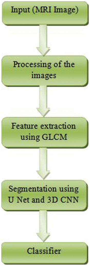
Figure 1: Flow diagram of the proposed method

3D CNN offer a very efficient that can do real-time dense volumetric segmentation in real-time. The 3D multi-fiber unit, comprised of a collection of lightweight 3D convolutional networks, is used to lower the computational burden on the network dramatically. By combining with contextual data, this structure increases the discriminating power of the entire model to segregate tumors with varying sizes. The output of the network is then post-processed using a 3D fully linked Conditional Random Field to produce structural segmentation of appearance and spatial consistency. The SENet module is added to obtain the important degree of each feature channel automatically through the sample-based self-learning, which can improve recognition accuracy with less network parameters growth. A vehicle re-identification model with greater local attention is presented. Branches of the model are global and local at the same time.

The following is the primary contribution of the planned work:

     i)  The Gray-Level Co-event matrix and the Vantage Point Tree are used to pick the elements of the picture, and both have great execution and classifier capabilities.

    ii)  Networks with two segmentations, such as the U-Net and 3D CNN, are proposed for more accurate and better predictions, respectively.

   iii)  The 3D CNN technique is used to more correctly separate the enhancing tumor.

    iv)  The 3D U-Net is employed for the tumor core because it performs better in the sub-region of the final prediction than the 2D U-Net.

The remainder of the paper is organized as follows: Section 2 analysis the related works involved in the brain tumor classification. Section 3 describes the proposed CNN model and how the dataset was used to train and assess the neural network’s performance. Section 4 then analyses the experimental data and results, including a performance comparison with alternative methodologies. Finally, Section 5 concludes the key results of the proposed research.

2  Related Works

As stated by Menze et al. [8], the subject of brain tumor segmentation has attracted a large number of researchers during the last three decades, resulting in an exponential increase in the number of large-scale published publications concerning brain tumor segmentation throughout this period. The present circumstance has for some time been believed to be one where the making of a brilliant mind cancer division system would be an exceptionally desirable solution. More importantly, instead of requiring professionals to spend time on manual diagnosis, this intelligent segmentation technology reduces the amount of time required for the diagnosis procedure to a minimum. In this manner, doctors are given the opportunity to spend more time with their silent over the span of treatment and follow-up. In an attempt to automate this work performed by the radiologist, several studies have been conducted in the past few years (i.e., the restriction and division of the whole growth and its subparts). It is possible to classify these algorithms into two categories: (1) those that computerize the restriction and division of the whole growth and its subareas [9], and (2) those that do not. The recording of many factors related to the tumor’s features is required in order for these models to function, whereas generative models require prior knowledge of the tumor and its tissue and appearance to function. Models that are discriminative [10], on the other hand, become familiar with the quality of a cancer and how to segment it from physically commenting on information without the requirement for extra manual preparation (made by radiologists). The training data required by some algorithms, such as Deep Learning (DL) algorithms, can be rather substantial. Convolutional Neural Networks (CNNs) exhibited their effectiveness as a feature recognition and extraction tool. It was thanks to this technique that we were able to make substantial progress in all computer vision tasks in 2012. When compared to other models, Alexnet a model in view of CNNs created by Tamilvizhi et al. [11], it was proven to generate the best results in picture categorization. Among other things, the AlexNet model is a more complex variant of the LeNet5 [12] model (in that it has a greater number of layers than LeNet5), and a considerable lot of the best models in the PC vision field are extended forms of the AlexNet model, including ZFNet [13], VGGNet [14], GoogleLetNet [15], and RestNet [16] to name a few. Many classic Machine Learning (ML) methods have been outperformed by CNNs in a variety of computer vision applications, including object identification and recognition, among other things [17–20]. The categorization of brain tumors is a more challenging research problem to answer than the classification of brain tumors. The following factors are recognized as contributing to the challenges involved with the situation: The following statements are correct regarding brain tumors: In terms of shape, size, and intensity, they are quite diverse; in terms of appearance, tumors from various disease groups may seem very similar to one another. Among the most frequent forms of pituitary tumor, glioma, brain tumors, and meningiomas are those that account for the vast majority of occurrences.

Cheng et al. [21] explored the three-class brain tumor classification problem using T1-MRI data and found that it was difficult to distinguish between them [22]. This was the first large classification study to use the challenging dataset from fig-share, and it was the first significant classification work to do in the field of classification. To extract characteristics from the region of interest, the proposed technique relied on a tumor boundary that was manually drawn around the region of interest. When developing this study, the authors carried out extensive trials using a broad range of picture features, in addition to a number of classifier models. A Support Vector Machine (SVM) model was able to get the greatest classification performance by incorporating Bag-of Words (BoW) characteristics into its design. Experimental procedures followed a standard five-fold cross-validation technique, which was used for the current study [23]. Performance measures such as sensitivity, specificity, and classification accuracy were measured and compared to one another. Ismael and Abdel-Qadar [24] devised a categorization method based on statistical data acquired from photographs using a Discrete Wavelet Transform (DWT) and a Gabor filter, which they applied to the images. They were then employed in the training and classification of a Multi-Layer Perceptron (MLP) classifier, which was then applied to the data to category. A prior research project had used the fig-shared dataset, and this was the first time the approach had been tried on it. For the training and validation sets, it was chosen to divide the database images into two groups of 70% and 30%, respectively, to establish a training set and a validation set.

In [25], the authors described how to use a CNN-based DL model to the problem of brain cancer classification in an effective manner. In contrast to manually subdividing tumor areas, using CNN-based classifiers offers the benefit of providing a totally automated classification method that eliminates the need for human subdividing. Using data from brain MRI scans, a CNN architecture was built by Pashaei et al. [26] for the purpose of extracting characteristics from the data. Each of the model’s five learnable levels had a filter with a pixel size of 3 × 3 pixels, and all layers contained filters with the same pixel size as the model. According to the CNN model, the accuracy of classification was 81 percent in this case. A classifier model from the area of extreme learning machines was used to increase the performance of the machine by merging CNN features with the model (ELM). According to this study, memory measurements for the class of pituitary tumors were extraordinarily high. However, recall measurements for the class of meningioma were fairly low. This demonstrates that the discriminating capacity of the classifier has significant limitations. Afshar et al. [27] were able to improve the accuracy of brain tumor classification by modifying the CNN design to include a capsule network (CapsNet). CapsNet took use of the spatial connectivity that existed between the tumor and its surrounding tissues. Although this was true, there was only a modest improvement in overall performance. F-measure is an external quality metric usable for quality assessment activities. It leverages the principles of accuracy and recall in information retrieval [28,29]. The clustering technique quality, which could be quantified using the F-measure criterion, was compared. F-measure is an external quality metric suited for quality assessment activities [30]. When extracting the skin lesion, the presence of texture-enhanced dermoscopic pictures with uneven texture patches is a limitation. As a result, a 2D Gaussian filter was used to smooth the data [31]. Meta-heuristic are an iterative generation processes that may lead a heuristic algorithm by diverse responsive notions for exploring and exploiting the search space [32].

Jie et al. [33] classified brain tumors using capsule networks using a Bayesian technique. To enhance tumor identification outcomes, a capsule network was employed instead of a CNN, since CNNs might lose critical spatial information. The Bayes Cap framework was suggested by the team. They utilized a benchmark brain tumor dataset to validate the proposed model. Water molecules in our bodies are normally scattered at random. MRI works by aligning the protons in hydrogen atoms using a magnetic field. A radio wave beam then hits these atoms, causing the protons to spin in a specific way and release small signals that the MRI device picks up. MRI pictures may be generated from these data and then analyzed further. Images of the brain may be generated using this technology. These images might be utilized to determine and analyse the tumor’s shape and size, as well as to determine the best course of therapy for the brain tumor. In a patch-based approach is given in Brain Tumor Analysis and Detection Deep Convolutional Neural Networks (BTADCNN), which addresses the challenge of brain tumor detection in MRI. MRI images are separated into N patches, which are subsequently rebuilt from the individual patches. In the next step, the center pixel label of each patch is calculated using a CNN model that has been previously trained. When all patches have been projected, the total results are added together. Due to the restricted resolution of MR images in the third dimension, each slice is split into a variety of axial views to get the highest possible resolution. The architecture processes each individual 2D slice sequentially, in which every pixel is connected through various MR modalities such as Fluid Attenuation Inversion Recovery (FAIR), Diffusion Weighted Image (DWI), T1 and T1-contrast, spin–spin relaxation, and image modalities such as numerous segmentation methods using CNN.

In [34], an accurate and automated categorization technique for brain tumors has been established in Brain Tumor Classification using CNN (BTCCNN), which distinguishes between the three pathogenic kinds of brain tumors (glioma, meningioma, and pituitary tumor). The deep transfer learning CNN model is used to extract features from the brain MRI images, which are then fed into the solution. To categorize the extracted features, well-known classifiers are employed. Following that, the system is subjected to a thorough examination. When evaluated on the publicly accessible dataset from fig-share, the suggested method outperforms all other comparable methods in terms of classification accuracy. By constructing three Incremental Deep Convolutional Neural Network models that were used for entirely automated segmentation of brain tumors, from beginning to end. These models differ from earlier CNN-based models in that they use a trial and error technique to identify the suitable hyper-parameters rather than a guided strategy to find the appropriate hyper-parameters. Furthermore, ensemble learning is employed to develop a more efficient modelling system. The test of preparing CNN models was tackled by fostering a one-of-a-kind preparation technique that considers the most affecting hyper boundaries by bouncing and laying out a rooftop to these hyper boundaries to speed up the preparation cycle and reduce the training time. In a study titled Brain Tumor Classification and Segmentation Using a Multiscale CNN (BTCSMCNN) [35], MRI images of three types of tumors were analysed over three different views: coronal, sagittal, and axial views. Pre-processing of the pictures was not necessary to eliminate skull or spinal column components from the data. Using publicly available MRI images of 3064 slices from 233 patients, the approach’s performance is compared to that of previously published classical deep learning and machine learning approaches.

Tumor class imbalances are another typical problem. Using data augmentation techniques, this problem is frequently solved by resizing or rotating existing images. Currently, the majority of deep learning algorithms incorporate tumor area classification [36]. However, the network does not know the anatomical location of the tumor region. Images are segmented by breaking them into component segments or regions, which allows for the identification of edges and objects in the images. This splitting is performed on the basis of the image’s pixel properties [37]. Partitioning may be used to separate pixels with similar forms and colours or to group pixels with similar colours and shapes together. Medical imaging relies heavily on image segmentation, which is a common practice. The treatment of disorders of the brain is often considered the most complex. Every year, around 350,000 new cases of brain tumor are recorded globally, and the Five year survival rate for individuals diagnosed with a brain tumor is just 36% [38]. A benign (noncancerous) brain tumor may be malignant (cancerous). Four levels of severity have been established by the WHO for brain tumors. Neurosurgeons often prescribe surgery to treat brain tumors. On the other hand, in the late stages of tumor growth, various procedures such as radiation and chemotherapy are often advocated, because the only approach to diagnose is to try to kill or block the proliferation of malignant cells. Because brain tumors have a high fatality rate, early detection is important for appropriate treatment.

3  The Proposed Hybrid Feature Extraction for Brain Tumor Classification (HFEBTC)

3.1 Grey Level Co-Occurrence Matrix (GLCM)

One of the most common methods for obtaining texture information is the co-occurrence of Grey Levels Matrices [39–42]. An image is represented by a GLCM matrix, which contains the frequency value of the brightness difference between one pixel and its surroundings that occurs in the image. According to the GLCM, the direction q is represented by an angle of (0, 45, 90, and 135). The distance (d) between two pixels specifies the amount of space between them. Fig. 2 depicts a clear definition of direction and distance in terms of arrows.

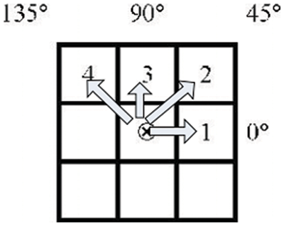
Figure 2: GLCM’s direction and distance

A reference pixel is the center pixel that contains the sign (x). Pixels 1, 2, 3, and 4 and pixel (x) is the same, which means that the distance between them is d = 1. q = 0 is represented by the first pixel, q = 45 is represented by the second pixel, q = 90 is represented by the third pixel, and q = 135 is represented by the fourth pixel. It is necessary to know how far and in which direction you intend to glance before we can calculate GLCM. The following step is to design the matrix framework that will be used in the paper. The grey degree intensity range of the picture is represented by the framework matrix in this image. This framework matrix will now be populated with information about the pixels in the picture that are close to each other. After the occurrence matrix has been filled, the upsides of every element in the matrix are standardized by separating the all-out number of components in the lattice by the absolute number of elements in the matrix. Because the total of all elements in the surrounding matrix equals one, normalizing each component of the matrix can be thought of as a probability function for each member in the nearby matrix [43–46]. The objective is to include all GLCM’s features under a single scope.

3.2 Vantage Point Tree (VPT)

As a result, Vantage Point Trees (VPTs) are created by employing absolute distances between data points from randomly chosen centers to recursively separate the data points (VPTs) [47–52]. At the end of each cycle, these centers, which are referred to as Vantage Points (VPs), divide the data focus and thus around half of them are inside the edge and the other half are outside of the threshold. This offers a framework in which tree neighbours are more likely than not to be spatial neighbours, making the search for them more efficient [53–60]. Fig. 3 portrays a model vantage point tree for a 2D arrangement of focuses, which can be utilized to show the idea. Coming up next are the actions to take: The root hub is relegated to all places in the request wherein they are got. From that point forward, a Vantage Point (R) is chosen indiscriminately (Fig. 3a). The edge is determined and thus the focuses are separated into two equivalent segments (a = 5). d (Point; V P) focuses relocate to the youngster hub on the left (P, S Q), while the leftover focus moves to the kid hub on the right (U, T, V W) (Fig. 3b). The right youngster hub is managed first, trailed by different kids. Arbitrarily chosen VPs (U = 4) are chosen. This is trailed by a shift of all focuses that are d (Point; V P) to the left youngster hub (T) and a shift of the rest of the right (V W) (Fig. 3c). From that point onward, the left kid hub is taken care of along these lines. One of the VPs is picked aimlessly (P a = 6). Following that, all focus that d (Point; V P) shifts to the left youngster hub (S), and the rest of to the right kind hub (Q) of the tree (Fig. 3d). When the intensities of adjacent pixels (I(ui) and I(vj)) are identical, the weighting function has a maximum weight of 1, indicating that the pixels are equally important. It is a free parameter that acts as a length scale for similarity.

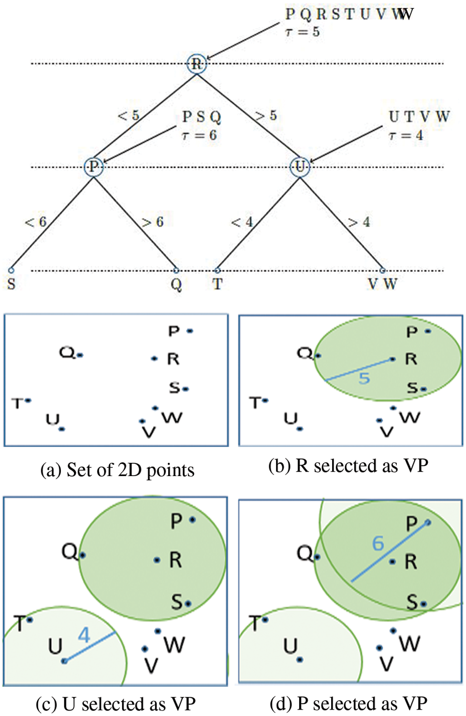
Figure 3: Vantage point tree construction

Consider the metric space ( [−1, 1]d , dist) (d ≥ 1) with a max-distance function in Eq. (1).

dist(u,v)=max1≤i≤d|ui−vi| (1)

Moreover, it is necessary to describe the criteria for selecting the thresholds. It is self-evident that Ih⊂Ih−1 and, additionally, a point x is saved in the left subtree of Th if dist ( x, xTh ) ≤ τh . This gives in Eq. (2).

Ih= Ih−1∩⁡Bτh(xTh),h ≥1 (2)

where Bτh(xTh) is a metric ball of radius τh and center,  xTh , that is in Eq. (3),

Bτh(xTh)={x ∈ χ :dist(x, xTh)≤ τh (3)

3.3 3D CNN

The 3D CNN is an array of three-dimensional CNNs that makes use of a multifibre unit, as shown in Fig. 4, in conjunction with dilated weighted convolutions, to extract feature properties at various scales for volumetric segmentation [61,62]. Pre-processing: Before the data is sent into the network for training, it is upgraded using a variety of approaches to improve its quality (mirroring, rotation, and cropping). Training: The model was prepared with a fixed size of 128 × 128 and an revised loss function, which incorporated both the focused loss with the generalized loss. Inference: According to the interference, the MRI information was zero-cushioned and thus the first 240 240 155 voxels were changed over to 240 240 160 voxels, a profundity for which the organization had the option to part appropriately. Whenever the information is prepared for induction, we send it through the prepared organization, which then, at that point, makes likelihood maps for us. The outfit then, at that point, utilizes these guides to create the last gauge in light of the information.

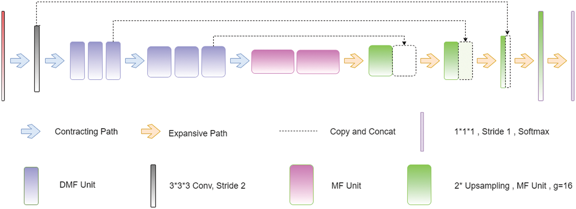
Figure 4: Architecture of 3D CNN

Mathematical expression of the output value γ at position (x, y, z) on the jth feature map in the ith 3D convolutional layer can be written in Eq. (4).

γj,xyzi = ReLU=(bj(i)+ ∑m=1M(i−1)⁡∑u=0U(i)−1⁡∑v=0V(i)−1⁡∑w=0W−1⁡wjm,pqr(i) γm,(x+p)(y+q)(z+r)(i−1)) (4)

where ReLU( ⋅ ) represents elementwise ReLU function; bj(i) is the shared bias for jth process region; wjm,uvw(i) is the (u, v, w)th data of the 3D filter for jth process region at ith layer related with the mth process region in the (i−1)th layer.

Tensor operations may be used to explain simply the link between two neighbouring layers (in this case from (i−1) th to ith, as given in Eq. (5).

γ(i)= σ(W(i)γ(i−1)+b(i)) (5)

where γ(i) and γ(i−1) are the output and input for the ith layer; σ ( ⋅ ) represents the activation function performing element wise;

Loss function is used in back propagation to figure out the training loss. Categorical Cross-entropy was our method of choice. The loss function has to be reduced in order to train the FCN. Stochastic Gradient Descent (SGD) is the most frequent approach for optimizing a model; however it is simpler to become stuck in the gradient trough. As a result, we use the Adam, a method for optimizing the learning rate.

This is the loss function, which is defined as the mean squared error between a 3D-prediction CNN’s and the ground truth of the training dataset in Eq. (6).

L(W,b/D)= 1n∑k=1n⁡∑l=112⁡(ykltruth−yklpred)2 (6)

where D is the trained data set {xk, yk} , represents the quantity of samples, and l signifies the efficient properties vector of the component index. The optimal parameters {W∗andb∗} may be derived by minimizing the loss function, which is the inverse of the loss function in Eq. (7),

{W∗,b∗}=argmin{W,b}{L(W,b/D)} (7)

In DNN-based techniques, a recurring problem is how to limit the fitting that occurs as a result of the DNN’s exceptional approximation capacity.

3.4 3D U-Net

Our group’s subsequent model is a 3D U-Net variety that contrasts with the ordinary U-Net engineering in that the ReLU initiation work is subbed with flawed ReLUs, and case standardization is utilized rather than bunch standardization. The model is worked from the beginning on our dataset and has the comparative design (Fig. 5). During the pre-handling stage, assemble the data important to diminish the size of the MRI cut. Following that, we resample the pictures as well as the generally heterogeneous information’s middle voxel space, after which we perform z-score standardization on the subsequent information. With regard to preparing the organization, we utilize a 128 × 128 × 128 voxel input fix size and a cluster size of 2 to accomplish the best outcomes. A few information increase procedures (gamma amendment, reflecting, and revolution) are applied to the information during runtime to stay away from over fitting and further develop the model’s division exactness while staying away from over fitting. During the induction stage, it utilizes a fix-based technique in which each fix covers a large portion of its size and the voxels nearest to the middle are given a higher load than those farther away.

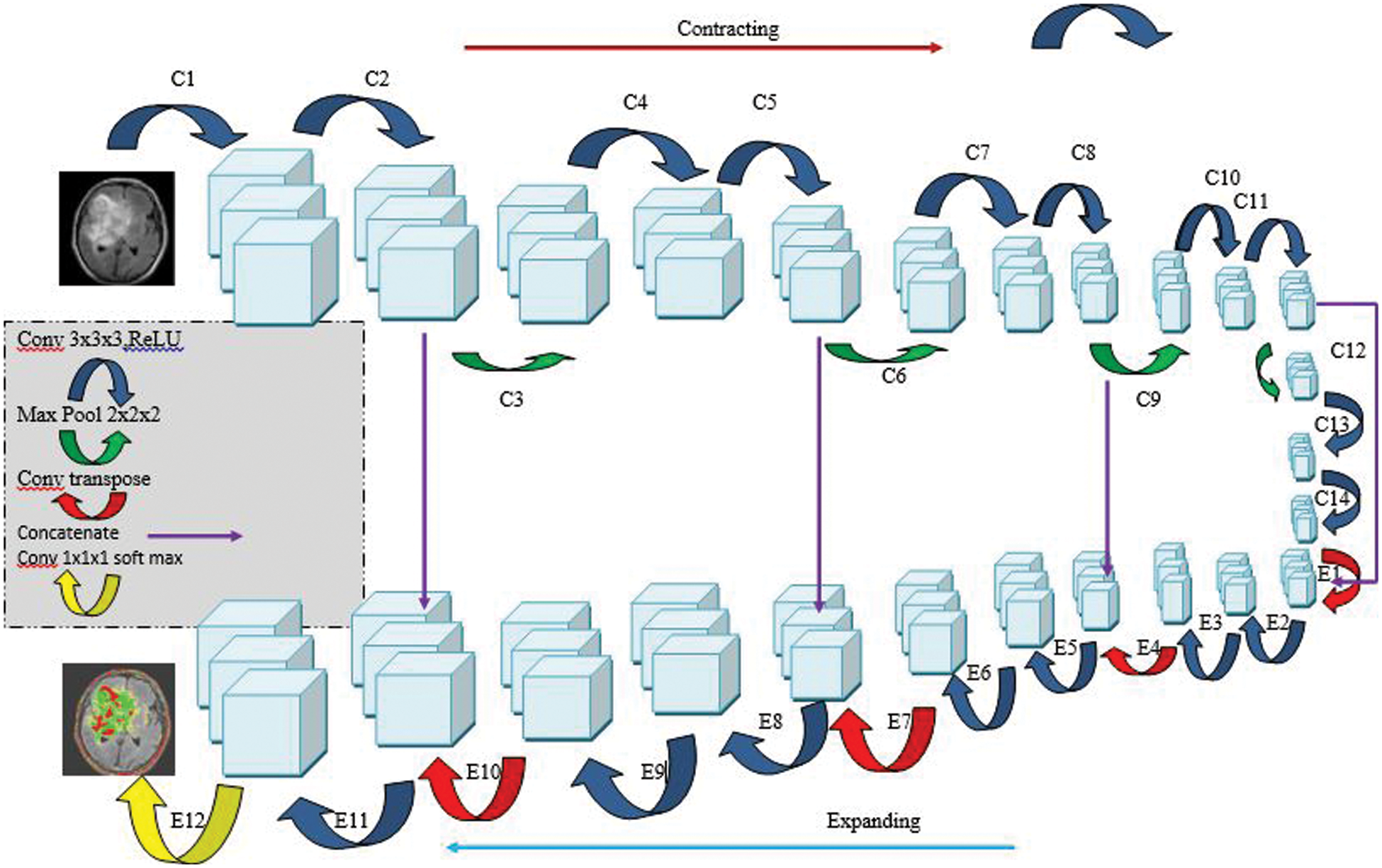
Figure 5: Architecture of 3D U-Net

For each image, the posterior probability of voxel i with label l computation can be written in Eq. (8).

p(yi=l/(Mi))= efyl(Mi)∑k′=1K⁡efyk′(Mi) (8)

where fyi(⋅) is the CNN computation function, Mi is the patch of the voxel i and k’ is the class number.

The weighted cross-entropy loss function is written as follows in Eq. (9).

Loss=−∑i⁡log(p(yi=groundtruth/X(Mi))) (9)

Since the cross-entropy between the actual distribution q and the estimated distribution p is- ∑i⁡q(yi)log(p(yi/X(Mi))) and the actual distribution q(yi) is 1 for ground truth and 0 otherwise. The component extraction phase of the image classification process was the initial step. The element extraction technique utilized was Gray Level Co-event matrix surface element extraction, which was a dim level co-event grid surface element extraction strategy. The GLCM qualities that were utilized were relationship, divergence, homogeneity, differentiation, and energy points (0, 45, 90, and 135). Fig. 6 shows an example of four original MRI images given with the GLCM and VPT. Then it is segmented to detect the brain tumor from the training image. Fig. 6e shows that the proposed method achieves the average dice scores of 18.80, 3.92, and 23.80 for tumor core, Enhanced tumor, and Whole tumor, respectively. With the assistance of VPTs, we can track down the closest neighbors’ files (of the test highlight vectors) and concentrate their names on their marks. This data is utilized to compute the probability of each mark showing up at every framework position in light of the information. Following that, the mark probabilities are interjected in a straight design all through the whole picture. In regard to tumor enhancement, the experimental results, both qualitative and quantitative, indicate that CNN is more effective at segmenting the tumor. Compared to other methods, however, the U-Net is more accurate in terms of tumor core segmentation. However, in regard to finding the entire tumor segmentation on its own, both networks outperform equally well when the expectations are taken into consideration. Consequently, only U-output nets were used to generate the most recent ensemble forecasts for the three regions: We considered the output of both networks to be equal in terms of (1) Tumor Core (TC), (2) Enhancing Tumor (ET), and (3) Whole Tumor value (WT).

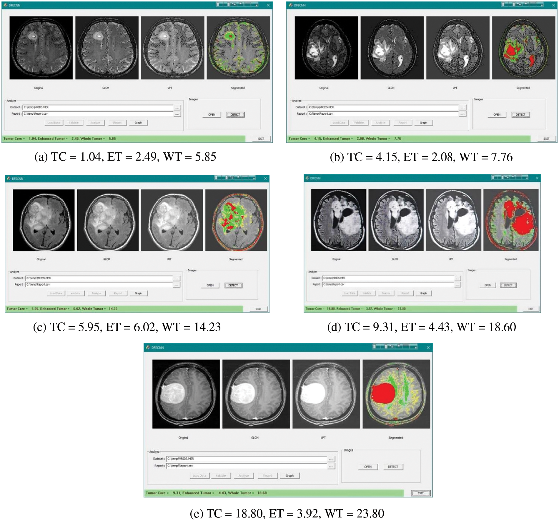
Figure 6: Feature selection of GLCM and VTP along with segmentation for the brain tumor

4  Performance Evaluation

Fig. 7 and Tab. 1 show the comparison of precision in percentage of Enhanced Tumor for the proposed method HFEBTC with the existing methods of “Brain Tumor Analysis and Detection Deep Convolutional Neural Networks” (BTADCNN), “Brain Tumor Classification using CNN” (BTCCNN) and “Brain Tumor Classification and Segmentation Using a Multiscale CNN” (BTCSMCNN). In the proposed method, the precision for Enhanced tumor is 98.51%, which is much higher than the previous existing methods such as 95.952%, 96.785%, and 96.436%.

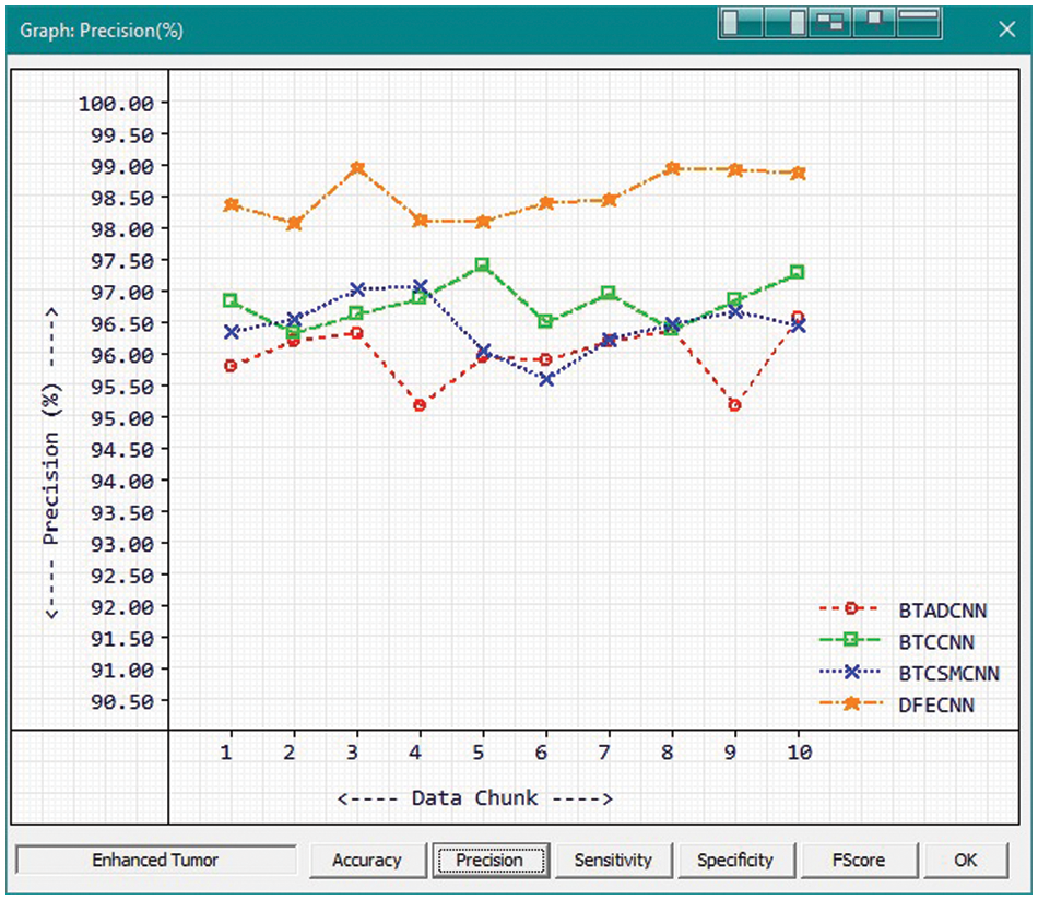
Figure 7: Tumor Type: Enhanced tumor

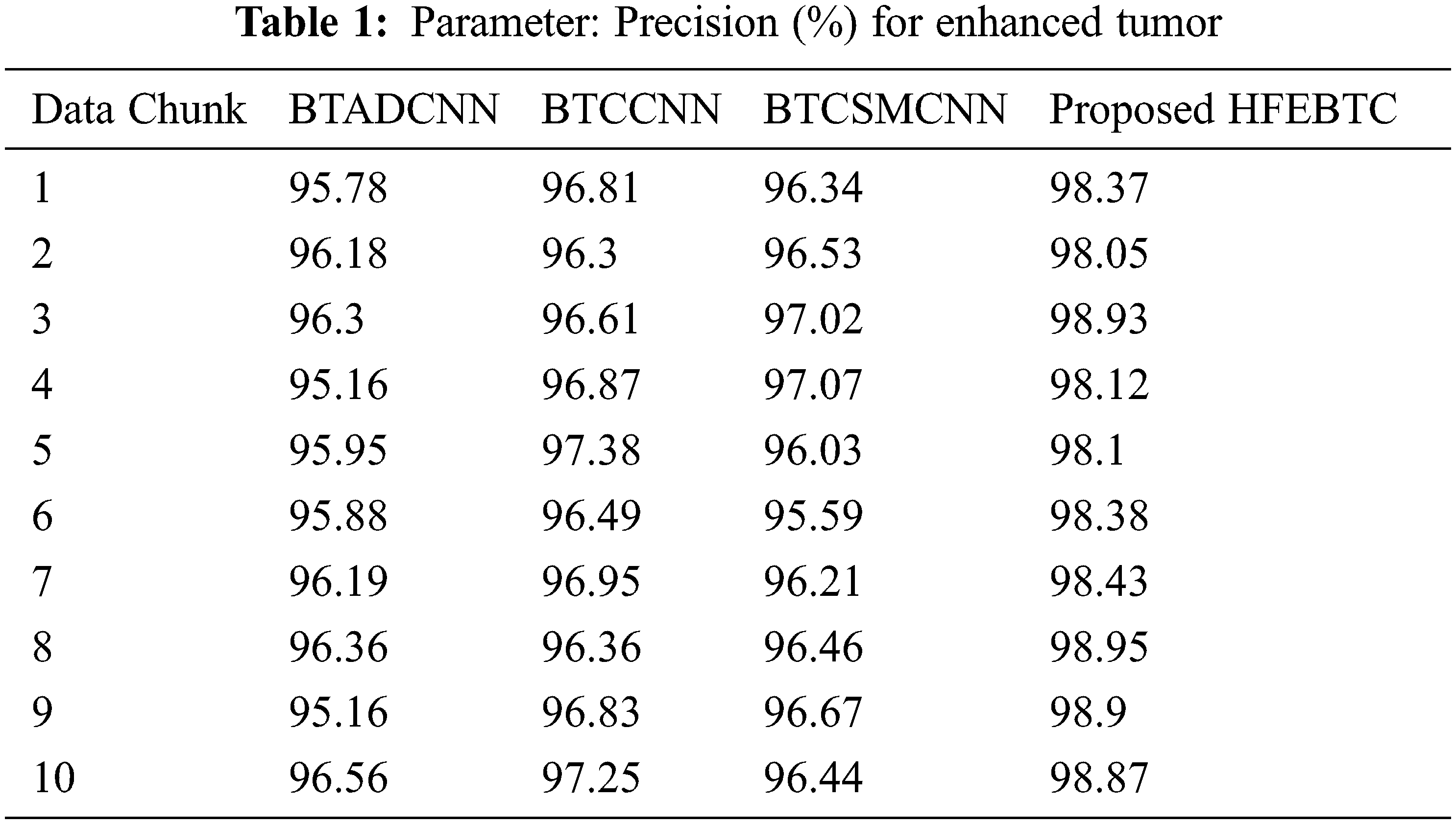
Fig. 8 and Tab. 2 show the comparison of precision in percentage of Tumor core for the proposed method HFEBTC with the existing methods of “Brain Tumor Analysis and Detection Deep Convolutional Neural Networks” (BTADCNN), “Brain Tumor Classification using CNN” (BTCCNN) and “Brain Tumor Classification and Segmentation Using a Multiscale CNN” (BTCSMCNN). In the proposed method, the precision for tumor core is 98.353%, which is much higher than the previous existing methods such as 92.567%, 94.666%, and 97.822%.

Figure 8: Tumor Type: Tumor core

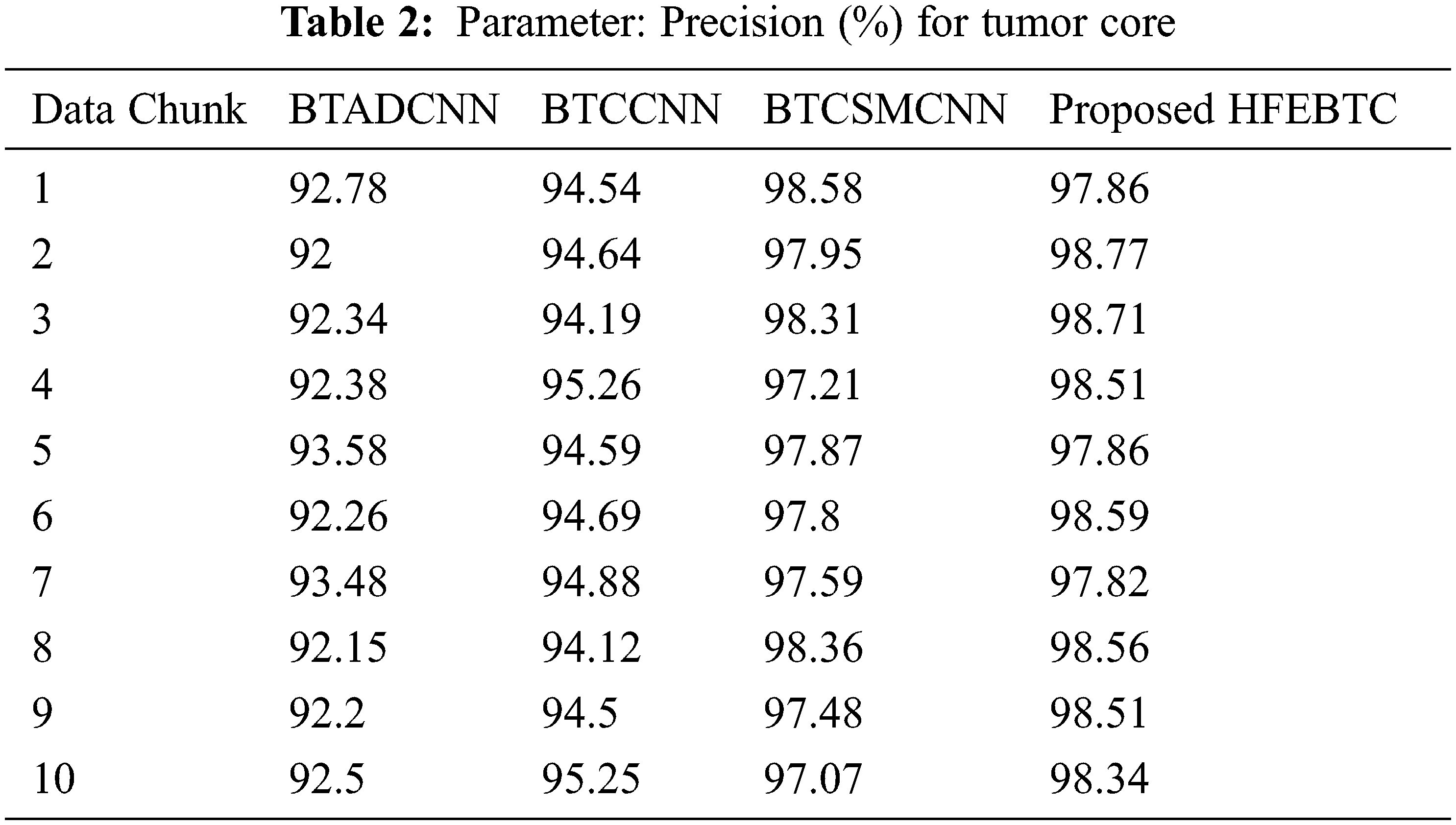
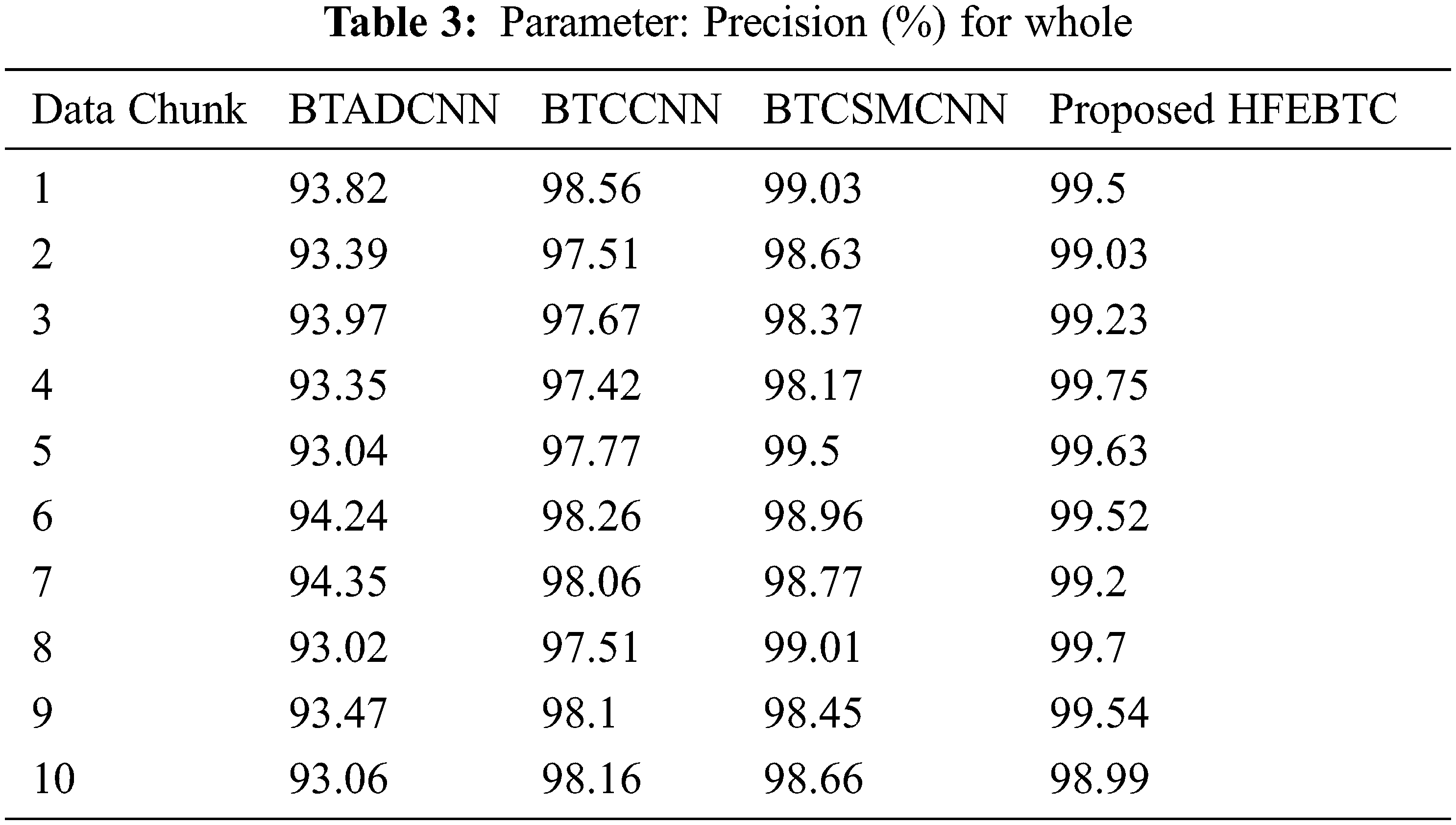
Fig. 9 and Tab. 3 show the comparison of precision in percentage of Tumor core for the proposed method HFEBTC with the existing methods of “Brain Tumor Analysis and Detection Deep Convolutional Neural Networks” (BTADCNN), “Brain Tumor Classification using CNN” (BTCCNN) and “Brain Tumor Classification and Segmentation Using a Multiscale CNN” (BTCSMCNN). In the proposed method, the precision for whole tumor is 99.409%, which is much higher than the previous existing methods such as 93.571%, 97.902%, and 98.755%. When we were attempting to category brain tumors, we compared the performance of our technique to all other methods that were previously available. Tabs. 2 and 3 provide a variety of comparisons based on categorization precision as a metric. The comparison reveals that our technique is superior to any other method currently in use. The suggested technique produced the best results for the tumor core, with 99.409 percent precision. This is to demonstrate how effectively our strategy works despite having a minimal amount of training data compared to previous studies. Because it is utilized in all other works, the table solely displays accuracy as a performance parameter. All measures suggest that the planned work is superior to what is already being done. F-Score values for the enhanced tumor, tumor core and whole tumor are 98.46, 98.29 and 99.40 respectively. Even though the tasks of segmenting brain tumors have been sped up, future research will still face some challenges. We found that the medical images of brain tumor segmentation had an average sparsity of 70% during the study. Better performance can be achieved by utilising the sparse characteristic of the input image in the algorithm or hardware implementation in order to save time spent on invalid computation.

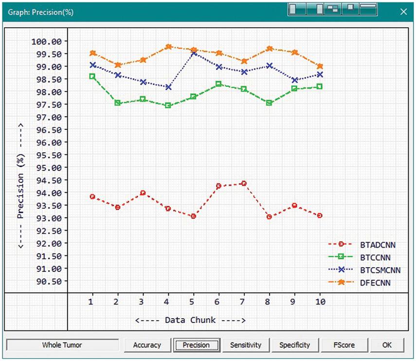
Figure 9: Tumor Type: Whole tumor

5  Conclusion

In the proposed method, the feature extraction of GLCM and VPT was described, as well as the ensemble of two networks. In regard to the challenge of segmentation in biomedical images, both of these networks are frequently used to solve it. The brain tumor ensemble successfully distinguishes brain tumors from normal brain tissue in MRI scans with high accuracy, outperforming forecasts from a wide range of other advanced algorithms. Using a technique known as variable assembling, we aggregate the model’s outputs to achieve the best possible results. The proposed ensemble provides a therapeutically beneficial and automated method for developing brain tumor segmentation for disease planning and patient care that is both efficient and effective. In the proposed method, the precision in percentage for enhanced tumor, tumor core and whole tumor are 98.51%, 98.353% and 99.409% respectively which is much higher than the existing methods. Thus, with these three models, we performed the most state-of-the-art models in terms of precision. As a perspective of this research, we intend to further more experiments on the other parameters like sensitivity, specificity, and F-score.

Acknowledgement: The author would like to thank the Deanship of Scientific Research at Umm Al-Qura University for supporting this work by Grant Code: (22UQU4281755DSR02).

Data Availability Statement: Available Based on Request. The datasets generated and/or analyzed during the current study are not publicly available due to extension of the submitted research work, but are available from the corresponding author on reasonable request.

Funding Statement: This research is funded by Deanship of Scientific Research at Umm Al-Qura University, Grant Code: 22UQU4281768DSR05.

Conflicts of Interest: The authors declare that they have no conflicts of interest to report regarding the present study.

References

 1.  L. M. Deangelis, “Brain tumors,” The New England Journal of Medicine, vol. 344, no. 2, pp. 114–23, 2001. [Google Scholar]

 2.  A. Deimling, “Gliomas,” in Recent Results in Cancer Research, vol. 171, Berlin: Springer, 2009. [Google Scholar]

 3.  R. Stupp, “Malignant glioma: ESMO clinical recommendations for diagnosis, treatment and follow-up,” Annals of Oncology, vol. 18, no. 2, pp. 69–70, 2007. [Google Scholar]

 4.  L. Bangiyev, M. C. R. Espagnet, R. Young, T. Shepherd, E. Knopp et al., “Adult brain tumor imaging: State of the art,” Seminars in Roentgenology, vol. 49, no. 1, pp. 39–52, 2014. [Google Scholar]

 5.  S. J. Chiu, X. T. Li, P. Nicholas, A. T. Cynthia, A. I. Joseph et al., “Automatic segmentation of seven retinal layers in SDOCT images congruent with expert manual segmentation,” Optics Express, vol. 18, no. 18, pp. 19413–19428, 2010. [Google Scholar]

 6.  V. Dill, A. R. Franco and M. S. Pinho, “Automated methods for hippocampus segmentation: The evolution and a review of the state of the art,” Neuroinformatics, vol. 13, no. 2, pp. 133–150, 2015. [Google Scholar]

 7.  L. Shen, H. A. Firpi, A. J. Saykin and D. W. John, “Parametric surface modeling and registration for comparison of manual and automated segmentation of the hippocampus,” Hippocampus, vol. 19, no. 6, pp. 588–595, 2009. [Google Scholar]

 8.  B. H. Menze, A. Jakab, S. Bauer, K. C. Jayashree, F. Keyvan et al., “The multimodal brain tumor image segmentation benchmark (BRATS),” IEEE Transactions on Medical Imaging, vol. 34, no. 10, pp. 1993–2024, 2015. [Google Scholar]

 9.  M. Prastawa, E. Bullitt, S. Ho and G. Gerig, “A brain tumor segmentation framework based on outlier detection,” Medical Image Analysis, vol. 8, no. 3, pp. 275–283, 2004. [Google Scholar]

10. R. Surendran and T. Tamilvizhi, “Cloud of medical things (CoMT) based smart healthcare framework for resource allocation,” in Proc. 3rd Smart Cities Symp. (SCS 2020), Zallaq, Bahrain, pp. 29–34, 2020. [Google Scholar]

11. T. Tamilvizhi, B. Parvathavarthini and R. Surendran, “An improved solution for resource management based on elastic cloud balancing and job shop scheduling,” ARPN Journal of Engineering and Applied Sciences, vol. 10, no. 18, pp. 8205–8210, 2015. [Google Scholar]

12. Y. LeCun, L. Bottou, Y. Bengio and P. Haffner, “Gradient-based learning applied to document recognition,” IEEE, vol. 86, no. 11, pp. 2278–2324, 1998. [Google Scholar]

13. M. D. Zeiler and R. Fergus, “Visualizing and understanding convolutional networks,” in Proc. of the European Conf. on Computer Vision, Springer International Publishing, Switzerland, pp. 818–833, 2014, https://arxiv.org/abs/1311.2901. [Google Scholar]

14. K. Simonyan and A. Zisserman, “Very deep convolutional networks for large-scale image recognition,” arXiv: 1409.1556. http://arxiv.org/abs/1409.1556. 2014. [Google Scholar]

15. C. Szegedy, W. Liu, Y. Jia, S. Pierre, R. Scott et al., “Going deeper with convolutions,” in Proc. of the IEEE Computer Society Conf. on Computer Vision and Pattern Recognition, Boston, MA, pp. 1–9, 2015. https://doi.org/10.1109/CVPR.2015.7298594. [Google Scholar]

16. K. He, X. Zhang, S. Rena and J. Sun, “Deep residual learning for image recognition,” in Proc. of the IEEE Conf. on Computer Vision and Pattern Recognition, Las Vegas, NV, USA, pp. 770–778, 2016. [Google Scholar]

17. Y. Alotaibi and A. Subahi, “New goal-oriented requirements extraction framework for e-health services: A case study of diagnostic testing during the COVID-19 outbreak,” Business Process Management Journal, vol. 28, no. 1, pp. 273–292. 2021. [Google Scholar]

18. R. Girshick, J. Donahue, T. Darrell and J. Malik, “Rich feature hierarchies for accurate object detection and semantic segmentation,” in Proc. of the IEEE Conf. on Computer Vision and Pattern Recognition, Columbus, OH, USA, pp. 580–587, 2014. [Google Scholar]

19. T. Tamilvizhi, R. Surendran, C. A. T. Romero and M. Sadish, “Privacy preserving reliable data transmission in cluster based vehicular adhoc networks,” Intelligent Automation & Soft Computing, vol. 34, no. 2, pp. 1265–1279, 2022. [Google Scholar]

20. D. Anuradha, N. Subramani, O. I. Khalaf, Y. Alotaibi, S. Alghamdi et al., “Chaotic search and rescue optimization based multi-hop data transmission protocol for underwater wireless sensor networks,” Sensors, vol. 22, no. 8, pp. 2867, 2022. [Google Scholar]

21. J. Cheng, W. Huang, S. Cao, Y. Ru, Y. Wei et al., “Enhanced performance of brain tumor classification via tumor region augmentation and partition,” PLoS One, vol. 10, no. 10, pp. e0140381, 2015. [Google Scholar]

22. J. Cheng, W. Yang, M. Huang, H. Wei, J. Jun et al., “Retrieval of brain tumors by adaptive spatial pooling and fisher vector representation,” PLoSOne, vol. 11, no. 6, pp. e0157112, 2016. [Google Scholar]

23. Z. N. K. Swati, Q. Zhao, M. Kabir, A. Farman, A. Zakir et al., “Content-based brain tumor retrieval for MR images using transfer learning,” IEEE Access, vol. 7, pp. 17809–17822, 2019. [Google Scholar]

24. M. R. Ismael and I. Abdel-Qader, “Brain tumor classification via statistical features and back-propagation neural network,” in Proc. of IEEE Int. Conf. on Electro/Information Technology, EIT, Rochester, MI, USA, pp. 252–257, 2018. [Google Scholar]

25. N. Abiwinanda, M. Hanif, S. T. Hesaputra, A. Handayani and T. R. Mengko, “Brain tumor classification using convolutional neural network,” in Proc. of World Congress on Medical Physics and Biomedical Engineering, Springer, Singapore, pp. 183–189, 2018. [Google Scholar]

26. A. Pashaei, H. Sajedi and N. Jazayeri, “Brain tumor classification via convolutional neural network and extreme learning machines,” in Proc. of IEEE 8th Int. Conf. on Computer and Knowledge Engineering, ICCKE, Mashhad, Iran, pp. 314–319, 2018. [Google Scholar]

27. P. Afshar, K. N. Plataniotis and A. Mohammadi, “Capsule networks for brain tumor classification based on MRI images and course tumor boundaries,” in Proc. of IEEE Int. Conf. on Acoustics, Speech and Signal Processing, ICASSP, Brighton, UK, pp. 1368–1372, 2019. [Google Scholar]

28. S. Deepak and P. M. Ameer, “Brain tumor classification using deep CNN features via transfer learning,” Computers in Biology and Medicine, vol. 111, no. pp. 103345, 2019. [Google Scholar]

29. B. Mostefa, S. Rachida, A. Mohamed and K. Rostom, “Fully automatic brain tumor segmentation using end-to-end incremental deep neural networks in MRI images,” Computer Methods and Programs in Biomedicine, vol. 166, pp. 39–49, 2018. [Google Scholar]

30. F. J. Díaz-Pernas, M. Martínez-Zarzuela, M. Antón-Rodríguez and D. González-Ortega. “A deep learning approach for brain tumor classification and segmentation using a multiscale convolutional neural network,” Healthcare (Basel), vol. 9, no. 2, 153, pp. 1–14, 2021. [Google Scholar]

31. L. Guang, L. Fangfang, S. Ashutosh, O. I. Khalaf, A. Youseef et al., “Research on the natural language recognition method based on cluster analysis using neural network,” Mathematical Problems in Engineering, vol. 2021, no. 9982305, pp. 1–13, 2021. [Google Scholar]

32. K. S. Riya, R. Surendran, Carlos Andrés Tavera Romero, M. Sadish Sendil, “Encryption with User Authentication Model for Internet of Medical Things Environment, ” Intelligent Automation & Soft Computing, vol. 35, no. 1, pp. 507–520, 2023. [Google Scholar]

33. X. Jie, H. Jinyan, W. Yuan, K. Deting, Y. Shuo et al., “Hypergraph membrane system based F2 fully convolutional neural network for brain tumor segmentation,” Applied Software Computing, vol. 94, no. 106454, pp. 1–26, 2020. [Google Scholar]

34. R. Amjad, A. K. Muhmmad, S. Tanzila, M. Zahid, T. Usman et al., “Microscopic brain tumor detection and classification using 3D CNN and feature selection architecture,” Microscopy Research and Technique, Wiley Periodicals LLC, pp. 1–17, 2020. [Google Scholar]

35. D. Wu, S. Qinke, W. Miye, Z. Bing and N. Ning, “Deep learning based HCNN and CRF-RRNN model for brain tumor segmentation,” IEEE Access, vol. 8, pp. 26665–26675, 2020. [Google Scholar]

36. S. Rajendran, O. I. Khalaf, Y. Alotaibi and S. Alghamdi, “MapReduce-Based big data classification model using feature subset selection and hyperparameter tuned deep belief network,” Scientific Reports, vol. 11, no. 1, pp. 1–10, 2021. [Google Scholar]

37. S. C. Ekam, H. Ankur, G. Ayush, G. Kanav and S. Adwitya, “Deep learning model for brain tumor segmentation and analysis,” in Proc. 3rd Int. Conf. on Recent Developments in Control, Automation and Power Engineering (RDCAPE), IEEE, Noida, India, 2019. [Google Scholar]

38. T. Tahia, S. Sraboni, G. Punit, I. A. Fozayel, I. Sumaia et al., “A robust and novel approach for brain tumor classification using convolutional neural network,” Computational Intelligence and Neuroscience, vol. 2021, no. 2392395, pp. 1–11, 2021. [Google Scholar]

39. R. Rout, P. Parida, Y. Alotaibi, S. Alghamdi and O. I. Khalaf, “Skin lesion extraction using multiscale morphological local variance reconstruction based watershed transform and fast fuzzy C-means clustering,” Symmetry, vol. 13, no. 2085, pp. 1–19, 2021. [Google Scholar]

40. V. Ramasamy, Y. Alotaibi, O. I. Khalaf, P. Samui and J. Jayabalan, “Prediction of groundwater table for chennai region using soft computing techniques,” Arabian Journal of Geosciences, vol. 15, no. 9, pp. 1–19, 2022. [Google Scholar]

41. Y. Alotaibi, “A new meta-heuristics data clustering algorithm based on tabu search and adaptive search memory,” Symmetry, vol. 14, no. 3, 623, pp. 1–15, 2022. [Google Scholar]

42. A. O. Kingsley, R. Surendran and O. I. Khalaf, “Optimal artificial intelligence based automated skin lesion detection and classification model,” Computer Systems Science and Engineering, vol. 44, no. 1, pp. 693–707, 2023. [Google Scholar]

43. G. Suryanarayana, K. Chandran, O. I. Khalaf, Y. Alotaibi, A. Alsufyani et al., “Accurate magnetic resonance image super-resolution using deep networks and Gaussian filtering in the stationary wavelet domain,” IEEE Access, vol. 9, pp. 71406–71417, 2021. [Google Scholar]

44. S. S. Rawat, S. Alghamdi, G. Kumar, Y. Alotaibi, O. I. Khalaf et al., “Infrared small target detection based on partial sum minimization and total variation,” Mathematics, vol. 10, no. 671, pp. 1–19, 2022. [Google Scholar]

45. P. Mohan, N. Subramani, Y. Alotaibi, S. Alghamdi, O. I. Khalaf et al., “Improved metaheuristics-based clustering with multihoprouting protocol for underwater wireless sensor networks,” Sensors, vol. 22, no. 4, pp. 1618, 2022. [Google Scholar]

46. N. Subramani, P. Mohan, Y. Alotaibi, S. Alghamdi and O. I. Khalaf, “An efficient metaheuristic-based clustering with routing protocol for underwater wireless sensor networks,” Sensors, vol. 22, no. 415, pp. 1–16, 2022. [Google Scholar]

47. S. Bharany, S. Sharma, S. Badotra, O. I. Khalaf, Y. Alotaibi et al., “Energy-efficient clustering scheme for flying ad-hoc networks using an optimized LEACH protocol,” Energies, vol. 14, no. 19, pp. 6016, 2021. [Google Scholar]

48. A. Alsufyani, Y. Alotaibi, A. O. Almagrabi, S. A. Alghamdi and N. Alsufyani, “Optimized intelligent data management framework for a cyber-physical system for computational applications,” Complex & Intelligent Systems, pp. 1–13, 2021. [Google Scholar]

49. Y. Alotaibi, M. N. Malik, H. H. Khan, A. Batool, S. U. Islam et al., “Suggestion mining from opinionated text of big social media data,” Computers, Materials & Continua, vol. 68, no. 3, pp. 3323–3338, 2021. [Google Scholar]

50. Y. Alotaibi, “A new database intrusion detection approach based on hybrid meta-heuristics,” Computers, Materials & Continua, vol. 66, no. 2, pp. 1879–1895, 2021. [Google Scholar]

51. S. R. Akhila, Y. Alotaibi, O. I. Khalaf and S. Alghamdi, “Authentication and resource allocation strategies during handoff for 5G IoVs using deep learning,” Energies, vol. 15, no. 6, pp. 2006, 2022. [Google Scholar]

52. S. Sennan, D. Pandey, Y. Alotaibi and S. Alghamdi, “A novel convolutional neural networks based spinach classification and recognition system,” Computers, Materials & Continua, vol. 73, no. 1, pp. 343–361, 2022. [Google Scholar]

53. S. Sennan, G. Kirubasri, Y. Alotaibi, D. Pandey and S. Alghamdi, “Eacr-leach: Energy-aware cluster-based routing protocol for wsn based IoT,” Computers, Materials & Continua, vol. 72, no. 2, pp. 2159–2174, 2022. [Google Scholar]

54. A. Sundas, S. Badotra, Y. Alotaibi, S. Alghamdi and O. I. Khalaf, “Modified bat algorithm for optimal VM’s in cloud computing,” Computers, Materials & Continua, vol. 72, no. 2, pp. 2877–2894, 2022. [Google Scholar]

55. P. Kollapudi, S. Alghamdi, N. Veeraiah, Y. Alotaibi, S. Thotakura et al., “A new method for scene classification from the remote sensing images,” Computers, Materials & Continua, vol. 72, no. 1, pp. 1339–1355, 2022. [Google Scholar]

56. A. R. Khaparde, F. Alassery, A. Kumar, Y. Alotaibi, O. I. Khalaf et al., “Differential evolution algorithm with hierarchical fair competition model,” Intelligent Automation & Soft Computing, vol. 33, no. 2, pp. 1045–1062, 2022. [Google Scholar]

57. H. S. Gill, O. I. Khalaf, Y. Alotaibi, S. Alghamdi and F. Alassery, “Fruit image classification using deep learning,” Computers, Materials & Continua, vol. 71, no. 3, pp. 5135–5150, 2022. [Google Scholar]

58. H. S. Gill, O. I. Khalaf, Y. Alotaibi, S. Alghamdi and F. Alassery, “Multi-model CNN-RNN-LSTM based fruit recognition and classification,” Intelligent Automation & Soft Computing, vol. 33, no. 1, pp. 637–650, 2022. [Google Scholar]

59. S. Alqazzaz, X. Sun, X. Yang and L. Nokes, “Automated brain tumor segmentation on multi-modal MR image using SegNet,” Computational Visual Media, vol. 5, no. 2305, pp. 209–219, 2019. [Google Scholar]

60. Z. Zhou, Z. He and Y. Jia, “AFPNet: A 3D fully convolutional neural network with atrous-convolution feature pyramid for brain tumor segmentation via MRI images,” Neurocomputing, vol. 402, pp. 235–244, 2020. [Google Scholar]

61. W. Sun, G. Zhang, X. Zhang, X. Zhang and N. Ge, “Fine-grained vehicle type classification using lightweight convolutional neural network with feature optimization and joint learning strategy,” Multimedia Tools and Applications, vol. 80, pp. 30803–30816, 2021. [Google Scholar]

62. W. Sun, X. Chen, X. Zhang, G. Dai, P. Chang et al., “A multi-feature learning model with enhanced local attention for vehicle re-identification,” Computers,” Materials & Continua, vol. 69, no. 3, pp. 3549–3561, 2021. [Google Scholar]