Attribute Reduction for Information Systems via Strength of Rules and Similarity Matrix

1  Introduction

Pawlak proposed Rough set theory (RST) in 1982 [1]. RST is considered as a powerful mathematical research technique in pattern recognition, machine learning, information discovery, and other fields. Because Pawlak’s RST requires rigid equivalence relations, it can only extract expertise in information systems with definite attributes [2]. Some researchers have extended Pawlak’s idea by incorporating fuzzy equivalence relations, neighborhood relations and dominance relations into Pawlak rough sets to form neighborhood rough sets [3,4], fuzzy rough sets [5–9], and dominance-based rough sets [10–12]. The generalized models of rough set are commonly applied in the reduction of attributes [13–15], feature selection [16–19], extraction of rules [20–23], theory of decisions [24–26], incremental learning [27–29], Collaborative Filtering [30], Variable Precision Rough Set Model, [31], topological rough application [32], reduction in multi-valued information system [33] and so on. A significant application of RST is in the reduction of attributes in databases (feature selection). Given a dataset with distinct attribute values, the reduction of attributes finds subsets having the same attributes as the original. Its principle can be regarded as the most powerful result of RST, differentiating it from other theories. The reduction of attributes for selecting subsets attributes picks detailed and compact attributes and excludes redundant and inconsistent attributes from the learning tasks. Several algorithms for attribute reduction exist based on classical rough sets, rough neighborhood sets, entropy, and mutual knowledge. This study introduces the reduction of attributes using classical RST. Additionally, we introduce the strength of rules and similarity matrix that are also used in reducing attributes. Finally, we discuss many examples to explain these methods. This article is organized as the following: Section 2 provides a quick overview of the fundamental notion of the theory of rough sets and describes the reduction of attributes following the indiscernibility relation and discernibility matrix. Section 3 presents the definition of the strength of rules and some measures for evaluating attributes and discusses their properties. In Section 4, we introduce the definition of similarity matrix for finding the reduct of a decision information table. Finally, Section 5 provides the conclusion.

Fig. 1 presents four methods of reduction of attributes in information systems, which will be discussed in the following sections.

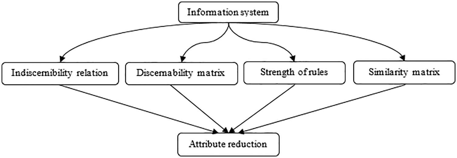
Figure 1: Some methods of attribute reduction in information systems

2  Basic Concepts

2.1 Rough Sets

In the early 1980s, RST was introduced by Pawlak as a new mathematical tool for dealing with uncertainty and vagueness [2]. It is a mathematical technique that may be used for intelligent data analysis. Suppose a system of information

IS=(U,A)

where Universe U and Attributes A are finite nonempty sets.

Set A consists of two distinct sets of attributes called: Condition C and Decision D attributes.

IS=(U,C,D) denotes the system of information.

For every P⊆A,X⊆U,x∈U , we can define the Upper approximations P(X)¯and Lower approximation, {P(X)_, as follows:

P(X)¯=∪{P(x):P(x)∩X≠∅}

and

P(X)_=∪{P(x):P(x)⊆X}

where P(x)={y∈U|xPy} is the equivalence class that contains x according to P .

The boundary region BP(X) is:

BP(X)=P(X)¯−P(X)_

If the boundary region is nonempty, then the set is rough; otherwise, the set is crisp. The ratio of lower- and upper-approximation is used to compute the approximation accuracy of the set X from the elementary subsets. Most of these concepts illustrated in Fig. 2.

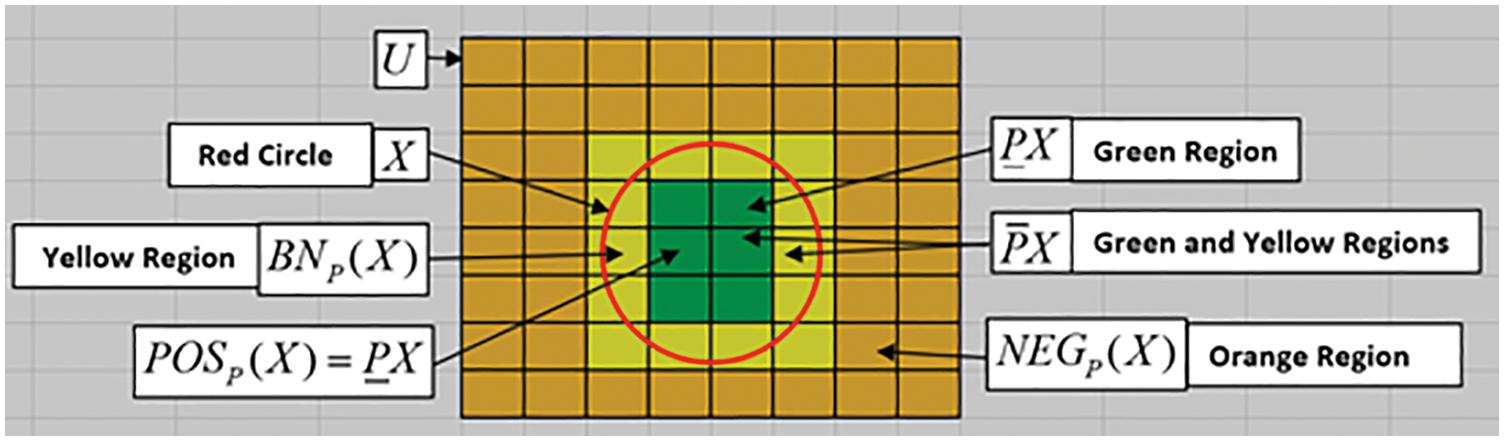
Figure 2: Rough set concepts

Definition 1. The degree of dependency: The degree of dependency: Attributes are divided into condition attributes C and decision attributes D. The degree of dependency denoted as μ(C,D) is defined as [2]

μ(C,D)=|LOW(C,D)|/|U|

where

LOW(C,D)=∪Yi∈U/IND(D)⁡{X∈U/IND(C),X⊆Yi},

which is determined as the union of the equivalence classes of the relation U/IND(C) that are totally contained in one of the equivalence classes of relation U/IND(D) . By definition: 0≤μ(C,D)≤1

2.2 Reduction of Condition Attributes Using Indiscernibility Relation

For every set of condition attributes A⊆C , an indiscernibility relation IND(A) is defined as follows [2]:

Two objects x i and x j are indiscernible by the set of condition attributes, if x i and x j have the same value of condition attributes A⊆C (i.e., a(x i ) = a(x j ) for every a∈A )

More formally,

IND(A)={(xi,xj)∈U2:∀a∈A,a(xi)=a(xj)}

IND(A) is an equivalence relation that partitions U into elementary sets. The partitions induced by IND(A) are equivalence classes and represent the smallest discernible groups of objects using the information contained within. The notation U/A denotes the partitions induced by IND(A) or the elementary sets of the universe U in the space [2].

Example 1.

In the following car information table, see Tab. 1: V: vibration, N: noise, I: interior, C: capacity.

We can obtain the indiscernibility relation from Tab. 1:

1) First, we find the equivalence classes of all attributes dented by U/A.

U/A = {{ c 1} , { c 2} , { c 3} , { c 4} , { c 5} , { c 6} , { c 7} , { c 8}}

2) Second, we find the equivalence classes for each attribute alone.

U/{C} = {{ c 1 ,c 3 ,c 4} , { c 2 ,c 6 ,c 7} , { c 5 ,c 8}}

U/{I} = {{ c 1 ,c 2 ,c 4 ,c 5} , { c 3 ,c 7 ,c 8} , { c 6}}

U/{N} = {{ c 1 ,c 2 ,c 3 ,c 5} , { c 4 ,c 6 ,c 7 ,c 8}}

U/{V} = {{ c 1 ,c 2 ,c 3 ,c 6} , { c 4 ,c 5 ,c 7 ,c 8}}

3) Third, we find the equivalence classes of double attributes only.

U/{C,I} = {{ c 1 ,c 4} , { c 2} , { c 3} , { c 5} , { c 6} , { c 7} , { c 8}}

U/{C,N} = {{ c 1 ,c 3} , { c 2} , { c 4} , { c 5} , { c 6 ,c 7} , { c 8}}

U/{C,V} = {{ c 1 ,c 3} , { c 2 ,c 6} , { c 4} , { c 5 ,c 8} , { c 7}}

U/{I,N} = {{ c 1 ,c 2 ,c 5} , { c 3} , { c 4} , { c 6} , { c 7 ,c 8}}

U/{I,V} = {{ c 1 ,c 2} , { c 3} , { c 4 ,c 5} , { c 6} , { c 7 ,c 8}}

U/{N,V} = {{ c 1 ,c 2 ,c 3} , { c 4 ,c 7 ,c 8} , { c 5} , { c 6}}

4) Fourth, we find the equivalence classes of triple attributes only.

U/{C,I,N} = {{ c 1} , { c 2} , { c 3} , { c 4} , { c 5} , { c 6} , { c 7} , { c 8}}

U/{C,I,V} = {{ c 1} , { c 2} , { c 3} , { c 4} , { c 5} , { c 6} , { c 7} , { c 8}}

U/{C,N,V} = {{ c 1 ,c 3} , { c 2} , { c 4} , { c 5} , { c 6} , { c 7 ,c 8}}

U/{I,N,V} = {{ c 1 ,c 2} , { c 3} , { c 4} , { c 5} , { c 6} , { c 7 ,c 8}}

From the previous relationships, we conclude that.

U/A = U/{C,I,N} and U/A = U/{C,I,V}

Therefore, attribute V or N can be dispensed with.

2.3 Reduction of Condition Attributes Using Discernibility Matrix

Definition 2. Relative Discernibility Matrix

If C and D denote condition and decision attributes respectively. Then the relative discernibility function [2] is given as;

fCD=∧{∨a:a∈MCD≠∅},

where MCD (x,y) = {a ∈C : a(x) ≠ a(y), D(x) ≠ D(y)}

which is used for the reduction of condition attributes relative to decision attributes.

Example 2.

In the following Car decision table Tab. 2: V: vibration, N: noise, I: interior, C: capacity, D: quality.

We obtain the relative discernibility matrix from Tab. 3:

Then; fCD = { N+V } . { C+V } . { C+I+N } . { C+I+N+V } . { C+I+N+V } . { N+V } . { C+V } . { I+N } . { I+N+V } . { C+I+N+V } . { I+N+V } . { C+I+V } . { C+I+N } . { C+N+V } . { C+N+V } . { C+I+V } . { C+I } . { C+I } . { C+I+N+V } . { C+I+N } . { I+N }

= { N+V } .C+V } . { I+N } . { C+I }

= { N.C+V } . { N.C+I } = N.C+V.I

→ REDD(c)=fCD = { { N,C } , { V,I } }

We reduce Tab. 4 by merging different rows which contain the same values for condition and decision attributes, this technique is known as row reduction:

To find the core of each example, we proceed with Tab. 5: in a manner the table remains consistent. By eliminating V = M, we have two decision values L and H. This means that, depending on the attribute V, we are unable to make unique decisions, then V is unable to be removed. Similarly, eliminating N = L leaves two decision values M and H, implying that no unique decision can be made based on attribute N. Thus, the value of N is unable to be removed. Therefor Tab. 5 becomes as follows:

Tab. 6 presents the core of each car.

We delete the repeated rows, as in Tab. 7,

Tab. 7 contains the decision rules since no further reduction is allowed. The following are the decision rules based on the reduction and core:

1) If N(Medium) and V(Medium) ⇒ D(Low)

2) If V(Low) ⇒ D(Medium)

3) If N(Low) ⇒ D(High)

3  Reduction of Condition Attributes Using the Strength of Rules

The rules are now generated based on the reduct and core. The reduced set of relations that maintains the same inductive relation categorization is known as a reduct. If P is minimum and the indiscernibility relation provided by P and Q is the same, the set P of attributes is the reduct of another set Q. The core is described as follows:

Core = ∩ reduct

Definition 3. The strength of rules

Let IS=(U,C,D) be a decision table. Every x∈U determines a sequence c1 (x), …,cn (x), d1(x)……dm((x), where {c1,...,cn}=C and {d1,...,dn}=D . The sequence called the decision rule induced by x in U and denoted by

c1(x),...,cn(x)→d1(x),...,dm(x) or C→xD.

Then the strength of rules is

σ∝,β(Ci,Dj)=|Ci(x)∝∩Dj(x)β||Dj(x)β|,

where Ci(x)∝=∪{x∈U|Ci(x)=α} , Dj(x)β=∪{x∈U|Dj(x)=β} , α∈valuesofCi , β∈valuesofDj , i=1,2,3,…n is the index of condition attributes, and j =1,2,3,…,m is the index of decision attribute.

Example 3.

From Tab. 2, and using Definition 3, we can calculate the strength of rules for all attributes as the following steps:

The rules strength for attribute C may be found as follows:

(C = 5) → (D = Low); the strength of this particular rule = 23 = 66.667%

(C = 4) → (D = Low); the strength of this particular rule = 13 = 33.333%

(C = 5) → (D = Medium); the strength of this particular rule = 12 = 50%

(C = 2) → (D = Medium); the strength of this particular rule = 12 = 50%

(C = 4) → (D = High); the strength of this particular rule = 23 = 66.667%

(C = 2) → (D = High); the strength of this particular rule = 13 = 33.333%

The average of the strength of rules for attribute C = 50%

The rules strength for attribute I may be found as follows:

(I = Fair) → (D = Low); the strength of this particular rule = 23 = 66.667%

(I = Good) → (D = Low); the strength of this particular rule = 13 = 33.333%

(I = Fair) → (D = Medium); the strength of this particular rule = 22 = 100%

(I = Excellent) → (D = High); the strength of this particular rule = 13 = 33.333%

(I = Good) → (D = High); the strength of this particular rule = 23 = 66.667%

The average of the strength of rules for attribute I = 60 %

The rules strength for attribute N may be found as follows:

(N = Medium) → (D = Low); the strength of this particular rule = 33 = 100%

(N = Low) → (D = Medium); the strength of this particular rule = 12 = 50%

(N = Medium) → (D = Medium); the strength of this particular rule = 12 = 50%

(N = Low) → (D = High); the strength of this particular rule = 33 = 100%

The average of the strength of rules for attribute N = 75%

The rules strength for attribute V may be found as follows:

(V = Medium) → (D = Low); the strength of this particular rule = 33 = 100%

(V = Low) → (D = Medium); the strength of this particular rule = 22 = 100%

(V = Medium) → (D = High); the strength of this particular rule= 13 = 33.333%

(V = Low) → (D = High); the strength of this particular rule = 23 = 66.667%

The average of the strength of rules for attribute V = 75%

Note: The attributes with the highest percentage of the strength of rules are N and V, and attributes with fewer proportions can be deleted. The reduct of set { C, I, N, V } is { N, V } . Therefore, Tab. 2 can be reduced to Tab. 8.

Reduce Tab. 8: to become as Tab. 9 by removing the repeated rows of attribute values.

We find the core of Tab. 9; to keep the table consistent. Two decision values L and H remain if we eliminate V = M. This implies that we cannot make a sole judgment based on attribute V, so the value of V cannot be removed. Similarly, two decision values M and H remain when we eliminate N = L, implying that we cannot make a unique judgment based on attribute N. Therefore, the value of N cannot be removed. Now Tab. 9 is like Tab. 10.

Tab. 10: Displays each instance’s core. Tab. 10 can be further reduced; by merging double rows.

By removing the same rows again, we obtain Tab. 11.

Tab. 11 provides us with rules of judgment. No further reduction is necessary. The decisions on reduction and core are as follows.

1) If N(Medium) and V(Medium) ⇒ D(Low)

2) If V(Low) ⇒ D(Medium)

3) If N(Low) ⇒ D(High)

4  Reduction of Condition Attributes Using Similarity Matrix

The similarity matrix is considered a novel method reducing condition attributes. It is easy to use and produces more accurate results, depending on the deletion or dispensing of the attribute that has the least influence on decision making under specific conditions.

Definition 4. Let IS=(U,C,D) be a decision table; then the distance d(xi,xj) between two objects xi,xj∈U according to one attribute a∈A can be calculated using the following equation:

d(xi,xj)={0,xi(a)≠xj(a),a∈A1,xi(a)=xj(a),a∈A

The ratio of the similarity between two objects denoted by δ(xi,xj) is given by the following equation:

δ(xi,xj)=∑d(xi,xj)|A|

Example 4.

From Tab. 2, and Definition 4, we obtain the similarity matrix for all objects as in Tab. 12:

From Tab. 2; we can find the indiscernibility relation of the decision attribute as follows:

U/IND(D) = {{c1,c2,c3},{c4,c5},{c6,c7,c8}}

From Tab. 12, selecting the ratio of similarity between two objects when δ(xi,xj)=1 according to the following equation: f(xi)={xj:δ(xi,xj)=1} ,

we get;

f(c1)={ c 1} , f(c2)={ c 2} , f(c3)={ c 3} , f(c4)={ c 4} , f(c5)={ c 5} , f(c6)={ c 6} , f(c7)={ c 7} , f(c8)={ c 8} ,

→ LOW (U(A)/D) = { c 1 ,c 2 ,c 3 ,c 4 ,c 5 ,c 6 ,c 7 ,c 8}

Then the degree of dependency is

μ(U(A)/D) ) = 88=1

By eliminating attribute C from Tab. 2, we obtain the following similarity matrix in Tab. 13.

From Tab. 13, selecting the ratio of similarity between two objects in the same manner as above, we get;

f(c1)={ c 1 ,c 2},f(c2)={ c 1 ,c 2},f(c3)={ c3},f(c4)={c4} , f(c5)={ c 5},f(c6)={ c 6},f(c7)= {c7 ,c 8},f(c8)={c7} , {c8}

→ LOW (U(A-{C})/D = { c 1 ,c 2 ,c 3 ,c 4 ,c 5 ,c 6 ,c 7 ,c 8}

Then The degree of dependency is

μ(U(A−{C})/D) = 88=1

Also, by eliminating attributes {I}, {N}, {V, {C, N}, {I, V}, {C, I}, {C, V}, {I, N}, {N, V} from Tab. 2 respectively, and computing its similarity matrices, we get the following degree of dependencies:

μ(U(A)/D) = 88 = 88=1

μ(U(A−{C})/D) = 88 = 88=1

μ(U(A−{I})/D) = 88 = 88=1

μ(U(A−{N})/D) = 88 = 88=1

μ(U(A−{V})/D) = 88 = 88=1

μ(U(A−{C,N})/D) = 88 = 88=1

μ(U(A−{I,V})/D) = 88=1

μ(U(A−{I,C})/D) = 58=0.625

μ(U(A−{V,C})/D) = 58=0.625

μ(U(A−{I,N})/D) = 48=0.5

μ(U(A−{N,V})/D) = 68=0.75

From previous calculations, we have;

μ(U(A)/D) =1

μ(U(A−{N,C})/D) =1

μ(U(A−{I,V})/D) =1

Therefore, the reduct(A) = {{ C,N } , { I,V }} .

5  Conclusions

We emphasised in our research the need of decreasing the size of the dataset before beginning any research and how rough set theory provides an effective approach for determining the minimal dataset’s reduct. We also discussed how the rough set may be unable to discover the minimal reduct by itself since doing so may need computing all combinations of attributes, which is not achievable in huge datasets. We proposed two methods to find the reduct of a dataset. One of them is the strength of rules which calculate the strength of rules for all attributes, and the other is similarity matrix, which is considered a novel method reducing condition attributes, it is easy to use and produce more accurate results.

Availability of Data and Materials: The datasets used and analyzed during the current study are public and available from the corresponding author on request.

Authors’ Contributions: The authors declare that they contributed equally to all sections of the paper. All authors read and approved the final manuscript.

Funding Statement: The authors declare that they did not receive third-party funding for the preparation of this paper.

Conflicts of Interest: The authors declare that they have no conflicts of interest to report regarding the present study.

References

1. Z. Pawlak, “Rough sets,” International Journal of Computer & Information Sciences, vol. 11, no. 5, pp. 314–356, 1982. [Google Scholar]
2. Z. Pawlak, Rough Sets-theoretical Aspects of Reasoning about Data, Dordrecht, Boston, London: Kluwer Academic Publishers, 1991. [Google Scholar]
3. Y. Y. Yao, “Relational interpretations of neighborhood operators and rough set approximation operators,” Information Sciences, vol. 111, no. 1–4, pp. 239–259, 1998. [Google Scholar]
4. Y. Y. Yao, “Rough sets, neighborhood systems and granular computing,” in IEEE Canadian Conf. on Electrical and Computer, Canada, pp. 1553–1558, 1999. [Google Scholar]
5. A. Mohammed, A. J. Carlos, A. Hussain and G. Abdu, “On some types of covering-based e, m-fuzzy rough sets and their applications,” Journal of Mathematics, vol. 2021, pp. 1–18, 2021. [Google Scholar]
6. D. Dubois and H. Prade, “Putting rough sets and fuzzy sets together, intelligent decision support,” In: R. Slowinski (Ed.Handbook of Applications and Advances of the Rough Set Theory, Springer, Dordrecht, pp. 203–232, 1992. [Google Scholar]
7. D. Dubois and H. Prade, “Rough fuzzy sets and fuzzy rough sets,” International Journal of General Systems, vol. 17, no. 2–3, pp. 191–209, 1990. [Google Scholar]
8. E. C. C. Tsang, D. Chen, D. S. Yeung, X. Z. Wang and J. W. T. Lee, “Attributes reduction using fuzzy rough sets,” IEEE Transactions on Fuzzy Systems, vol. 16, no. 5, pp. 1130–1141, 2008. [Google Scholar]
9. W. Wu, M. Shao and X. Wang, “Using single axioms to characterize (S, T)-intuitionistic fuzzy rough approximation operators,” International Journal of Machine Learning and Cybernetics, vol. 10, no. 1, pp. 2742, 2019. [Google Scholar]
10. S. Greco, B. Matarazzo and R. Slowinski, “Rough approximation by dominance relations,” International. Journal of Intelligent Systems, vol. 17, no. 2, pp. 153–171, 2002. [Google Scholar]
11. W. Xu, Y. Li and X. Liao, “Approaches to attribute reductions based on rough set and matrix computation in inconsistent ordered information systems,” Knowledge-Based Systems, vol. 27, no. 4, pp. 78–91, 2012. [Google Scholar]
12. A. H. Attia, A. S. Sherif and G. S. El-Tawel, “Maximal limited similarity-based rough set model,” Soft Computing, vol. 20, no. 8, pp. 31–53, 2016. [Google Scholar]
13. D. Chen, L. Zhang, S. Zhao, Q. Hu and P. Zhu, “A novel algorithm for finding reducts with fuzzy rough sets,” IEEE Transactions on Fuzzy Systems, vol. 20, no. 2, pp. 385–389, 2012. [Google Scholar]
14. L. Chen, D. Chen and H. Wang, “Fuzzy kernel alignment with application to attribute reduction of heterogeneous data,” IEEE Transactions on Fuzzy Systems, vol. 27, no. 7, pp. 1469–1478, 2019. [Google Scholar]
15. C. Wang, Y. Huang, M. Shao and X. Fan, “Fuzzy rough set-based attribute reduction using distance measures,” Knowledge-Based Systems, vol. 164, no. 12, pp. 205–212, 2019. [Google Scholar]
16. A. Mirkhan and N. Çelebi, “Binary representation of polar bear algorithm for feature selection,” Computer Systems Science and Engineering, vol. 43, no. 2, pp. 767–783, 2022. [Google Scholar]
17. R. S. Latha, B. Saravana Balaji, N. Bacanin, I. Strumberger, M. Zivkovic et al., “Feature selection using grey wolf optimization with random differential grouping,” Computer Systems Science and Engineering, vol. 43, no. 1, pp. 317–332, 2022. [Google Scholar]
18. U. Ramakrishnan and N. Nachimuthu, “An enhanced memetic algorithm for feature selection in big data analytics with mapreduce,” Intelligent Automation & Soft Computing, vol. 31, no. 3, pp. 1547–1559, 2022. [Google Scholar]
19. R. M. Devi, M. Premkumar, P. Jangir, B. S. Kumar, D. Alrowaili et al., “BHGSO: Binary hunger games search optimization algorithm for feature selection problem,” Computers, Materials & Continua, vol. 70, no. 1, pp. 557–579, 2022. [Google Scholar]
20. X. Zhang, C. Mei, D. Chen and J. Li, “Feature selection in mixed data: A method using a novel fuzzy rough set-based information entropy,” Pattern Recognition, vol. 56, pp. 1–15, 2016. [Google Scholar]
21. X. Zhang, C. Mei, D. Chen, Y. Yang and J. Li, “Active incremental feature selection using a fuzzy-rough-set-based information entropy,” IEEE Transactions on Fuzzy Systems, vol. 28, no. 5, pp. 901–915, 2019. [Google Scholar]
22. D. Chen, W. Zhang, D. Yeung and E. C. C. Tsang, “Rough approximations on a complete completely distributive lattice with applications to generalized rough sets,” Information Sciences, vol. 176, no. 13, pp. 1829–1848, 2006. [Google Scholar]
23. C. Luo, T. Li, H. Chen and D. Liu, “Incremental approaches for updating approximations in set-valued ordered information systems,” Knowledge-Based Systems, vol. 50, no. 50, pp. 218–233, 2013. [Google Scholar]
24. C. Zaibin and M. Lingling, “Some new covering-based multigranulation fuzzy rough sets and corresponding application in multicriteria decision making,” Journal of Mathematics, vol. 2021, pp. 1–25, 2021. [Google Scholar]
25. Y. Guo, E. C. C. Tsang, M. Hu, X. Lin, D. Chen et al., “Incremental updating approximations for double-quantitative decision-theoretic rough sets with the variation of objects,” Knowledge-Based Systems, vol. 189, no. 5, pp. 1–30, 2020. [Google Scholar]
26. S. A. Alblowi, M. E. Sayed and M. A. E. Safty, “Decision making based on fuzzy soft sets and its application in COVID-19,” Intelligent Automation & Soft Computing, vol. 30, no. 3, pp. 961–972, 2021. [Google Scholar]
27. Y. Guo, E. C. C. Tsang, W. Xu and C. Degang, “Local logical disjunction double quantitative rough sets,” Information Sciences, vol. 500, no. 2–3, pp. 87–112, 2019. [Google Scholar]
28. C. Luo, T. Li, H. Chen, H. Fujita and Z. Yi, “Incremental rough set approach for hierarchical multicriteria classification,” Information Sciences, vol. 429, pp. 72–87, 2018. [Google Scholar]
29. C. Luo, T. Li, Y. Huang and H. Fujitad, “Updating three-way decisions in incomplete multi-scale information systems,” Knowledge-Based Systems, vol. 476, pp. 274–289, 2019. [Google Scholar]
30. C. R. Kumar and V. E. Jayanthi, “A novel fuzzy rough sets theory based CF recommendation system,” Computer Systems Science & Engineering, vol. 34, no. 3, pp. 123–129, 2019. [Google Scholar]
31. A. F. Oliva, F. M. Pérez, J. V. B. Martinez and M. A. Ortega, “Non-deterministic outlier detection method based on the variable precision rough set model,” Computer Systems Science and Engineering, vol. 34, no. 3, pp. 131–144, 2019. [Google Scholar]
32. A. S. Salama, “Sequences of topological near open and near closed sets with rough applications,” Filomat, vol. 34, no. 1, pp. 51–58, 2020. [Google Scholar]
33. A. S. Salama, “Bitopological approximation space with application to data reduction in multi-valued information systems,” Filomat, vol. 34, no. 1, pp. 99–110, 2020. [Google Scholar]
Cite This Article
Copyright © 2023 The Author(s). Published by Tech Science Press.
This work is licensed under a Creative Commons Attribution 4.0 International License , which permits unrestricted use, distribution, and reproduction in any medium, provided the original work is properly cited.
Downloads
Citation Tools