Heterogeneous Ensemble Feature Selection Model (HEFSM) for Big Data Analytics

1  Introduction

IS (Intelligent Systems) have been growing rapidly in recent years encompassing the areas of commerce, science and medicine [1]. DM (Data Mining) defined in short as knowledge explorations identify trends, patterns and relationships in data and convert raw data into meaningful information [1]. AI (Artificial Intelligence) based techniques have been useful in normalizing incomplete DM datasets. DMTs (DM techniques) have been exploited in business decisions and organizational priorities. DM tasks include pre-processing, pattern assessments and presentations [2] using Cluster analysis, Time-series mining, ARM (Association Rules Mining) and classifications [3]. Thus, classification techniques play the underlying role in all DM tasks. Classifications grow in complexity when it involves high dimensional data like Big data where dimension is referred to the number of parameter values taken into consideration. As this count increases it increases the computational time required for processing where dimensionality reductions of the data is executed to increase the speed of the processing techniques.

Feature Selection is an efficient method of dimensionality reductions [4]. These selections select a subset with required features from the base set based on an evaluation criteria. The results thus better learning performances in terms of accuracy or classifications. These selections search for minimal representation of features and evaluate thus selected subsets in classification performances [5]. Feature selection methods also contribute towards generalizations of classifiers [6]. These approaches are oriented towards redundancy minimizations and relevance maximizations of labelling classes for classifications. The selected feature subsets retain their original forms and offer better readability and interpretability. When information is labelled, it helps in distinguishing relevant features. Thus these methods can be categorized into supervised, unsupervised and semi-supervised methods for feature selections [7].

Supervised Feature Selections can be viewed as filters, wrappers and embeddings in modelling systems [8,9]. Filters separate unwanted features for classifiers to learn while wrappers use predictive accuracies of previous learning for selecting quality features in data sets. Wrappers are expensive in their executions where metaheuristic algorithms reduce these computational times reasonably. Most metaheuristic algorithms have a problem of getting caught in a local optimum. Evolutionary algorithms have helped overcome this problem in their operations where PSO, GA (Genetic Algorithm), DD (Differential Development), ACO (Ant Colony Optimization), GWO and EHO algorithms are examples in this category. Hybrid techniques aim to use individual algorithmic powers for increased explorations [10].

This paper proposes a new hybrid wrapper for feature selection using FWGWO (Fuzzy Weight Grey Wolf Optimization) and EHO algorithms. Features are selected based on a fuzzy weight that minimizes the subset’s length and increases classification accuracy in parallel. The proposed HEFSM uses multiple algorithms. TCM (Tent Chaotic Map) is the wrapper used to jump local optima while optimizing search capabilities. FWGWO is an easy to implement algorithm which operates with fewer parameters. The algorithm considers location of individual wolves for its solutions. Thus, this work uses EHO in updating positional locations. A binary transformation normalizes continuous features which are then classified by the KNN classifier.

2  Literature Review

Consider Sharawi et al. [11] used WOA (Whale Optimization Algorithm) in their proposed feature selection system. Their meta-heuristic optimization algorithm mimicked the behavior of humpback whales. The proposed model applies the wrapper-based method to reach the optimal subset of features. They compared their technique with the PSO and GA algorithms on sixteen different datasets with multiple parameters. Experimental results demonstrate the proposed algorithm’s ability to optimize feature selections.

Sayed et al. [12] embedded a chaotic search in WOA iterations. Their scheme called CWOA (Chaotic Whale Optimization Algorithm) used TCM’s for improving WOA outputs. Their chaotic exploration operators outperformed other similar techniques. PSO was proposed by Chen et al. [13] in their HPSO-SSM (Hybrid Particle Swarm Optimization with a Spiral-Shaped Mechanism) selected optimal feature subsets for classification using wrappers. Their experimental results showed good performance in searching feature feasibility by selecting informative attributes for classifications.

PSO variant was used by Gu et al. [14] in their study which proposed CSO (Competitive Swarm Optimize) for large-scale optimizations of features in high-dimensional data. Their experimental results of six benchmark datasets showed a better performance than PSO based algorithms. Their CSO selected lesser number of features which could be classified better. Tu et al. [15] proposed HSGWO (Hierarchy Strengthened GWO) as their feature selection technique where wolves were classified as omega and dominant. The technique’s learning used dominant wolves to prevent low ranked wolves and improve cumulative efficiency. This is followed by a hybrid GWO and DE (Differential Evolution) strategy for omega wolves to evade local optimums. Their use of a perturbed operator improved exploration of the diverse population. Their results proved the algorithm’s superiority in convergences and solution quality.

Dimensions were learnt by Haiz et al. [16] with a generalized learning on PSO selected features. They included cardinality of subsets by extending dimension velocity. Their 2D-learning framework retained key features of PSO selections while learning dimensions. When evaluated with NB (Naive–Bayes) and KNN classifications their feature subsets ran faster evaluating its usefulness.

GWO was combined with Antlion Optimization in the study of Zawbaa et al. [17]. The scheme called ALO-GWO (Antlion Optimization -Grey Wolf Optimization) algorithm learnt from fewer examples and used it to select important features from large sets that could improve classification accuracy. The proposal showed promising results in comparison with PSO and GA. APSO (Accelerated Particle Swarm Optimization) proposed by Fong et al. [18] was a lightweight feature selection technique. It was designed specifically for mining streamed data for achieving enhanced analytical accuracy with lesser processing time. The scheme when tested on high dimensionality sets showed its improved performance.

Two-phase Mutation figured in the study of Abdel-Basset et al. [19] based on GWO algorithm. They selected features with wrappers. Their sigmoid function transformed search spaces into a binary form for feature selections. Statistical analysis proved the technique’s effectiveness. Li et al. [20] integrated GWO with a Kernel Extreme Learning Machine in their study. Their framework called (IGWO-KELM) was applied in medical diagnostics. GWO and GA were evaluated in its comparisons for predicting common diseases. Their performance metrics showed improvements in classification accuracy, sensitivity, specificity, precision, G-mean, F-measure and selected feature sizes. GWSO’s binary variant was exploited by ElHasnony et al. [21] in their study. Their technique called GWO-PSO found optimal solutions and used KNN for classifications on wrapper selected features where Euclidean separation matrices found optimal solutions.

Wang et al. [22] proposed a new technique SA-EFS (Sort aggregation-Ensemble Feature Selection) for high-dimensional datasets. The technique used Chi-Square, maximum information coefficient and XGBoost for aggregations. They integrated arithmetic and geometric mean aggregations for analyzing classification and predictive performances of the technique’s selected feature subsets. Their experimental results showed arithmetic mean aggregation ensemble feature selections effectively improved classification accuracy and that threshold intervals of 0.1 performed better. An empirical study in Pes [23] included many types of selection algorithms in different application domains. Eighteen heterogeneous classification tasks were evaluated with different cardinality feature subsets where ensemble approaches performed better even on single selectors.

Despite numerous attempts to develop an efficient model for characteristic choice in Big Data applications, the complexity of handling such data remains a significant barrier. As a result of the large volume and intricacy of large data sets, the data mining operation may be hampered. The characteristic choice method is a required pre-processing phase to reduce dataset dimensionality for the most useful characteristics and categorization performance improvement. It takes time to conduct a comprehensive analysis for important traits. In this paper, a new Heterogeneous Ensemble Feature Selection Model) which includes several algorithms in a hybrid combination is proposed. To determine the best answers, a K-nearest neighbour classifier with Euclidean separation matrices is utilised.

3  Proposed HEFSM Methodology

This work proposes feature selections based on sorted aggregations using ensembles in its approach. Three feature selection methods are executed in HEFSM to obtain multiple optimal feature subsets. Filtering is done by ReliefF, InfoG (Information Gain), and GR (Gain Ratio) methods. The proposed work also embeds SVM-t (Support Vector Machine- t-statistics). A new binary variant of wrappers based on the FWGWO and EHO is used in feature selections. Individual outputs of the used methods are learnt based on rules for getting multiple optimal feature subset candidate sets which are then aggregated to produce optimized feature subsets. The proposed algorithm of this work is verified using KNN classification. Fig. 1 depicts the flow of this research work.

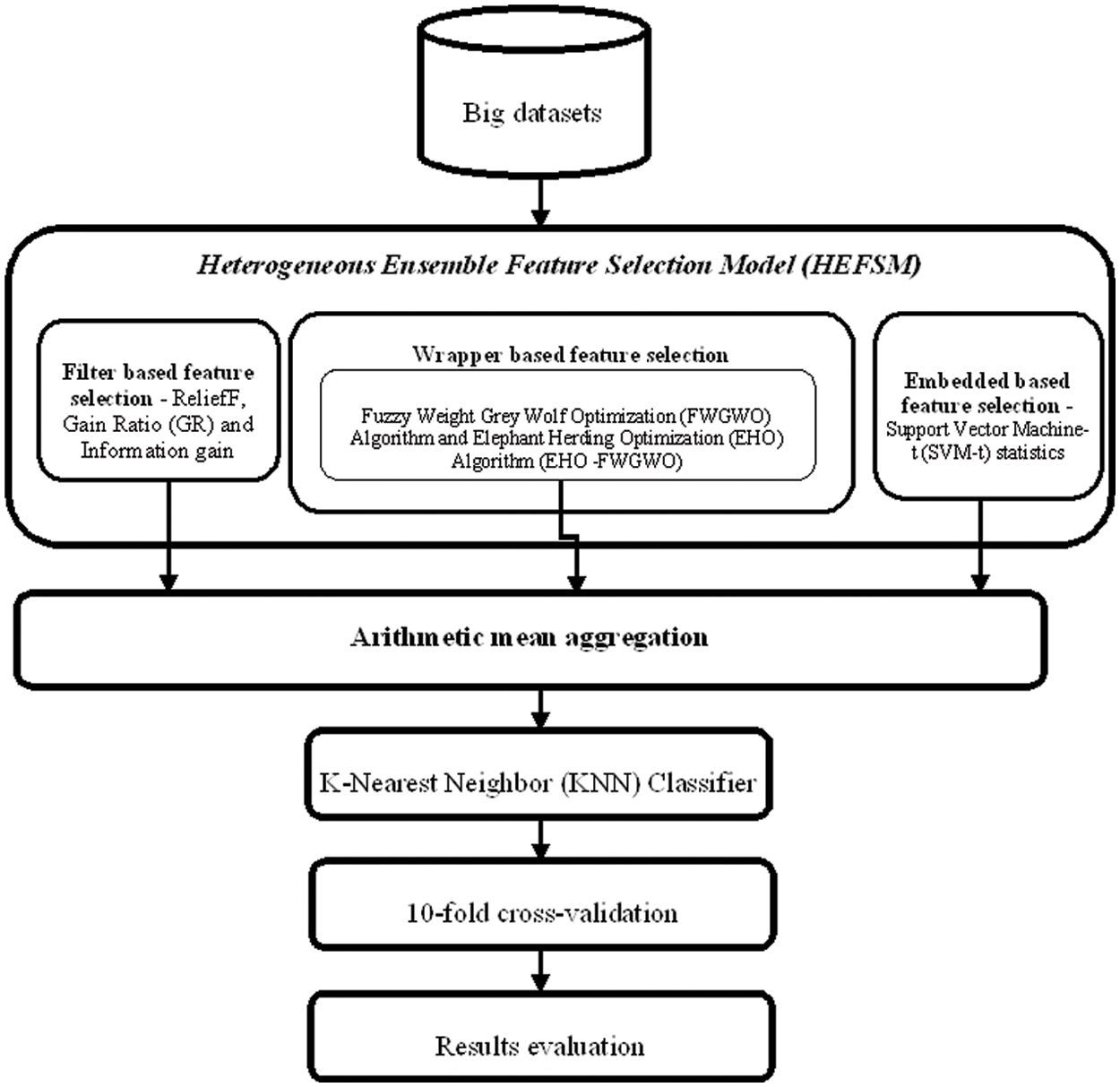
Figure 1: Flow of the proposed system

3.1 HEFSM

Ensembles learn better in ML by combining different ML learning models [24,25]. They are better than singular ML models as they effectively output multiple optimal features. Hence, this work uses ensembles for better feature selections by using combinations of filters, wrappers and an embedded algorithm.

3.1.1 Filters

Data Filtering in this work are based on three functions namely ReliefF, InfoG, and GR [25].

ReliefF

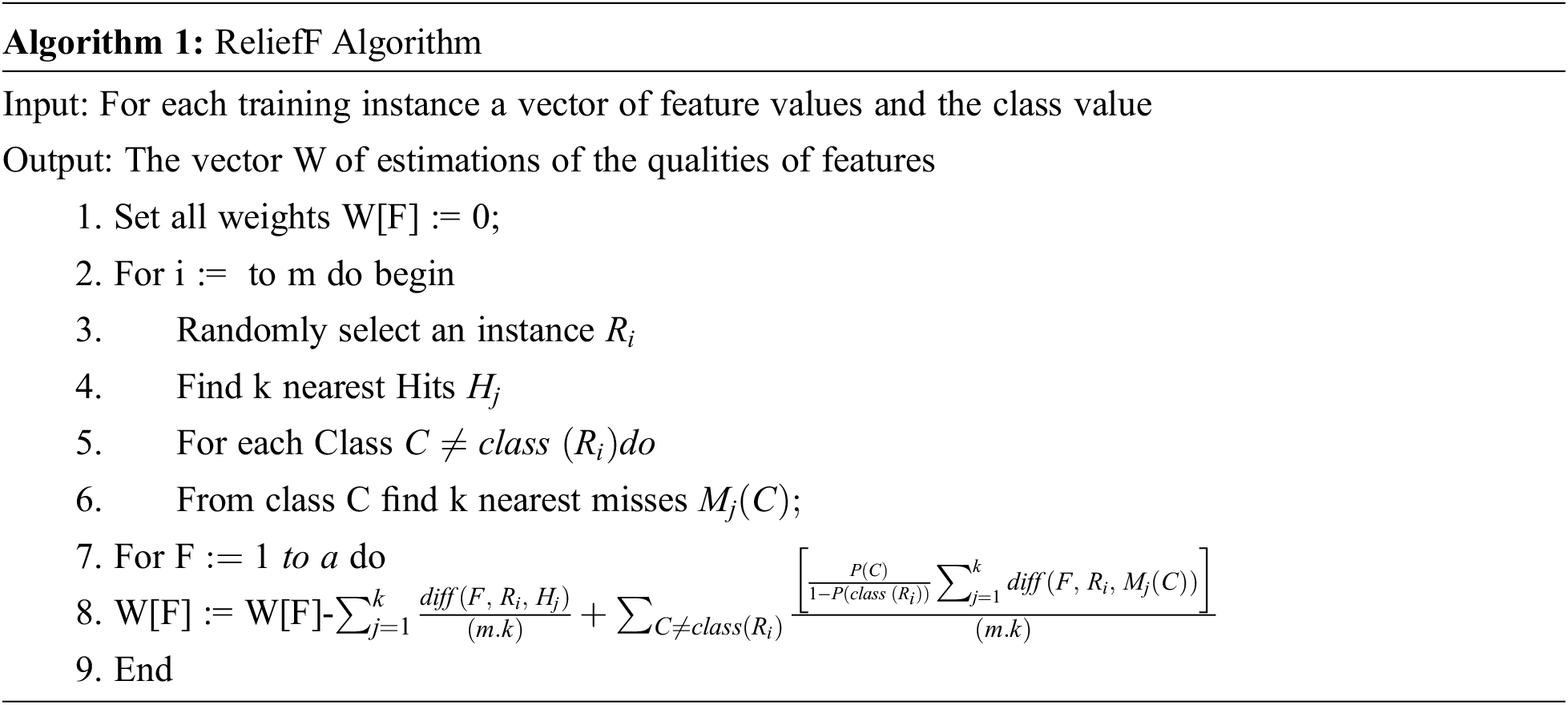
ReliefF differentiates data points that are near to each other in a feature space. A sample drawn instance’s value is compared with instances near to it. A relevance score is then assigned to each feature as good features have a constant value within their class. This process is recursive and features’ scores in iterations are updated. This helps weighing nearest neighbours based on their distance. ReliefF which can handle noisy and incomplete data values is limited to two classes in this work. It randomly selects an instance Ri and searches for k nearest neighbors in the same class (nearest hits Hj ) and different classes (misses Mj(C) . The quality estimation of features F is updated based on Ri , Hj and Mj(C) . Each class’s misses are weighted with the prior probability of that class P(C) Hits and misses are computed in the interval [0,1] where the probability weights total to 1. Misses are divided by probability weight factor 1 − P(class ( Ri )) or sum of probabilities of misses. This process is repeated m times. The selection of user defined k for hits and misses ensures robustness with respect to noises in the data where k controls estimates and is generally set to 10 for safety.

InfoG

InfoG is based on entropy where the weight of each feature is derived by evaluating the extent to which it decreases the class entropy or in reducing class predictions. Entropy can be calculated [25] using Eq. (1):

IG(C, F)=H(C)−H(C|F) (1)

where IG(C, F)-information of feature F in class C, H(C)–class entropy and H (C|F)-conditional class entropy. InfoG is the number of bits saved when the class is transformed. Conditional entropy, depicted in Eqs. (2) and (3) can be computed by splitting the dataset into groups for each observed value of F and the sum of the ratio of examples in the class multiplied by the group’s entropy [25].

H(C|F)=−∑c∈C⁡p(C|F)log⁡p(C|F) (2)

H(C)=−∑c∈C⁡p(C)log⁡p(C) (3)

H(C|F) -conditional class entropy using Eq. (2), H(C) -class entropy using Eq. (3).

GR

GR is also based on entropy, but differs from InfoG in normalizing InfoG’s bias towards greater values. Normalizations are done by dividing InfoG with attribute entropy in a class; as a result it reduces the bias of InfoG algorithm. GR can be computed using Eq. (4) [26].

Gain Ratio (C,F)= (H ©−H (C|F))/H(F) (4)

when features count in a subset increases, difference are more clear and pronounced.

Wrappers

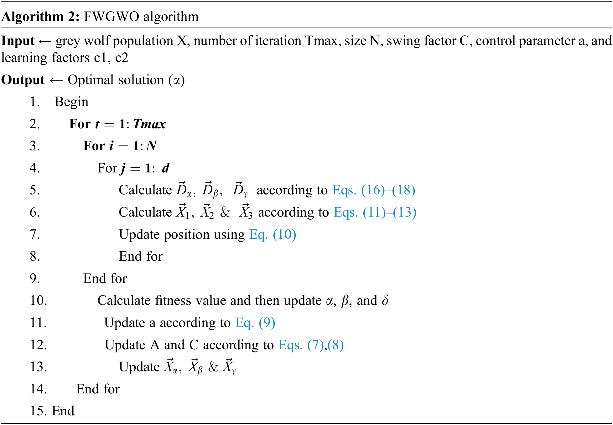
Wrappers use ML for their search of possible feature subsets and evaluate each subset based on quality. This work uses FWGWO (Algorithm 1) with EHO (Algorithm 2) as a wrapper in its operations.

FWGWO

Techniques based on Grey wolves are an advanced implementation of optimizations as they easily close on optimal selection of features (prey) from a dataset. This work uses metaheuristic algorithms which mimic attacking grey wolves for closing in on a prey (optimal selection of features) [27]. Wolves exist in packs of 5–12 and have four levels of leadership hierarchy namely alpha ( α ), beta ( β ), delta ( δ ), and omega ( ω ) as shown in Fig. 2. Alpha represents pack leaders in decision making.

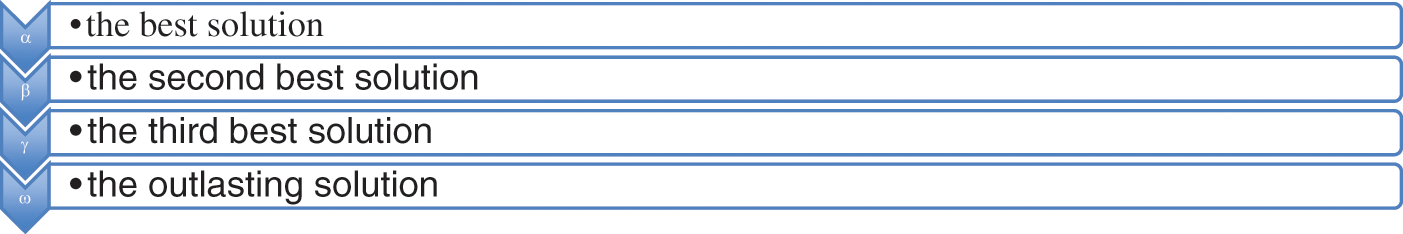
Figure 2: The leadership hierarchy of wolfs

The α , β , and δ are the first, second, third best-recommended optimal features from the dataset in FWGWO algorithm. The best estimated solution in feature elections is ω. In a hunting process, wolves surround their prey in an arrangement that can be depicted mathematically using Eqs. (5) and (6) (5–6) [28]:

D→=|C→. X→P−X→(t)| (5)

X→(t+1)=|X→P(t)−A→.D→| (6)

where X→(t) and X→(p) -locations of grey wolf and prey in iteration (t) for selecting features. The coefficient vectors A→ and C→ in the above equations can be modelled using Eqs. (7) and (8),

A→=|2a→. rand1→−a→| (7)

C→=2. rand2→ (8)

where rand1→ and rand2→ - random vectors in the interval [0,1] in feature selections. a→ is linearly decreased from 2 to 0 by iterations using Eq. (9),

a(t)=as−(as−af)∗(ttmax)2 (9)

where as and af -initial and end value of a control parameter, t–current iteration and Tmax-overall iterations. The iterations parameter controls iterations during feature selection. A grey wolf’s location (X, Y) changes based on its prey position (X∗,Y∗) in selecting features. α , β , and δ mimic hunting behavior for feature selections. Since, three solutions result, remaining wolves change their positions based on three best solutions (X→1,X→2 & X→3) and shown as Eqs. (10)–(13).

X→(t+1)=(X→1.we1+X→2.we2+X→3.we3)3 (10)

X→1=X→α−A→1.(D→α) (11)

X→2=X→β−A→2.(D→β) (12)

X→3=X→δ−A→3.(D→δ) (13)

The weight vector WE=we1(alpha)+we2(beta)+we3(delta) is obtained and its membership function is estimated using interval weights of interval/crisp comparison matrix. If Fw is a fuzzy membership function for a fuzzy set A on the universe of discourse w it is defined as μA: Fw → [0,1], where each element of w is in they interval [0,1], w={we1,we2,we3} and we1≥we2≥we3 . Mathematically, in a search alpha’s weights changes to we1={1.0 to 13} while the weights of the beta and delta change to {0.0 to 13} . y = pimf ( w , params) returns fuzzy membership values computed using a spline-based pi-shaped membership function as depicted in Eq. (14),

Fw=μA(w,a,b,c,d)={0,w≤a2(w−ab−a)2,a≤w≤a+b21−2(w−bb−a)2,a+b2≤w≤c1,b≤w≤c1−2(w−cd−c)2,c≤w≤c+d22(w−dd−c)2,c+d2≤w≤d0,w≥d (14)

Membership values for each weight in w={we1,we2,we3} is computed using Eq. (15).

X→(t+1)=(X→1. Fwe1+X→2. Fwe2+X→3. Fwe3)3 (15)

where, Fwe1,Fwe2,Fwe3 -weights of α , β , and δ .

D→α=|C→1. X→α−X→| (16)

D→β=|C→2. X→β−X→| (17)

D→δ=|C→3. X→δ−X→| (18)

Wolves change their positions for catching a prey where |A| < 1. α , β , and δ wolves pursue the prey and unite on closing. A→1 has takes values > 1 or < −1 randomly.

Proposed Elephant Herding Optimization (EHO)-FWGWO Model

The proposed algorithm for addressing feature selection problems is examined in this section (see Fig. 3). The model is mainly initialized, evaluated, transformed, and iterated.

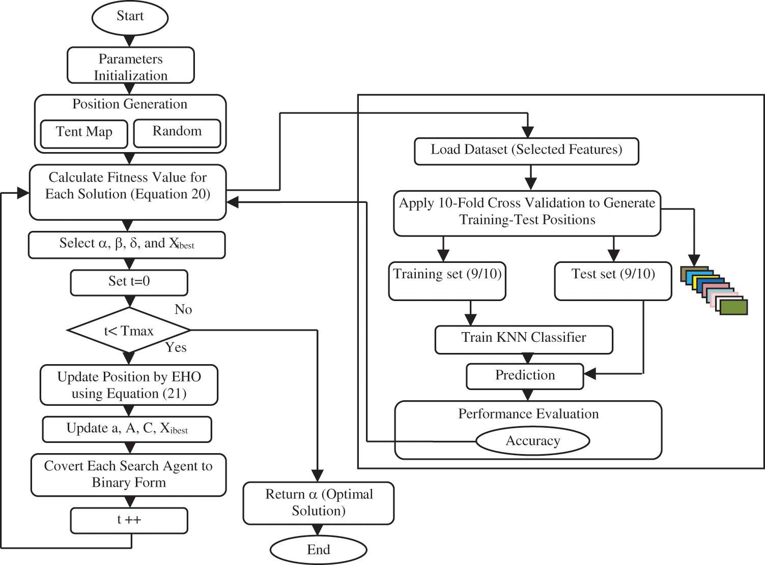
Figure 3: Block diagram for the proposed model

Initialization

In this stage randomly generated n wolves are initialized. These wolves or search agents represent a solution whose length d equates to the features count in the original dataset. Fig. 4 displays a probable dataset solution with 11 features. Relevant features have a value of 1 while ignored features take a value of 0.

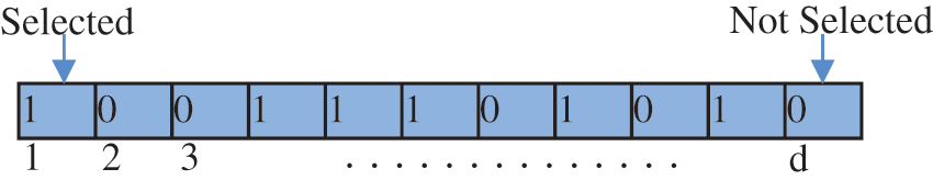
Figure 4: Solution representation

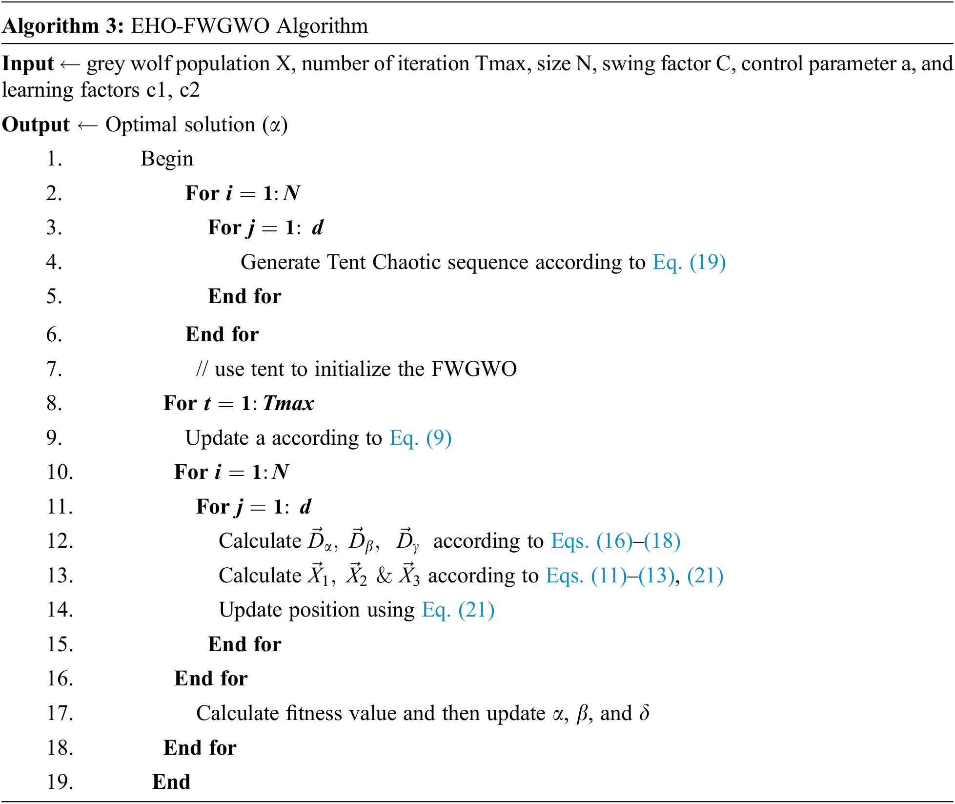
A logistic map generated the initial PSO population where feature convergences in the proposed algorithm rely on random sequences that execute the algorithm using different parameters. The proposed work’s TCM is depicted as Eq. (19).

xk+1={μxkfor0≤xk≤12μ(1−xk)for12≤xk≤1 (19)

where, μ -set to 1+R, R-random value in the range [0,1]. A point x0 in the interval is changed to xk in the range [0,1].

Evaluation

The fitness function used in this work evaluates goals using Eq. (20),

fitness=αγR(D)+β|S||D| (20)

where, γR(D) -present the error rate of KNN, |S| -selected subset feature cardinality (length), |D| -cardinality of all dataset features. α∈[0,1] and β=1−α – weights that reflect accuracy value of classifications and the selected sub-set length.

Position Updating

FWGWO considers the second and third-best locations of wolves for learning location information on specific wolves and in doing so a wolf’s information on own experience is ignored. Hence, the proposed work uses EHO to update positions. FWGWO update are performed based on a clan operator which uses grey wolf’s position in a clan for updates based on the relationship to the operator. EHO methods for updates described by the authors of [29] are used in this study for updating grey wolf positions. Assuming ci denotes a grey wolf clan its subsequent position in the clan is updated using Eq. (21):

Xnew,ci,j(t+1)=c1r2(Fwe1X→1(t)+Fwe2X→2(t)+Fwe3X→3(t))∗Xci,j(t)+a1∗c2r2(Xbest,ci−Xci,j(t))∗r (21)

where, Xnew,ci,j(t) -updated position at iteration t, Xci,j(t) -previous position of grey wolf j in the ci at iteration t. Xbest,ci –fittest wolf in clan ci;, the fittest individual grey wolf. The scaling factor a1∈[0,1] influences matriarch of ci in Xci,j(t) . r∈[0,1] . This is a stochastic distribution which can assess diversity in the population during a search. This work does not use uniform distribution or Xci,j=Xbest,ci implying the fittest grey wolf information cannot be updated using Eq. (21). This is overcome in this work by using EHO for updating individual fittest wolf position given by Eq. (22):

Xnew,ci,j(t+1)=Xcenter,ci(t)×a2 (22)

The issue in the above equation is the absence of a reference source. Hence, information from all individuals in ci is used to create the new best Xnew,ci,j where its centre Xcenter,ci , is calculated for the dth dimension through D (Total Dimensions) calculations using Eq. (23):

Xcenter,ci,d(t+1)=1nci×∑j=1nciXci,j,d(t) (23)

where, 1≤d≤D -dth dimension, nci -count of individuals in ci, and Xci,j,d(t) -dth dimension of the individual Xci,j at iteration t. Based on the feature selection values (0 or 1), most suitable features are chosen for enhancing accuracy of classifiers. The resultant search space is transformed by a sigmoidal function into a continuous binary form [19] using Eqs. (24) to (26),

Xi=xi−MinMax−Min (24)

xsi=11+e−Xi (25)

xbinary={0ifR<xsi1ifR≥xsi (26)

where, xsi -S-shaped search agent’s continuous value (feature), i=1,….,d , and xbinary - values to 0 or 1 using random number R∈[0,1] . Max/Min are maximum/minimum values of the continuous feature vectors. Algorithm 3 lists the EHO-FWGWO algorithms pseudo code.

3.1.2 Embedded Algorithm

This work embeds SVM-t for statistically analyzing features from a dataset for selection as SVMs create a maximal hyper plane from feature vectors to find classes in a dataset. The proposed SVM-t takes advantage of the most significant feature subsets in a dataset using Eq. (27). Two-sample t-statistics in two directions evaluate variances in the determined classes and thus minimizes variations between them for classifying data points into classes.

|tj|=|(uj+−uj−)((sj+)2/n+)+((sj−)2/n−)| (27)

where, n+ (resp., n−)–number of support vectors designed for class + 1 (resp., −1). Compute mean uj+ (resp., uj− ) and standard deviation sj+ (resp., sj− ) by using simply the support vectors of feature j-labelled class + 1 (resp., −1) to calculate the score of every one attribute. The computed features with improved scores represent features that vary in classification. Thus, SVM-t’s perceptive choice of features results in an accurate feature set.

3.2 Aggregation Strategy

Fig. 5 depicts the overall framework of HEFSM in feature selections. HEFSM uses filters, wrappers and embedding for selecting significant features and then orders them based on their importance to produce many sorted optimal feature subsets namely FS1,FS2...FSt . Each feature j in FSi is normalized by using (n-j)/n where n is the total features for computing the feature weight set of the ith feature selection Wgi={wg1i,wg2i...wgni} . The proposed method uses geometric means to compute the total weight of each feature in the set FS1,FS2...FSt , and then sorts features based on the total weight for getting the sorted feature sequence Wg . Geometric mean used in this work is defined as the nth root (n-count of numbers) of the product of the features.

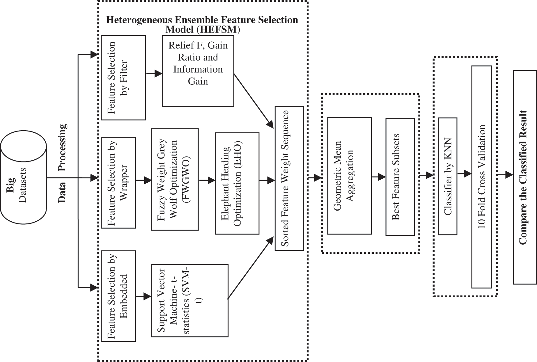
Figure 5: Overall framework of HEFSM method

Geometric mean is obtained by dividing the sum of logarithmic values by the number of features as shown in Eq. (28),

geometric mean= (∏i=1n(FS_i)(1/n))(28)

A threshold percentage th% selects features from this sorted sequences to create an optimal feature subset. All feature selection methods results are joined for forming a single input for the KNN classifier which then validates the proposed scheme’s selected feature sets.

3.3 KNN Classifier

KNN uses Euclidean distances for finding nearest neighbours to data points [30] using Eq. (29).

Eucd(P,Q)=∑i=1d(Qi−Pi)2 (29)

where, Qi and Pi -specific attributes in a sample, i = {1..d}, d – count of used features. One part of the dataset is used for validations while the balance is used for classifications. Since classifiers overfit values, Cross-validation is used to overcome the problem. This work uses a K-fold cross-validation where K = 10 assuming samples are divided into K partitions with similar size in cross validations. KNN is trained with K−1 partitions for predicting labels or classes in the dataset. These classifications are matched against wrong labels for obtaining the classification error percentage. The results obtained from multiple data rounds have been proven to be statistically reliable [31].

4  Results and Discussion

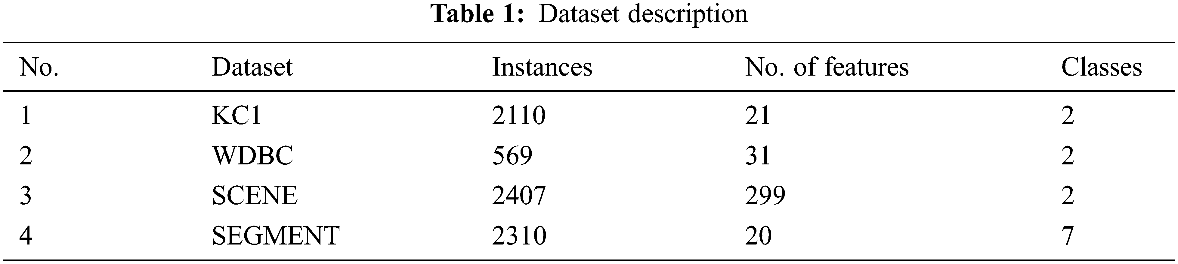
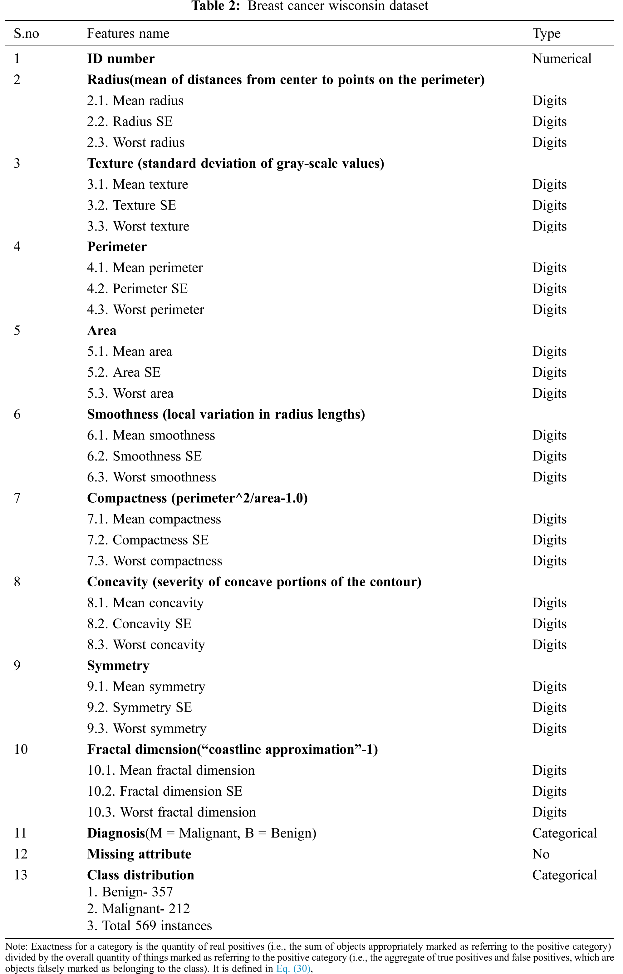
This section displays experimental results of the proposed HEFSM is implemented on MATLAB (2014a) and on an intel core i7/16Gb running 64 bit windows 10. The proposed scheme was examined using known datasets (listed in Tab. 1) with feature selection issues for its ability to select optimal feature sets from datasets. These datasets were obtained from the UCI Machine Learning Repository website [32]–[34]. Breast cancer Wisconsin data collection, characteristics are determined from a digitized representation of a fine needle aspirate (FNA) of a breast mass. They explain the existence of the cell nuclei features that are in the picture. It contains information on the source, donor, clinical studies, id number, diagnosis (malignant = M, Benign = B) and distribution of grades. Ten real-valued functions are determined for each cell nucleus as pursues: radius, texture, perimeter, area, smoothness, compactness, concavity, concave points, symmetry and fractal dimension (See Tab. 1).

All the characteristics are measured for the mean, regular error, and “worst” or highest (mean of the three highest values). 80% of the training data and 20% of the evaluation data are included in the categorization phase for the assigned series of data. Data source of Chronic Kidney Disease (CKD) consist of 400 occurrences with 25 characteristics. This dataset is also used to assess CKD and can be obtained approximately within 8 weeks of time from the hospital (Tab. 2). The scene dataset is an image classification task where labels like Beach, Mountain, Field, and Urban are assigned to each image. Segment instances were drawn randomly from a database of 7 outdoor images. The images were hand-segmented to create a classification for every pixel. Each instance is a 3 × 3 region.

Precision=True Positive(TP) True Positive(TP)+False Positive(FP) (30)

In this case, recall is specified as the quantity of true positives divided by the overall elements truly belonging to the positive class. It is defined in Eq. (31)

Recall=True Positive(TP) True Positive(TP)+False Negative(FN) (31)

F-measure is defined as combination of precision and recall. It is defined in Eq. (32)

F−Measure=2×precision×recallprecision+recall (32)

Classification accuracy is the ratio of correct predictions to total predictions made. It is often described in Eq. (33),

Accuracy =TP+TNTP+TN+FP+FN (33)

The classification accuracy of the KNN classifier conducted in Tab. 3. The resulted accuracies in most datasets approved the superiority of the proposed model. In the scene and segment dataset, the HEFSM achieved better results of 92.85% and 97.23% which is better than other methods. The results in Tab. 3 graphically modelled in the following Figs 6–10. Combining experiments were performed using four feature selection methods and four datasets, shown as 3.

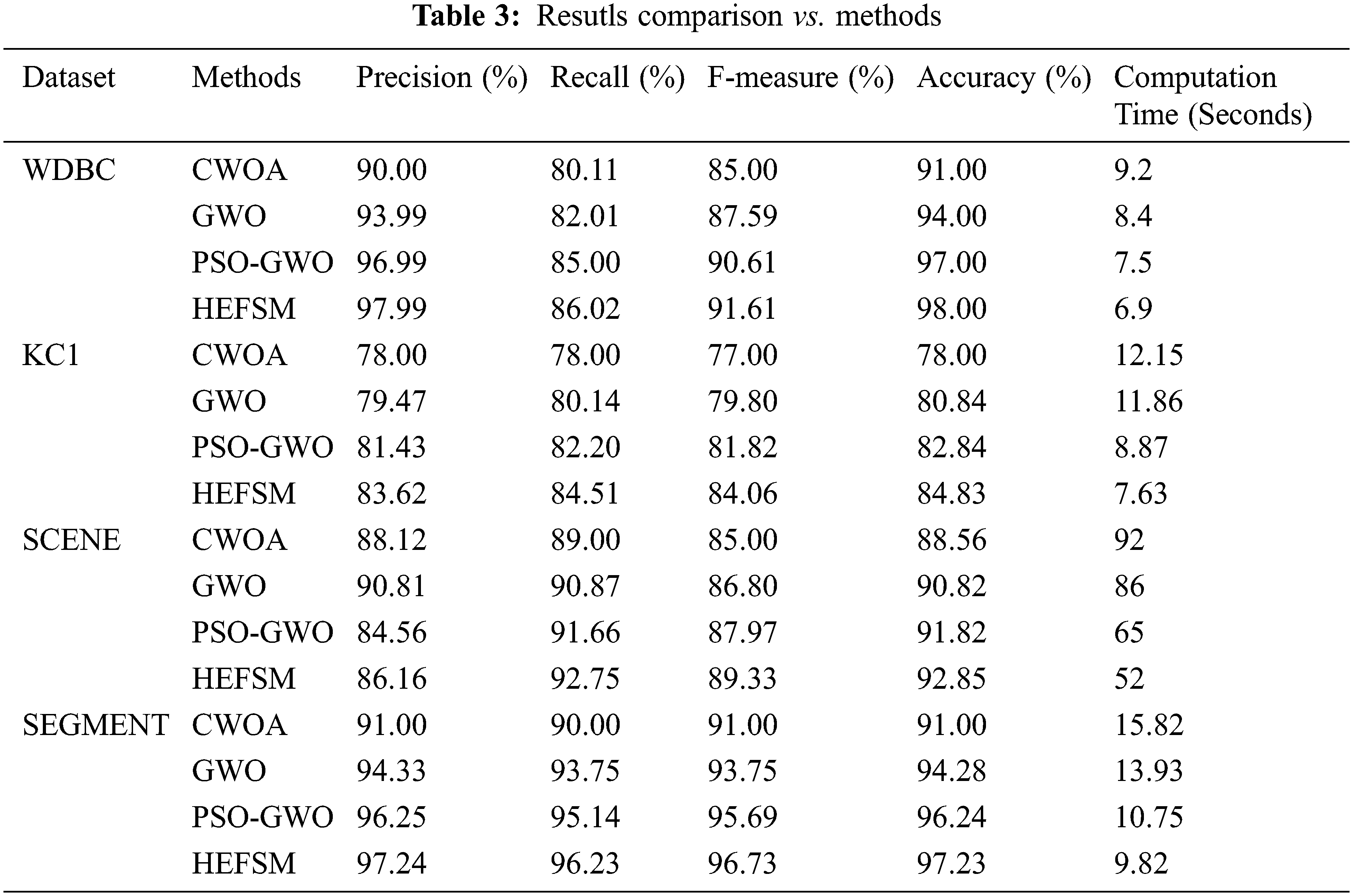
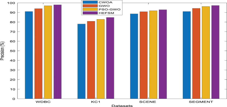
Figure 6: Precision comparison of feature selection methods vs. datasets

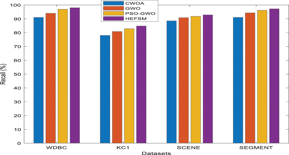
Figure 7: Recall comparison of feature selection methods vs. datasets

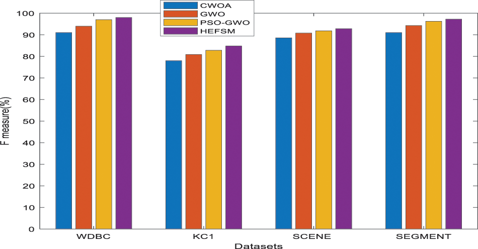
Figure 8: F-Measure comparison of feature selection methods vs. datasets

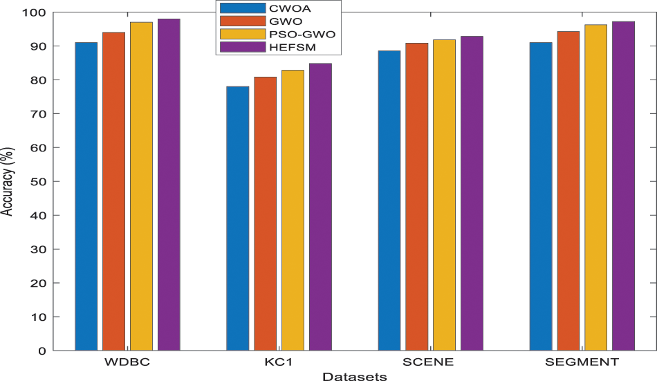
Figure 9: Accuracy comparison of feature selection methods vs. datasets

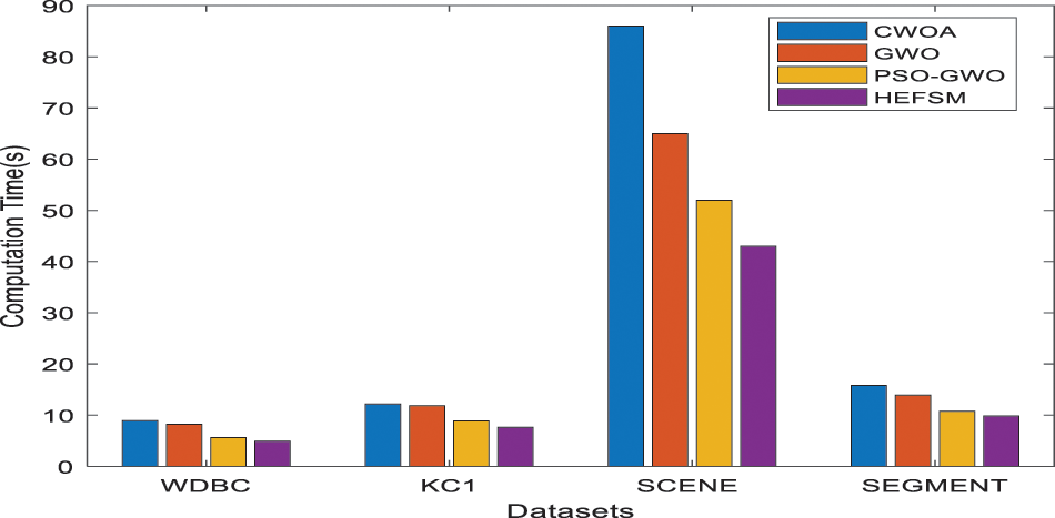
Figure 10: Computational time comparison of feature selection methods vs. datasets

Fig. 6 shows the precision comparison among the proposed HEFSM system and other algorithms concerning the KNN classifier. Fig. 6, the precision result of proposed HEFSM system gives higher results of 97.99% whereas other methods such as CWOA, GWO and PSO-GWO gives lesser precision results of 90.00%, 93.99%, and 96.99% respectively at WDBC dataset. The recall results of feature selection methods are graphically explained in Fig. 7. The proposed model achieved higher recall results of 86.02%, whereas other methods such as CWOA, GWO and PSO-GWO algorithm gives recall result of 80.11%, 82.01% and 85.00% respectively at WDBC dataset concerning the KNN classifier. F-measure results of proposed system and existing feature selection algorithms via KNN classifier are graphically shown in Fig. 8. The proposed model gives improved f-measure results of 91.61%, whereas other methods such as CWOA, GWO and PSO-GWO algorithm gives f-measure result of 85.00%, 87.59% and 90.61% respectively at WDBC dataset concerning the KNN classifier. From the total number of features in all datasets, the proposed HEFSM model via three feature selection methods gives best features which give improved accuracy results. Fig. 9 shows a comparison among the proposed model and other algorithms concerning the accuracy. Tab. 3 shows the accuracy for experiment computations. The results graphically explained in Fig. 9. The proposed model achieved higher accuracy. The accuracy for all datasets has increased when compared to other feature selection methods respectively. Accuracy results of proposed system and existing feature selection algorithms via KNN classifier are graphically shown in Fig. 9. The proposed model gives improved accuracy results of 98.00%, whereas other methods such as CWOA, GWO and PSO-GWO algorithm gives accuracy result of 91.00%, 94.00% and 97.00% respectively at WDBC dataset via KNN classifier. From the total number of features in all datasets, the proposed HEFSM model via three feature selection methods gives best features which give improved accuracy results.

Fig. 10 shows the comparison time among the proposed model and other algorithms concerning the KNN classifier. Tab. 3 shows the elapsed time for experiment computations. The proposed model achieved less computation time of 6.9 s for WDBC dataset. The total time is 9.2 s for CWOA, 8.4 s for GWO and PSO-GWO equals to 7.5 s.

5  Conclusion and Future Work

This paper has proposed and implemented an ensemble learning method HEFSM for selecting optimal feature sets from high dimensional datasets. Multiple techniques and algorithms are used in this proposed work. It uses filters, wrappers and embedding in its architecture. Filtering is based on ReliefF, InfoG and GR. SVM-t is embedded for statistical evaluations and selections. A new binary variant of wrapper functions in feature selection is executed by integrating FWGWO and EHO algorithms for achieving better performances and achieving a better trade-off between predictive performance and stability. The ensemble paradigm has been introduced in the framework for improving robustness of feature selections, specifically for high-dimensional or minimal sampled datasets or data where extracting stable features is complex and difficult. The proposed scheme’s aggregate learning from multiple optimal feature subsets results in higher stability especially while handling high dimensional data in HEFSM. This framework’s EHO-FWGWO algorithm overcomes local optima issues by its random initializations, use of TCM and features weights generated by a fuzzy function. Moreover, the application of a sigmoid function in converting the search space to a binary form increases the proposed systems ability. HEFSM technique could find best feature subsets for maximizing classifier accuracy as proved by the results of KNN classifications on the selected optimal feature subsets. For instance, the proposed model gives improved accuracy results of 98.00%, whereas other methods such as CWOA, GWO and PSO-GWO algorithm gives accuracy result of 91.00%, 94.00% and 97.00% respectively at WDBC dataset via KNN classifier. Invest a significant amount of time in data to increase the model’s reliability and performance. KNN classifier, accuracy depends on the quality of the data and for larger dataset the prediction stage might be slow. In future some other classifiers such Support Vector Machine (SVM), deep learning methods and fuzzy methods have been developed for classification which is left as scope of the future work.

Funding Statement: The authors received no specific funding for this study.

Conflicts of Interest: The authors declare that they have no conflicts of interest to report regarding the present study.

References

1. K. Hi’ovská and P. Koncz, “Application of artificial intelligence and data mining techniques to financial markets,” Economic Studies & Analyses/Acta VSFS, vol. 6, no. 1, pp. 1–15, 2012. [Google Scholar]
2. M. Qiu, S. Y. Kung and Q. Yang, “Secure sustainable green smart computing,” in IEEE Transactions on Sustainable Computing, vol. 4, no. 2, pp. 142–144, 2019. [Google Scholar]
3. B. Johnson, Algorithmic Trading & DMA: An introduction to direct access trading strategies, 1st ed., London: Myeloma Press, pp. 574, 2011. [Google Scholar]
4. J. Cai, J. Luo, S. Wang and S. Yang, “Feature selection in machine learning: A new perspective,” Neuro Computing, vol. 3, pp. 70–79, 2018. [Google Scholar]
5. E. Emary and H. M. Zawbaa, “Feature selection via lèvy antlion optimization,” Pattern Analysis and Applications, vol. 22, no. 3, pp. 857–876, 2018. [Google Scholar]
6. R. C. Chen, C. Dewi, S. W. Huang and R. E. Caraka, “Selecting critical features for data classification based on machine learning methods,” Journal of Big Data, vol. 7, no. 1, pp. 1–26, 2020. [Google Scholar]
7. J. C. Ang, A. Mirzal, H. Haron and H. N. A. Hamed, “Supervised, unsupervised, and semi-supervised feature selection: A review on gene selection,” IEEE/ACM Transactions on Computational Biology and Bioinformatics, vol. 13, no. 5, pp. 971–989, 2015. [Google Scholar]
8. P. Smialowski, D. Frishman and S. Kramer, “Pitfalls of supervised feature selection,” Bioinformatics, vol. 26, no. 3, pp. 440–443, 2010. [Google Scholar]
9. S. H. Huang, “Supervised feature selection: A tutorial,” Artificial Intelligence Research, vol. 4, no. 2, pp. 22–37, 2015. [Google Scholar]
10. N. Hoque, M. Singh and D. K. Bhattacharyya, “EFS-MI: An ensemble feature selection method for classification,” Complex & Intelligent Systems, vol. 4, no. 2, pp. 105–118, 2018. [Google Scholar]
11. M. Sharawi, H. M. Zawbaa and E. Emary, “Feature selection approach based on whale optimization algorithm,” in 2017 Ninth Int. Conf. on Advanced Computational Intelligence (ICACI), Doha, Qatar, pp. 163–168, 2017. [Google Scholar]
12. G. I. Sayed, A. Darwish and A. E. Hassanien, “A new chaotic whale optimization algorithm for features selection,” Journal of Classification, vol. 35, no. 2, pp. 300–344, 2018. [Google Scholar]
13. K. Chen, F. Y. Zhou and X. F. Yuan, “Hybrid particle swarm optimization with spiral-shaped mechanism for feature selection,” Expert Systems with Applications, vol. 128, pp. 140–156, 2019. [Google Scholar]
14. S. Gu, R. Cheng and Y. Jin, “Feature selection for high-dimensional classification using a competitive swarm optimizer,” Soft Computing, vol. 22, no. 3, pp. 811–822, 2018. [Google Scholar]
15. Q. Tu, X. Chen and X. Liu, “Hierarchy strengthened grey wolf optimizer for numerical optimization and feature selection,” IEEE Access, vol. 7, pp. 78012–78028, 2019. [Google Scholar]
16. F. Haiz, A. Swain, N. Patel and C. Naik, “A Two-dimensional (2-D) learning framework for particle swarm based feature selection,” Pattern Reorganization, vol. 76, pp. 416–433, 2018. [Google Scholar]
17. H. M. Zawbaa, E. Emary, C. Grosan and V. Snasel, “Large-dimensionality small-instance set feature selection: A hybrid bio-inspired heuristic approach,’’ Swarm Evolution Computer, vol. 42, pp. 29–42, 2018. [Google Scholar]
18. S. Fong, R. Wong and A. Vasilakos, “Accelerated PSO swarm search feature selection for data stream mining big data,” IEEE Transaction. Services Computer, vol. 9, no. 1, pp. 33–45, 2016. [Google Scholar]
19. M. Abdel-Basset, D. El-Shahat, I. El-henawy, V. H. C. de Albuquerque and S. Mirjalili, “A new fusion of grey wolf optimizer algorithm with a two-phase mutation for feature selection,” Expert Systems with Applications, vol. 139, pp. 1–14, 2020. [Google Scholar]
20. Q. Li, H. Chen, H. Huang, X. Zhao, Z. Cai et al., “An enhanced grey wolf optimization based feature selection wrapped kernel extreme learning machine for medical diagnosis,” Computer Mathematics Methods, vol. 2017, pp. 1–15, 2017. [Google Scholar]
21. I. M. El-Hasnony, S. I. Barakat, M. Elhoseny and R. R. Mostafa, “Improved feature selection model for big data analytics,” IEEE Access, vol. 8, pp. 66989–67004, 2018. [Google Scholar]
22. J. Wang, J. Xu, C. Zhao, Y. Peng and H. Wang, “An ensemble feature selection method for high-dimensional data based on sort aggregation,” Systems Science & Control Engineering, vol. 7, no. 2, pp. 32–39, 2019. [Google Scholar]
23. B. Pes, “Ensemble feature selection for high-dimensional data: A stability analysis across multiple domains,” Neural Computing and Applications, vol. 32, pp. 1–23, 2019. [Google Scholar]
24. I. H. Witten, E. Frank, M. A. Hall and C. J. Pal, Data Mining: Practical Machine Learning Tools and Techniques, Burlington: Morgan Kaufmann, vol. 2, pp. 1–664, 2016. [Google Scholar]
25. I. Kavakiotis, O. Tsave, A. Salifoglou, N. Maglaveras, I. Vlahavas et al., “Machine learning and data mining methods in diabetes research,” Computational and Structural Biotechnology Journal, vol. 15, pp. 104–116, 2017. [Google Scholar]
26. H. Dağ, K. E. Sayin, I. Yenidoğan, S. Albayrak and C. Acar, “Comparison of feature selection algorithms for medical data,” in 2012 Int. Symp. on Innovations in Intelligent Systems and Applications, Karadeniz Technical University, pp. 1–5, 2012. [Google Scholar]
27. S. Mirjalili, S. M. Mirjalili and A. Lewis, “Grey wolf optimizer,” Advances in Engineering Software, vol. 69, pp. 46–61, 2014. [Google Scholar]
28. Z. J. Teng, J. L. Jv and L. W. Guo, “An improved hybrid grey wolf optimization algorithm,” Soft Computing, vol. 23, no. 15, pp. 6617–6631, 2019. [Google Scholar]
29. G. G. Wang, S. Deb and L. D. S. Coelho, “Elephant herding optimization,” in 2015 3rd Int. Symp. on Computational and Business Intelligence (ISCBI), Indonesia, pp. 1–5, 2015. [Google Scholar]
30. J. Gou, H. Ma, W. Ou, S. Zeng, Y. Rao et al. “A generalized mean distance-based k-nearest neighbor classifier,’’ Expert System Applied, vol. 115, pp. 356–372, 2019. [Google Scholar]
31. T. T. Wong and P. Y. Yeh, “Reliable accuracy estimates from k-fold cross validation,” IEEE Transtions Knowledge Data Engineerng, Early Access, vol. 2, pp. 635–651, 2019. [Google Scholar]
32. E. D. Dheeru and K. Taniskidou, “UCI machine learning repository,” Technical Representation, vol. 5, pp. 586–592, 2017. [Google Scholar]
33. W. Sun, X. Chen, X. R. Zhang, G. Z. Dai, P. S. Chang et al., “A Multi-feature learning model with enhanced local attention for vehicle re-identification,” Computers, Materials & Continuous, vol. 69, no. 3, pp. 3549–3560, 2021. [Google Scholar]
34. W. Sun, G. C. Zhang, X. R. Zhang, X. Zhang and N. N. Ge, “Fine-grained vehicle type classification using lightweight convolutional neural network with feature optimization and joint learning strategy,” Multimedia Tools and Applications, vol. 80, no. 20, pp. 30803–30816, 2021. [Google Scholar]
Cite This Article
Copyright © 2023 The Author(s). Published by Tech Science Press.
This work is licensed under a Creative Commons Attribution 4.0 International License , which permits unrestricted use, distribution, and reproduction in any medium, provided the original work is properly cited.
Downloads
Citation Tools