Profiling of Urban Noise Using Artificial Intelligence

1  Introduction

Pollution in general is a pressing global issue. In addition to environmental, air or light pollution, noise pollution is gaining attention as it significantly affects quality of life for humans. It has been proven that exposure to noise pollution can lead to health issues such as stress, high blood pressure, heart disease, sleep disruption, hearing loss and even learning and cognitive impairment in children [1], not to mention the impacts on the economy [2], and society or the major disruption on ecosystems [3–5]. Out of all the types of environmental pollution, noise pollution receives the least awareness, possibly a contributing factor as to why exposure to noise pollution has exceeded safety limits in many countries [6]. The impact of noise pollution affects everyone alike, irrespective of wealth or income levels. The World Health Organization claims that exposure to sound levels of 70 dB or less, even for a lifetime, will not cause any health issues [7]. However, short-term exposure to loud noise is inevitable, and limits for children and adults differ. For children, the peak sound pressure that they are exposed to must not exceed 120 dB. For adults, the limit for sound pressure levels is 140 dB. Some sources causing noise pollution are traffic, public address systems, railways or neighborhoods. In areas where there is indiscriminate use of vehicle horns or loudspeakers, people could face health hazards such as headaches, deafness or nervous breakdow [8]. With exposure to noise above 75 dB, for more than 8 h a day for long periods of time, hearing impairment can occur. When exposed to a bursting cracker, tinnitus will occur and possibly even permanent hearing loss. Another hazard of noise pollution is causing sleep disturbances, especially when noises cause awakening in early morning hours and results in difficulty falling asleep again [9]. With the identification and classification of noise, solutions can be identified to eliminate noise pollution and elevate quality of life. Noise management is essential for improving air quality, transport planning, urban planning and green area planning, by targeting noise pollution. As traffic is one of the most significant contributors to noise pollution, the European Commission [10] proposes to establish quiet areas within a city and develop cost-effective plans to reduce noise. By limiting or controlling volumes of traffic in an urban area, there will be a direct impact on improving noise pollution. Profiling of urban noise using AI is a way to help further research on noise reduction that focuses specifically on cities and urban areas, as accurate classification leads to efficient reduction.

2  Related Works

Prevention of noise pollution is possible, and one method is by reducing noise emissions. Asmussen et al. [11] investigated reducing noise emission from railways by increasing damping, which has been shown to reduce vibration of energy and reduce noise generated by tracks. The results of their investigation showed a reduction in noise of up to 4 dB from increased damping, and future improvements in the size and spacing of the dampers could further reduce noise. Instead of reducing noise, Renterghem [12] conducted a study on creating insulation against noise using green roofs. It was found that using green roofs were able to reduce sounds heard near or inside a building by 20 to 30 dB compared to 10 to 20 dB of non-vegetated insulation roofs. This is due to the high surface mass density, low stiffness, and damping properties of green roofs, making them an effective insulator for sound transmission. Halim et al. [13] investigated other forms of noise barriers as a prevention method using hollow concrete blocks and panel concrete. They concluded that hollow concrete blocks were able to reduce noise transmission by up to 9.4 dB and that this insulation remained stable for 1 month.

Previously, a traditional method of classifying noise was using the Gaussian mixture model (GMM), as Ozerov et al. [14] have done in their study by using it to recognize who said the last sentence in a conversation. An advantage of using GMM, especially when trained using clean data, is that some models are able to cope with missing data from nonstationary distortions when features are sometimes masked. However, collecting clean data is difficult; For example, indexing television requires recognizing when each speaker is speaking, and recording in a controlled environment is not always possible. Ma et al. [15] on the other hand, used the hidden Markov model (HMM) to classify noise in urban environments. Their investigation showed that HMM is efficiently modeled when sound is produced from a single point source, resulting in an accuracy of 100% in 3 of 10 tests. But in an environment where mixtures of noises exist, HMM has difficulty being modeled as some components are not stationary and have no constraint on the form of sounds which results in the classifier not recognizing noises.

Artificial intelligence (AI) is extremely versatile and capable of making decisions independently of humans through algorithms and functions that allow AI to discriminate and label various sensory input. Utilizing neural networks, deep learning and Markov models, the application of AI in sound classification is impactful. Classification with neural networks operates by extracting information in the form of feature vectors. A problem arises with sound due to information being mixed together, creating difficulty for classification. Anagnostopoulos et al. [16] have also discovered that classification of sound in real life situations will challenge neural networks as people sometimes speak in short bursts and make non-linguistic sounds (um, ah). Among AI approaches to sound classification, deep learning is widely preferred due to its ability to handle large amounts of data, usually showing better performance compared to neutral networks, according to the review by Lecun et al. [17]. This technique utilizes brute-force training, however, which doesn’t always result in accuracy because of overfitting. Cisse et al. [18] have demonstrated the inaccuracy of deep learning in a study of fooling deep learning models using adversarial input, where the inputted phrases are nonsense but sound similar to legitimate phrases. Markov models, specifically HMM, are one of the most notable AI systems used for sound classification. It benefits sound classification by having a time series probability distribution, resulting in efficient modeling as each word cues the next word likely to appear. Ikhsan et al. [19] has tested HMM in the classification of digital music genres and obtained a maximum accuracy of 80% for 40 amounts of data of each genre. This value is a significant increase from a similar study by Brendan [20] using neural networks that resulted in a maximum accuracy of 67%. Various research has been carried out with the aim to classify sound and improve urban noise pollution, many of which take advantage of AI for efficiency. Bai et al. [21] mapped the distribution of noise with urban sound tagging (UST) to identify whether noise pollution is audible or not, leading to optimization of technology monitoring noise pollution. A convolutional neural network (CNN) based system for UST was utilized so that urban sound could be detected with spatio-temporal context and make use of the capability of feature extraction, but the model had difficulty identifying some sounds due to distractors present. Davis. [22] experimented with environmental sound classification using CNNs along with various data augmentation methods. As data augmentation allows the quality of training data to increase, the accuracy of the system was higher. The study concluded the highest accuracy of 83.5% by using the time stretch augmentation dataset. When testing urban sound classification with CNNs compared to long short-term memory (LSTM), Das et al. [23] discovered LSTM shows better results than CNN for many features used. Zhou et al. [24] also used CNN to classify environmental sound, although with a focus on the network input issue which few studies have investigated. Their experiment results reveal that input does have an effect on classification performance, with the best performance achieved with moderate time resolution input spectrograms. Salamon et al. [25] proposed a new approach to deep CNN, using audio data augmentation to overcome data scarcity, for environmental sound. These augmentation methods will be applied to training data with the purpose of making the network become invariant to deformations and generalize better data.

From the previous studies mentioned, researchers intend to improve machine learning models or input data enhancement, or both, to reach the highest classification accuracy. The training data used are key to achieving high accuracy. Data input must be of high quality, requiring data augmentation and removal of distractors to be performed on training data. Although most studies use CNN, we will use LSTM since this system yields better results. Furthermore, self-attention layers will be included to minimize the total computational complexity. An advanced machine learning technique, the self-attention LSTM method, was applied to our urban sound-noise profiling problem. As proposed by Wang et al. [26], an attention mechanism that can capture the key part of a sentence in response to a given aspect will be designed. This has proven to be beneficial, improving performance compared with several baselines. The method is practical as we only need to process important parts of the data and can ignore the rest, making it applicable when gathering information with long-term dependencies. We plan to train our deep learning model with the Urbansound8k dataset to make our classification diverse and specific without sacrificing accuracy. Data augmentation techniques such as time shift and random noise with extraction methods such as mel frequency cepstral coefficients MFCC, mel-spectrogram will be combined for testing on our proposed training model.

3  Methods

3.1 Schematic Design

The overall structure of our proposed profiling urban sound system is given in Fig. 1. It consists of serial models such as data augmentations, spectrograms’ specialty extractions mechanism, and LSTM layers.

Figure 1: Proposed schematic system

Sound from noise sources in cities are standardized and transformed into the mono format with the sample rate of 22050 Hz. Noise sources will then be extracted into two types of acoustic feature, mel-spectrogram and MFCC from each recording. For the sake of our approach, we have used two LSTM layers. The LSTM model is inductive bias, therefore missing functions to help the model actually learn related things to the input. This leads to errors that tend to occur to long inputs such as vanishing gradients, not compatible with structural data. By adding self-attention layers to the hidden state stage, we have created a vector representing each time interval. In this way, the representing vector can grasp important details over time. These hidden vectors will be connected to the hidden state stage and will be considered in the input as abstract information. Finally, fully connected layers are utilized to learn this abstract information, and softmax regression is used to find the probability distribution of the output.

3.2 Dataset Preparation

Our chosen dataset for training is the Urbansound8k dataset [27]. This dataset is composed of 8732 labeled sound excerpts, each with a duration of four seconds or less. The sounds are divided into 10 profiles that include air conditioning, car horn, children playing, dog bark, drilling, engine idling, gunshot, jack hammer, siren, and street music.

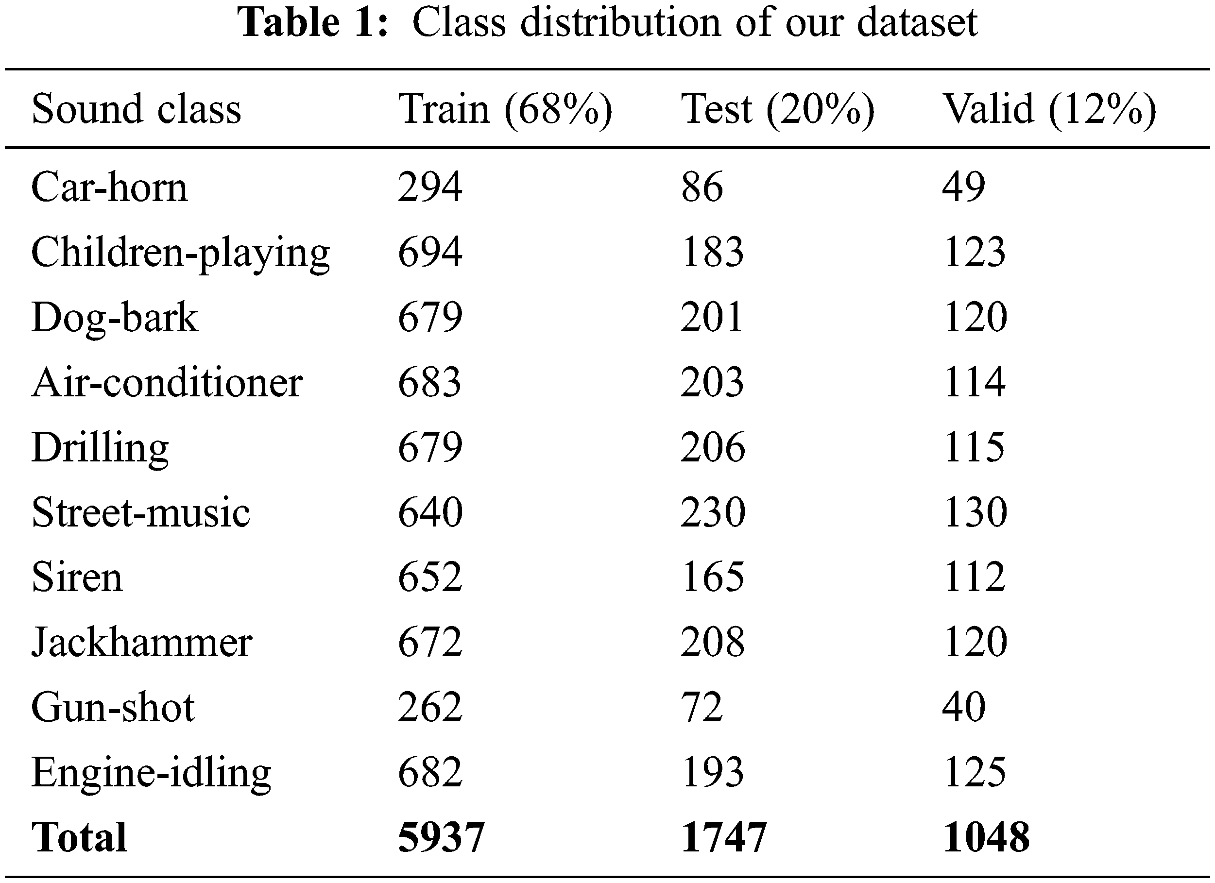
The sounds from this dataset specifically pertain to urban environments, making it ideal for our aim of profiling urban noise. To generate new samples and overcome the problem of imbalanced data and dataset scarcity, we applied different data augmentation methods to extend the data available. Several data augmentation methods are used to alter the sounds and generate variety such as time shifting which moves the time of the audio profile forward or backwards randomly within 230–1360 milliseconds and adds random noise with randomized data from 0 to 0.5%. The results after augmenting the data have been divided into 3 parts: 68% training, 12% valid, and 20% test. Tab. 1 represents the results collected.

3.3 Audio Spectral Feature Extraction

In our profiling investigation, we have used spectral features where we converted audio that has gone through data augmentation from time domain to frequency domain using Fourier transformations. Two different features investigated using the deep architectures are mel-spectrograms and MFCC [28] features, as they provide distinguishable information and representations that are effective in classifying audio signals more accurately. Mel-spectrogram is one of the more popular features used for sound classification due to its suitable characteristics. It can provide the training model with sound information similar to what humans can hear. This means that the spectrogram also mimics our ability to differentiate lower frequencies more easily than higher frequencies.

Extracting features from audio signals is made easier with the help of the Torchaudio [29] library where built-in Python functions exist to generate the required spectrograms. The features collected from the mel-spectrogram or MFCC are the loaded audio and the sample rate of audio at a default of 22050 Hz, which are then processed by Torchaudio’s functions. The function returns 128 mel-spectrogram and 40 MFCC. Using the “car-horn” sound as a particular data sample and extracting the spectrogram, we obtained Fig. 2 presented according to mel-spectrogram and Fig. 3 is presented according to MFCC.

Figure 2: Mel-spectrogram of car horn

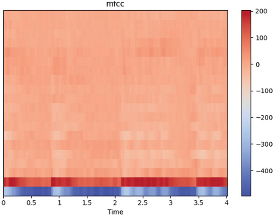
Figure 3: MFCC of car horn

3.4 Model Architecture

3.4.1 Long Short-Term Memory

LSTM is a network capable of remote dependent learning, first introduced by Hochreiter & Schmidhuber in 1997, then improved and applied in many fields such as: robot control, time series prediction, speech recognition, and time series anomaly detection. Fig. 4 illustrates the architecture of a standard LSTM. In Fig. 4, there is supplementing cell internal state st and the three gates for cells including forget gate ft , input gate it , and output gate ot . At each time step t , every gate receives input values xt representing a cell in the input and the ht−1 value from the output of the memory cell from previous time steps t−1 .

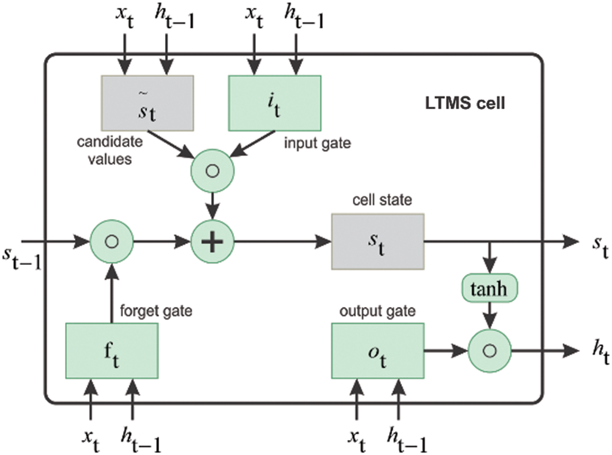
Figure 4: Architecture of a standard LSTM cell

Each gates have their separate and specific goal:

Forget gate: removes unnecessary information before they reach the cell internal state

Input gate: selects necessary information to add to the cell internal state

Output gate: identifies information from the cell internal state to be considered as output information

Regularly each cell in LSTM will be represented by the formulas below:

ft=σ(Wf,xxt+Wf,hht−1+bf) (1)

st~=tanh(Ws~,xxt+Ws~,hht−1+bs~) (2)

it=tanh(Wi,xxt+Wi,hht−1+bi) (3)

st=ft⨀st−1+it⨀st~ (4)

ot=σ(Wo,xxt+Wo,hht−1+bo) (5)

ht=ot⨀tanh(st) (6)

where xt is the input vector at each time step t , Wf,x , Wf,h , Ws~,x , Ws~,h , Wi,x , Wi,h , Wo,x , Wo,h are the weighted matrices and bf,bs~,bi,bo are biases of LSTM to be learned during training. ft,it,ot each contains activation values for the input, forget and output gates respectively. σ is the sigmoid function and ⨀ stands for element-wise multiplication. st,s~ each contains vectors representing cell internal state and candidate value, and ht is a vector of the hidden layer. We regard the last hidden vector hN as the representation of sound noise and put hN into a softmax layer after linearizing it into a vector whose length is equal to the number of class labels. However, the standard LSTM cannot detect which is the important section for aspect-level classification. In order to address this issue, we propose to design an attention mechanism that can capture the key part of an audio in response to a given aspect.

3.4.2 Self-Attention with LSTM

Attention functions will be used, where a query and a set of key-value pairs will be mapped to an output. The vectors are the query, keys, values, and outputs. Computing the weighted sum of the values will result in the output and the weight assigned to each value will be found from computations of the compatibility functions of the query with the corresponding key. The self-attention mechanism, also known as the scaled dot-product attention mechanism described in the study [30], is shown in Fig. 5.

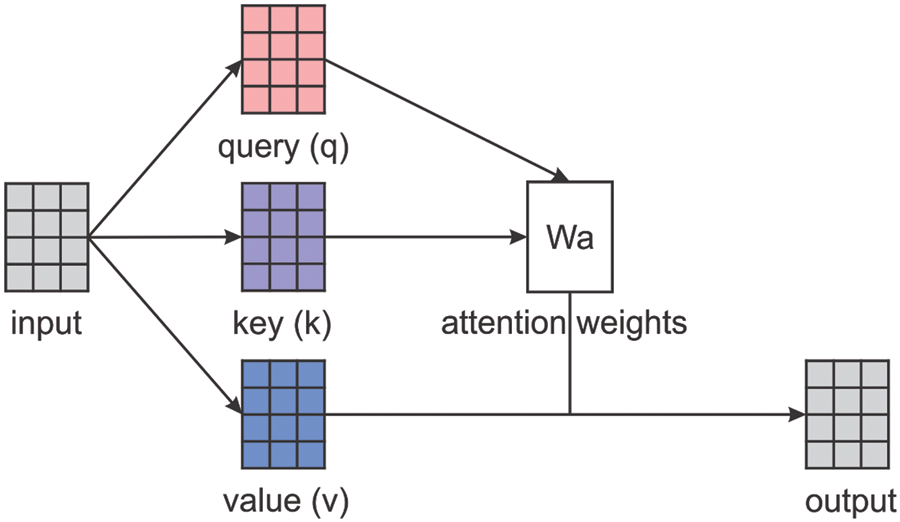
Figure 5: Scaled dot-product attention system

In the figure mentioned above, the input passes through the query q and the key k following dk . We have calculated the cross product of queries and keys, divided it by the root square of d , and softmax was applied to get the weight between [0−1] , then the output would be equal to the product of the same weight above and the value v . So, q,k and v vectors are actually neural networks, therefore if they have the same input as q(x),k(x) and v(x) then they are self-attending. With our input as h[1,2,…,N] , the self-attention expression is written as:

a(h)=attention(h)=softmax(q(h).k(h)dk(h))v(h) (7)

By adding the 2 vectors ( hn and Waa(h) ) to create a new h∗ vector:

h∗=concat(hn,Waa(h)) (8)

where, h∗ are projection parameters which carry information from the hidden state and attention to be learned during training. Wa is the weight to convert a(h) into vectors, with hn as the hidden state at their final status.

The attention mechanism allows the model to capture the most important part of an audio data series when different aspects are considered. A softmax layer is immediately followed after that to transform h∗ into conditional probability distribution.

y=softmax(Wsh∗+bs) (9)

where Ws and bs are the parameters for the softmax layer.

4  Results and Discussion

We used Google Colab as our training environment along with Python and the Pytorch library. The NVIDIA Tesla P100 PCie 3.0 was also used with 16 GB of RAM and 12 GB of RAM (Random Access Memory) on the CPU (Central Processing Unit). We did the training in 50 epochs and in the process, we saved all checkpoints where the valid loss is the highest. At the end of the training process, we loaded every checkpoint and predicted the outcome of the data collected from training. Our research process led us to identify mel-spectrogram and MFCC as inputs that would produce the highest accuracy. Results gathered show the mel-spectrogram as the feature that achieved higher accuracy in both LSTM and self attention LSTM models. Although MFCC is a widely used feature in sound classification, in our study mel-spectrogram yields better results by a small margin. This could be due to the fact that urban sounds are being classified and MFCC is less accurate because its representation is very compressible, likely to be more decorrelated as well. From interpreting results of training loss and accuracy, mel-spectrogram is the better input.

4.1 Loss Function

The sample datasets were randomly divided into the training set, validation set and test set with ratios as shown in Tab. 1. Using these samples, the identification model is trained and verified. Dividing the dataset into several batches helped speed up the training process. Based on the memory of the workstation, the batch size was set to 50. Random initialization was used to initialize the model parameters. The number of training epochs is set to 100. The difference between the spans of collected vocalization signals caused the number of spectrograms for each urban noise in the sample set to differ. Hence, we introduced the weighted cross-entropy as the loss function of the model. The problem of having unbalanced data can then be solved as the loss function can increase the weight of the urban sound noises with few samples. Fig. 6 shows the loss of function during training, we see the self attention LSTM models overall experience a decrease in loss over epoch faster than LSTM models. The reduction in training loss is interpreted as our model having improved accuracy. In each epoch, data is passed forward and backward. Although our training models had up to 100 epochs, training loss stops improving at around 90 epochs for all models. Therefore, an ideal model should have about 95 epochs. The results above suggest this is a suitable stopping point as using more epochs may cause overfitting to occur because the model is memorizing the data given. Large amounts of repetition will allow our model to work effectively with the training data chosen, but will not function well for other datasets.

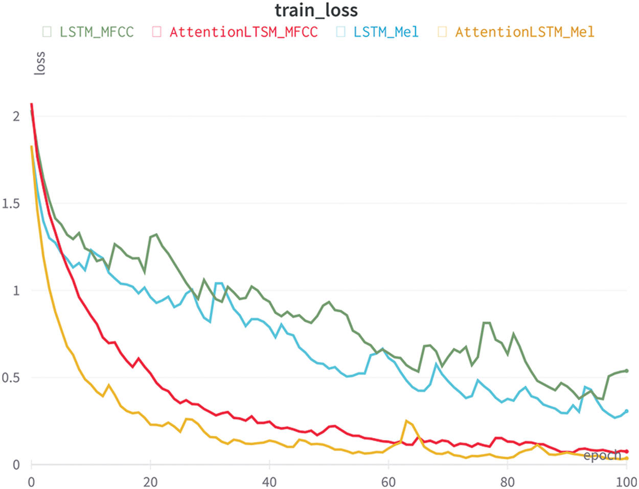
Figure 6: Training loss with various models

4.2 Performance of Metric

The metric we will be using in both of our models is an accuracy metric which is the fraction of our model’s predictions. It represents the validation data accuracy of the model during training and is calculated by taking the number of correct predictions divided by the number of total predictions.

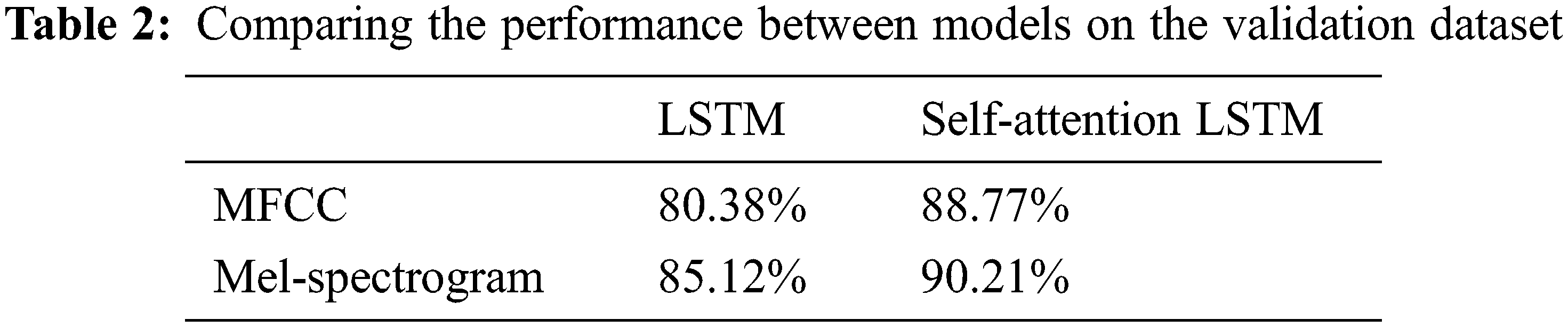
Our model’s training accuracy is portrayed in Fig. 7. An increasing trend in accuracy for all four models is shown as the epoch increases from 0 to 100, which is reasonable as the data are reviewed more times. With the self-attention LSTM models, it takes about 60 epochs, a relatively short time, for convergence. Training beyond this will likely result in overfitting. At certain points the values from the MFCC input may result in higher accuracy but in general the mel-spectrogram input yields better results. As predicted, the self-attention LSTM models with mel-spectrogram and MFCC result in higher and stabilized accuracy compared to LSTM models. The steep initial increase in accuracy of the LSTM functions is due to the effectiveness of self-attention. The weakness of LSTM models is the inability to detect important parts for aspect-level classification. This leads to low convergence, and the accuracy reached is not at a sufficient level for the classification model to be used. Such results support our reasoning of including self-attention in the training model. After training, checking with the validation dataset allowed us to compare the accuracy of the process as shown in Tab. 2. The highest accuracy is 90.21%, achieved by the self-attention LSTM model with mel-spectrogram input. The difference between the accuracy of the LSTM model with MFCC input and self-attention LSTM with mel-spectrogram is rather significant. It can be reasoned that the choice of using a self-attention model capable of identifying relevant information combined with the less compressible mel-spectrogram input was a sound decision to improve accuracy.

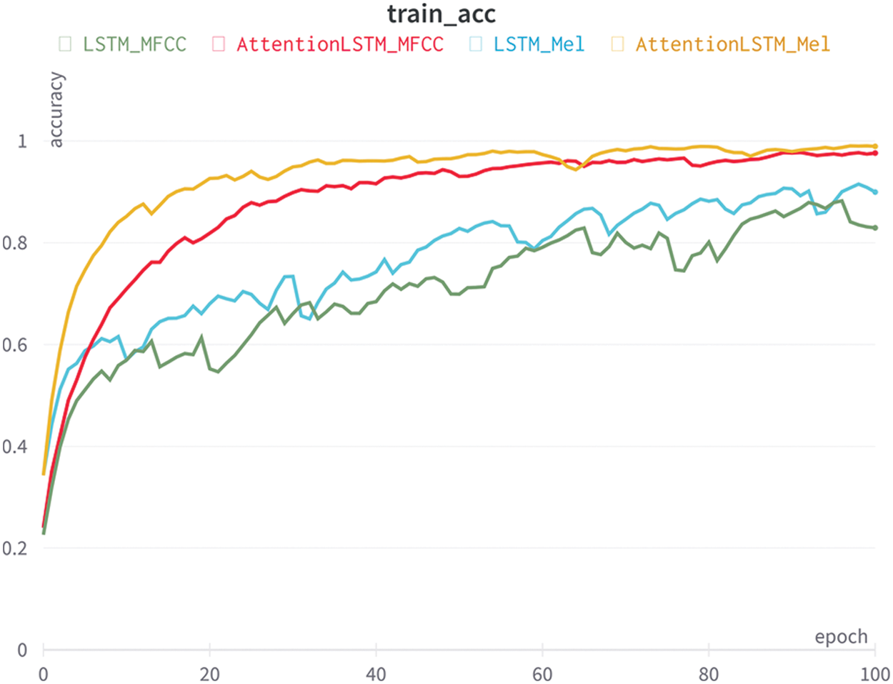
Figure 7: Training accuracy with various models

4.3 Fusion System

We have demonstrated the confusion matrix of our best performing approach which is self-attention LSTM using stacked features of mel-spectrogram. Since it outperformed all the previous models, we declare our approach as the best solution for urban sound noise classification.

The confusion matrix reported for this case in Fig. 8 shows that the architecture is successful in modeling even though some sounds are identical, the percentage of profiling them accurately is very high. An example of this is the “children-playing” class and the “street-music” class. Our model still classified them at a very high accuracy of 83%. The result indicates that with our model, classifying almost identical sounds is possible, with a rather high accuracy rate. With the jackhammer class, our model was able to predict and classify it with an accuracy of up to 98%, likely because this noise source is different and difficult to be confused with other common noises in an urban environment. The reliability of the results found is supported by the large amount of training data, data augmentations, and data specifications.

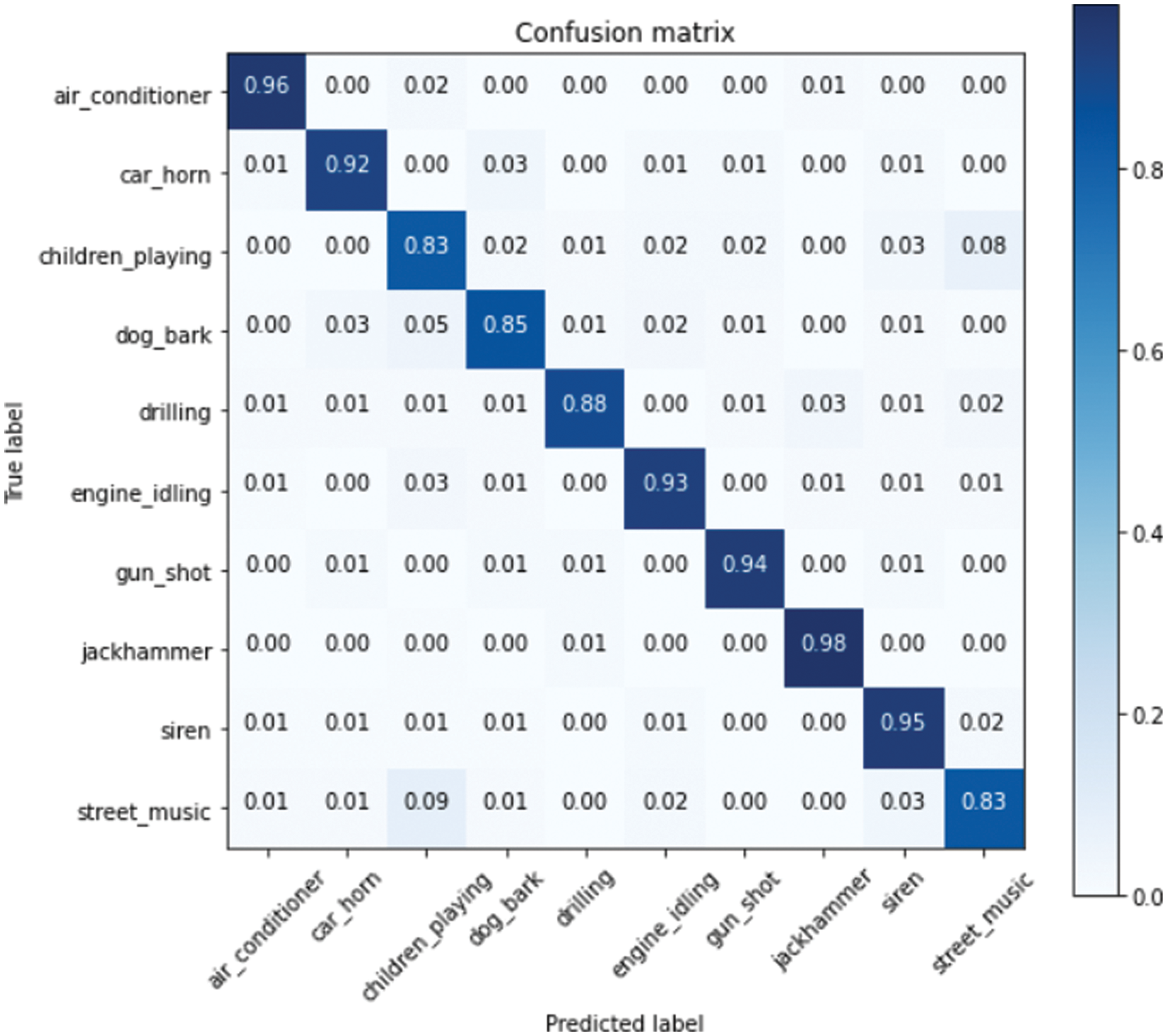
Figure 8: Confusion matrix of our system

5  Conclusions

While mentioned works when using CNN to classify environmental sound sources of the UrbanSound8k dataset to ultimately classify urban noises achieve results like 91% [31] and 93% [32], We on the other hand presented an approach to sound classification and proposed the use of a machine reading simulator to address the limitations of recurrent neural networks when processing inherently structured input. Our model is based on a LTSM architecture embedded with a memory network, explicitly storing contextual representations of input tokens without recursively compressing them. More importantly, a self-attention mechanism is employed for memory addressing, as a way to induce undirected relations among tokens. The attention layer is not optimized with a direct supervision signal, but with the entire network in downstream tasks. Both models have been trained and tested with the original UrbanSound8K and its augmented dataset. Various features are tested such as mel-spectrogram and MFCCs in combination with the architectures to reveal the best feature architecture combination. The result of the fusion multi-channel modes has gained excellent performance profiling urban sound noise, we recommend that researchers choose self-attention for profiling sound problems and if possible, even for problems that involve highly complex sound.

Many different tests and experiments have been left for the future due to time constraints. This problem is caused by the process of gathering real data in the open world. This act is very time-consuming, taking days to gather enough sound to be classified. Our future work will go deeper into the analysis of a particular mechanism, applying our system to different sound classes or we will even apply sound classification on an embedded system for noise recognition purposes. From there we can evaluate the need for clear spaces in cities to reduce noise.

Author’s Contributions: The authors read and approved the final manuscript.

Availability of Data and Materials:All data and materials will be available upon request.

The datasets analyzed during the current study are available in the UrbanSound8K repository, https://www.kaggle.com/chrisfilo/urbansound8k.

Code for training during the current study are available in the LSTM-Attention repository, https://github.com/cuong3004/LSTMAttention.

Funding Statement: The authors received no specific funding for this study.

Conflicts of Interest: The authors declare that they have no conflicts of interest to report regarding the present study.

References

1. S. A. Stansfeld and M. P. Matheson, “Noise pollution: Non-auditory effects on health,” British Medical Bulletin, vol. 68, no. 1, pp. 243–257, 2003. [Google Scholar]
2. Socio-economic impact, accessed May, 2007. Available: http://www.noiseineu.eu/en/14-socioeconomic_impact. [Google Scholar]
3. N. Koper, L. Leston, T. M. Baker, C. Curry and P. Rosa, “Effects of ambient noise on detectability and localization of avian songs and tones by observers in grasslands,” Ecology and Evolution, vol. 6, no. 1, pp. 245–255, 2015. [Google Scholar]
4. L. Jacobsen, H. Baktoft, N. Jepsen, K. Aarestrup, S. Berg et al., “Effect of boat noise and angling on lake fish behaviour,” Journal of Fish Biology, vol. 84, no. 6, pp. 1768–1780, 2014. [Google Scholar]
5. Y. Samuel, S. J. Morreale, C. W. Clark, C. H. Greene and M. E. Richmond, “Underwater, low-frequency noise in a coastal sea turtle habitat,” The Journal of the Acoustical Society of America, vol. 117, no. 3, pp. 1465–1472, 2005. [Google Scholar]
6. A. Ghosh, K. Kumari, S. Kumar, M. Saha, S. Nandi et al., “Noiseprobe: Assessing the dynamics of urban noise pollution through participatory sensing,” in Proc. of the 2019 11th Int. Conf. on Communication Systems & Networks (COMSNETS), Bengaluru, India, pp. 451–453, 2019. [Google Scholar]
7. Berglund, Birgitta, Lindvall, Thomas, Schwelaet al, “Guidelines for community noise,” World Health Organization, 1999, Available: https://apps.who.int/iris/handle/10665/66217. [Google Scholar]
8. N. Singh and S. C. Davar, “Noise pollution-sources, effects and control,” Journal of Human Ecology, vol. 16, no. 3, pp. 181–187, 2017. [Google Scholar]
9. A. Muzet, “The need for a specific noise measurement for population exposed to aircraft noise during night-time,” Noise & Health, vol. 4, no. 15, pp. 61–64, 2002. [Google Scholar]
10. Cities and urban development, accessed Jan, 2017. Available: https://ec.europa.eu/. [Google Scholar]
11. B. Asmussen, D. Stiebel, P. Kitson, D. Farrington and D. Benton, “Reducing the noise emission by increasing the damping of the rail: Results of a field test,” in Noise and Vibration Mitigation for Rail Transportation Systems. Notes on Numerical Fluid Mechanics and Multidisciplinary Design, B. Schulte-Werning (ed.Berlin, Heidelberg, Springer, Vol. 99, pp. 229–230, 2008. [Google Scholar]
12. T. V. Renterghem, “Green roofs for acoustic insulation and noise reduction,” Nature Based Strategies for Urban and Building Sustainability, section III, chapter 3.8, pp. 167–179, 2018. [Google Scholar]
13. H. Halim, R. Abdullah, A. A. A. Ali and J. Mohd, “Effectiveness of existing noise barriers: Comparison between vegetation, concrete hollow block, and panel concrete,” Procedia Environmental Sciences, vol. 30, pp. 217–221, 2015. [Google Scholar]
14. A. Ozerov, M. Lagrange and E. Vincent, “GMM-based classification from noisy features,” in Int. Workshop on Machine Listening in Multisource Environments, Florence, Italy, pp. 6, 2011. [Google Scholar]
15. L. Ma, D. J. Smith and B. P. Milner, “Context awareness using environmental noise classification,” in 8th European Conf. on Speech Communication and Technology, Geneva, Switzerland, pp. 4, 2003. [Google Scholar]
16. C. N. Anagnostopoulos, T. Iliou and I. Giannoukos, “Features and classifiers for emotion recognition from speech: A survey from 2000 to 2011,” Artificial Intelligence Review, vol. 43, no. 2, pp. 155–177, 2015. [Google Scholar]
17. Y. LeCun, Y. Bengio and G. Hinton, “Deep learning,” Nature, vol. 521, no. 7553, pp. 436–444, 2015. [Google Scholar]
18. M. Cisse, Y. Adi, N. Neverova and J. Keshet, “Houdini: Fooling deep structured prediction models,” Arxiv, vol. abs/1707.05373, pp. 12, 2017, https://doi.org/10.48550/arXiv.1707.05373. [Google Scholar]
19. I. Ikhsan, L. Novamizanti and I. N. A. Ramatryana, “Automatic musical genre classification of audio using hidden markov model,” in 2nd Int. Conf. on Information and Communication Technology, Bandung, Indonesia, pp. 397–402, 2014. [Google Scholar]
20. P. Brendan, “Music genre classification using a backpropagation neural network,” In: Labrosa, pp. 2, 2010, https://www.brendanpetty.com/projects/music-genre-classification-project/musicgenreclassification-report.pdf. [Google Scholar]
21. J. Bai, J. Chen, M. Wang and X. Zhang, “Convolutional neural networks based system for urban sound tagging with spatiotemporal context,” Arxiv, vol. 2011.00175, pp. 11, 2020, https://doi.org/10.48550/arXiv.2011.00175. [Google Scholar]
22. N. Davis and K. Suresh, “Environmental sound classification using deep convolutional neural networks and data augmentation,” IEEE Recent Advances in Intelligent Computational Systems, pp. 41–45, 2018. [Google Scholar]
23. J. K. Das, A. Ghosh, A. K. Pal, S. Dutta and A. Chakrabarty, “Urban sound classification using convolutional neural network and long short term memory based on multiple features,” in Fourth Int. Conf. on Intelligent Computing in Data Sciences, Fez, Morocco, pp. 1–9, 2020. [Google Scholar]
24. H. Zhou, Y. Song and H. Shu, “Using deep convolutional neural network to classify urban sounds,” in IEEE Region 10 Conf., vol. 10, pp. 3089–3092, 2017. [Google Scholar]
25. J. Salamon, C. Jacoby and J. P. Bello, “A dataset and taxonomy for urban sound research,” in Proc. of the 22nd ACM Int. Conf. on Multimedia, Orlando, Florida, USA, pp. 1041–1044, 2014. [Google Scholar]
26. Y. Wang, M. Huang, X. Zhu and L. Zhao, “Attention-based LSTM for aspect-level sentiment classification,” in Proc. of the 2016 Conf. on Empirical Methods in Natural Language Processing, Austin, Texas, USA, pp. 606–615, 2016. [Google Scholar]
27. Urbansound8K, accessed Jan, 2014. Available: https://urbansounddataset.weebly.com/urbansound8k.html. [Google Scholar]
28. M. Huzaifah, “Comparison of time-frequency representations for environmental sound classification using convolutional neural networks,” ArXiv, vol. abs/1706.07156, pp. 5, 2017, https://doi.org/10.48550/arXiv.1706.07156. [Google Scholar]
29. Torchaudio document, accessed Jan, 2021. Available: https://pytorch.org/audio/stable/index.html. [Google Scholar]
30. A. Vaswani, N. Shazeer, N. Parmar, J. Uszkoreit, L. Jones et al., “Attention is all you need,” ArXiv, vol. abs/1706.03762, pp. 15, 2017, https://doi.org/10.48550/arXiv.1706.03762. [Google Scholar]
31. M. Massoudi, S. Verma and R. Jain, “Urban sound classification using CNN,” in 6th Int. Conf. on Inventive Computation Technologies, Coimbatore, India, pp. 1–8, 2021. [Google Scholar]
32. W. Mu, B. Yin, X. Huang, J. Xu and Z. Du, “Environmental sound classification using temporal-frequency attention based convolutional neural network,” Scientific Reports, vol. 11, no. 1, pp. 25, 2021. [Google Scholar]
Cite This Article
Copyright © 2023 The Author(s). Published by Tech Science Press.
This work is licensed under a Creative Commons Attribution 4.0 International License , which permits unrestricted use, distribution, and reproduction in any medium, provided the original work is properly cited.
Downloads
Citation Tools