Signal Conducting System with Effective Optimization Using Deep Learning for Schizophrenia Classification

1  Introduction

Schizophrenia (SZ) is a harmful and prolonged brain disorder which affects normal speech, thinking, and the behavioral characteristics of a person. These days widely almost 1% of people affected mental disorder as per the report of World Health Organization (WHO) and the impact of this affect the people life. The symptoms of them are hallucination, disorganized discourse, and delusions [1]. Because of the problems in some brain functions [2], schizophrenia easily happens and people in different sectors have been caused by this disease [3,4]. To an individual, this disease cause damage in a micro-level and to the country this disease has affected a big cause in macro-level which affects the country economic system also. The person with symptoms of psychotic disorder shows impacts in their daily routine [5].

Therefore, the diagnosing of schizophrenic patients is becoming the serious topic. EEG is a low-cost and an effective device to record the activity of the brain [6,7]. Now-a-days, EEG has been largely exploited in the diagnosis of several nervous system diseases like Alzheimer’s disease, epilepsy, and schizophrenia. EEG can be implemented by placing the electrodes on Schizophrenia patient’s scalp at different location [8]. Based on the analysis, the existing technique is required to provide effective outcomes in terms of effective diagnosing and cognitive analysis with low resolution.

EEG provides detailed information about the disease by analyzing the characteristics of the signal transformation [9]. Therefore, EEG is considered as an efficient tool for predicting neurological disorders [10]. The EEG measurement setup shown in Fig. 1 is based on 64 channels. Several schizophrenia based analysis are processed which includes classification and interpretation based on neurological disorder [11]. This can be done through the utilization of machine learning (ML) and Deep Learning (DL) techniques.

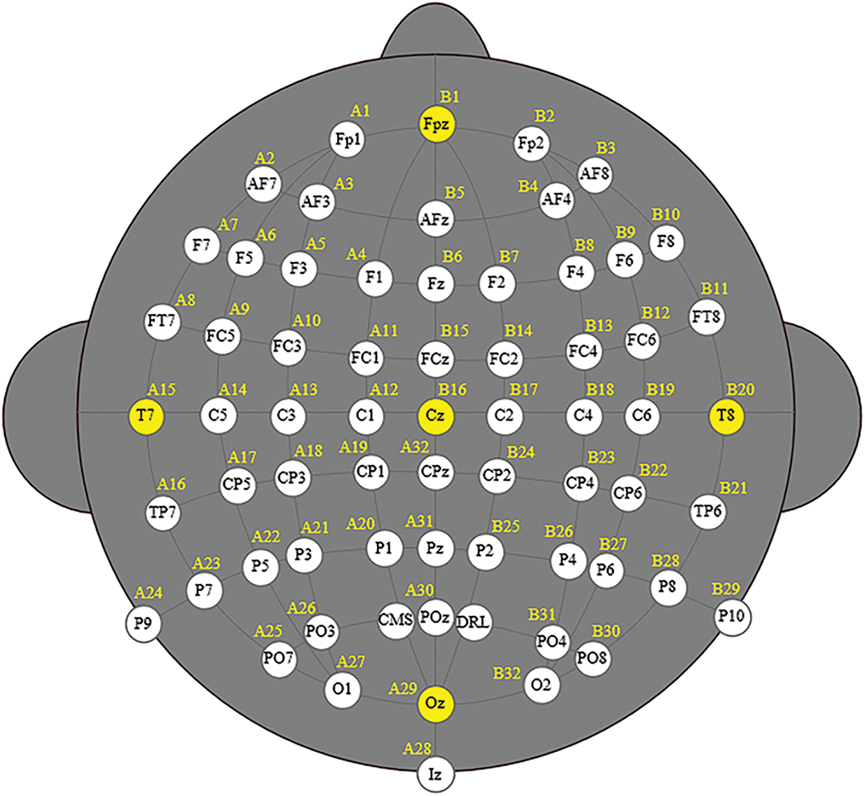
Figure 1: Illustrates the EEG 64 channels

ML algorithms have been used for SZ classification which is primarily based on traditional classifiers such as Decision Tree (DT), Linear Discriminant analysis (LD), K-Nearest Neighbor (KNN) and kernel discriminant analysis (KDA) [12,13]. These methods require large datasets for processing. In the applications of neuroscience, the advancement of DL shows the promising results, therefore, the DCNN is used as proposed methodology for this research work.

The major contributions of the works are:

•   19-channel EEG signals are utilized for both schizophrenia class and normal pattern.

•   Then 157 features from each EEG patterns are utilized based on Non-linear feature extraction process.

•   To improve the efficiency of the system DCNN with mayfly optimization algorithm is used.

•   Finally, the system performance is analyzed by comparing the proposed method over the conventional methods.

2  Problem Statement

This section specifies the existing problems in EEG based signal conduction system for predicting the Schizophrenia detection.

•   All the brain monitoring functions may fail to provide detailed information about the diseased portion; therefore, there is a requirement to utilize the EEG modality which is highly recommended. Moreover, cost is also affordable for diagnosing disease. So there is a necessity to enable an effective technique for enhancing the performance of the EEG based diagnosing modality with high spatio-temporal resolution data.

•   Schizophrenia classification relies on effective feature extraction based on EEG signals. The existing techniques are not as much as effective. Therefore, the Machine Learning (ML) based feature extraction can be considered as an alternative for effective feature extraction.

•   The existing technique [14], is not fully working with large datasets; therefore, the utilization of a large dataset for developing an effective signal conducting system based on EEG signal are highly demanded for Schizophrenia early prediction.

•   The detection and classification based on EEG signal is not effective with existing techniques. To enhance it further we need to use an appropriate Deep Learning technique.

3  Literature Review

This section focuses on literature review related to signal conducting with EEG data for Schizophrenia disease prediction. For this analysis, the articles from 2016 to 2021 are collected and analyzed in terms of techniques used.

In 2020, Prabhakar et al. proposed four feature extraction methods such as Isometric Mapping, non-linear regression technique, partial least squares and expectation maximization based principal component analysis for classifying the SZ from EEG signals. Then, optimization algorithms were used for this feature optimization. Then the classification was done with the help of the Adaboost classifier and Naïve Bayesian Classifier. The implemented method showed its efficiency with a classification accuracy of 98.77%.

In 2019, Oh et al. [14] have presented a technique for SZ detection using a convolutional neural system. Here, the model collected the EEG signals from 28 people, where they were equally for healthy as well as SZ patients and created CNN model with 11 layers for verifying the signals. During the convolution stage, the features were extracted and the fully connected layer was used for classification. This model provides 98.07% of accuracy for healthy patient and 81.26% of accuracy for SZ patients.

In 2020, Sharma et al. [15] have developed schizophrenia detection by EEG signals with features of statistical and non-statistical. From a set of 16 electrodes, variance, higuchi fractal dimension, correlation and mean were calculated for these electrodes. Analysis was taken from each electrode to find a potential electrode set. From the features, SZ detection has been carried out by potential electrodes. Here the classification was done by Support Vector Machines (SVM) classifier and the results showed that SVM achieved a 100% of accuracy.

In 2019, Phang et al. [16] have proposed a DCNN for EEG classification to detect SZ. The features were hybrid by using CNN with multi-domain connection that contained one-dimensional and two-dimensional CNNs. An apparent group between healthy patient and SZ were identified by learning the representation of hierarchical latent from EEG signals [17]. When comparing with single-domain CNN, this model with combined connectivity achieved 93.06% of accuracy with the fusion of decision-level.

In 2016 Santos-Mayo et al. [18] used the wave of P3b and designed a Computer-aided diagnosis (CAD) system to identify the healthy and SZ. CAD system consists of EEG preprocessing [19,20], feature extraction, grouping of 7 electrodes, discriminant feature selection, and binary classification. Finally, the proposed method was compared over different ML classification methods [21] on the basis of certain measures.

In 2020 Sunil Kumar Prabhakar et al. [22] used four features such as lempel ziv complexity, detrend fluctuation analysis, largest lyapunov exponent and recurrence quantification analysis to classify the EEG signal for SZ. The results showed that a classification accuracy of 92.17% is obtained when Black-Hole (BH) optimization is utilized with SVM-Radial Basis Function (RBF) kernel.

Rumelhart et al. [23] defined Error back propagation (BP) as the popular algorithm for training DNNs. DNNs is a powerful technique for combining and generating information from multimodal data. CNN has demonstrated better performance in many computer vision tasks [24]. Hence, the CNN models are promising in processing clinical diagnosis and expression data to detect mental health conditions.

In 2021 Fu et al. [25] designed a novel Sch-net neural network based on a CNN, which perform the SZ speech detection using DL techniques. The proposed Sch-net combines the advantages of the two components, which can avoid the procedure of manual feature extraction and selection.

According to 10–20 international standards, horizontal and vertical eye movements of patients are recorded and extracted the EEG signals from 21 gold cup electrodes, where these were studied in Kim et al. [26].

In 2021 Zülfikar et al. [27] detect the SZ disease using the features of time frequency and Visual Geometry Group-16, a pre-trained model of CNN is used for training process and key features are extracted from scalogram images.

In 2015, Aharon et al. [28] presented the “TFFO” (Time-Frequency transformation followed by Feature-Optimization), a novel approach for SZ detection. The recordings for single node are suitable for this approach and process of data acquisition is feasible for the quick detection of SZ.

In 2020, Zulfikar et al. [29] revealed that there is a relationship between frequency components of an EEG recording and the SZ disease. In 2019, Torres Naira et al. [30] represented the relations between channels by using Pearson correlation coefficient and used the shorter matrix as an input to the CNN.

From the analysis of the several research articles, the existing techniques utilized for SZ disease are analyzed and understood for developing the novel EEG based diagnosing framework.

4  Proposed Methodology

4.1 Data Acquisition

During the data acquisition phase, the proposed model is based on obtaining the dataset from the open source internet “https://www.kaggle.com/broach/buttontonesz2”. This helps to obtain better results with a proposed model.

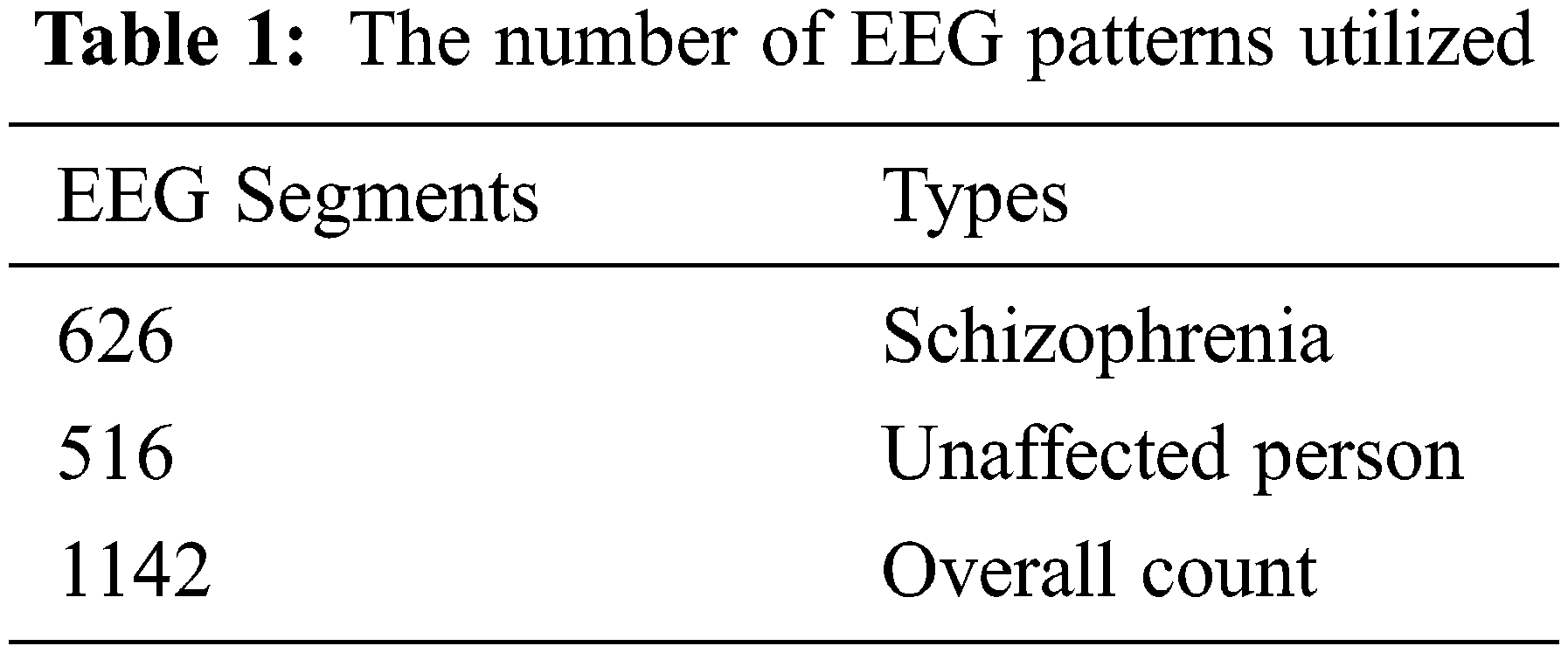
The dataset is adopted with 14 subjects as normal and 14 as affected schizophrenia disease from the Institute of Psychiatry and Neurology based on Poland. This is inclusive of 7 males with average age of 27.0 + 3.3 years and the number of females is 7 with average age of 28.3 + 4.1 years. For this dataset collection, the patients are in the state of relax with closed eye position. In this process, within 15 min of time period, the obtained EEG signals are in 19 channel. Each channel is associated with 2, 25,000 samples that can be partitioned into 5000 groups as sample segments. This is based on the formation of [5000 * 45] as the data matrix of each channel. In Tab. 1, the two classes based EEG segments are provided.

For the implementation of this work, the proposed work is made up of 19 electrodes including C3, C4, Cz, F4,F2, F1, F7, F3, T5, T4, Pz, T5, Pz, P3, P4, O1, O2, and T6. Therefore, this is considered as the multi-channel EEG signal.

4.2 Pre-Processing and Feature Extraction

The overall architecture of the proposed model is shown in Fig. 2. In the pre-processing stage, EEG signals based feature extraction is done by Particle Swarm Optimization (PSO). Therefore, the signals are segmented as non-overlapping of 25 s. This is done by considering 6250 × 19 sample points. The segmentation carried out as 1142 EEG patterns, then the collected signals to form a new database in terms of schizophrenia and normal patients with fixed length. Then, the feature extraction is processed by means 157 non-linear features from EEG classes. From the 157 features based Student’s t-test, the selection process is done based on 14 features by means of optimal features. The employed features are KolmogorovSinai entropy (k-s), Rényi(re), Tsallis(ts), largest Lyapunov exponent(lx), permutation entropy(pe), Shannon(sn), Hjorth complexity(hc), mobility(hm), cumulant(c), bispectrum (bs), cumulant(c), and Kolmogorov complexity(kc).

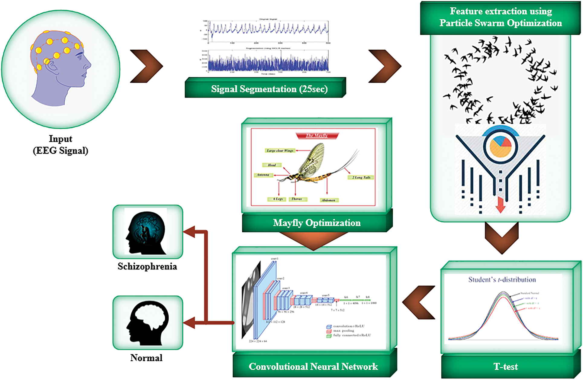
Figure 2: Overall architecture of the proposed model

4.3 Classification

Several existing techniques are used for classifying two classes (affected or not-affected) based on image as well as signal based classification. The widely used algorithms are Decision Tree (DT), Linear Discriminant (LD), K-Nearest Neighbors (KNN), etc., DT based classifier is processed based on tree-like configuration with a sequence of test sequences. LD classifier executes based on matching category by analyzing the combination of values. This work is based on DL based classification process; therefore, DCNN is considered as most suitable technique for classifying the diseases. The DCNN is improved by utilizing the May Fly optimization technique that provides enhancement in the model. This enhances the performance and efficiency of the proposed technique.

The architecture of Deep CNN is complex due to its parameters and masked layers. It is mainly associated with three tiers such as convolution, fully connected, and max pooling. In this process, the kernels with different sizes are utilized for signal processing and it is taken as input during training protocol. In the convolutional operation, feature extraction process is executed from input signals. Then the extracted features are transferred to next layer. The batch normalization process is executed for normalizing the training data in the middle layers. Therefore, the learning process can be enhanced for further processing. In the max pooling layer, the feature map’s size can be changed, this provides high number of kernels. The output obtained from the convolutional and pooling layers depicts the essential features of the input data. Based on the prior results, the fully connected layer executes the categorization process by considering input data to form different classes. In this architecture, the neurons are interconnected in max pooling and fully-connected; therefore, the expected outcome can be predicted as normal or not as shown in Fig. 3. This work highly relies on better performance and efficiency. The CNN is improved by adopting the Mayfly optimization for enhancing the performance. The combination of CNN and Mayfly algorithm may produce good results in terms of performance analysis methods.

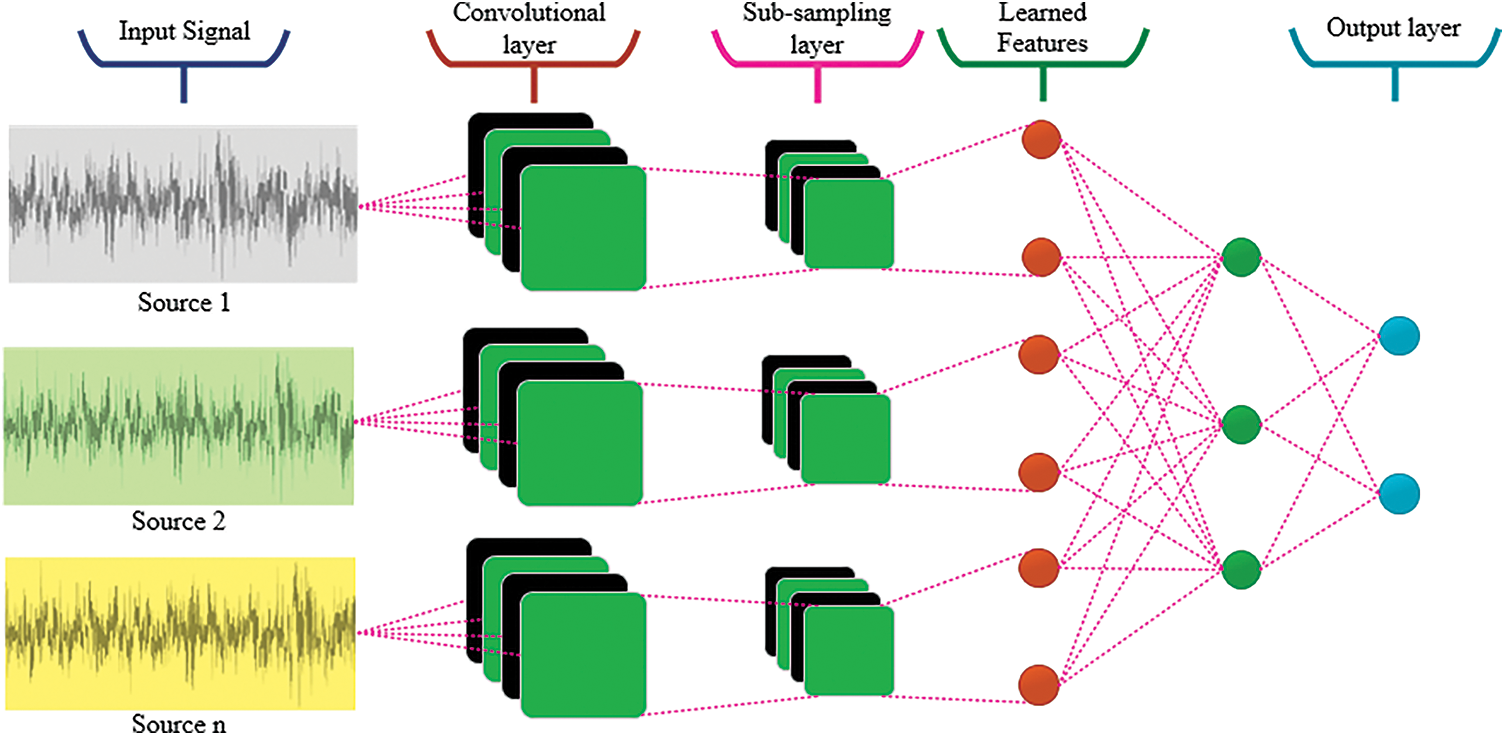
Figure 3: The execution process of CNN based architecture

4.4 Mayfly Optimization

The novel optimization technique introduced by Tsafarakis and Zervoudakis for providing enhanced results is Mayfly Algorithm (MA). The following steps illustrate the execution process of the MA optimization.

Step 1: Initialization

The first step of the Mayfly optimization is initialization where the populations of both male and female are initially x=[x1,…,xd] and y=[y1,…,yd] , respectively. These populations are considered as candidate solution that incorporated with d -dimensional vector. The proposed methodology is incorporated to select optimal learning by utilizing the mayfly optimization technique which helps to enhance the DCNN.

The mathematical formulation of objective function is shown below.

FF = Optimal Learning Rate (1)

The respective velocity is

v=[v1,…,vd] (2)

Step 2: Movement of Male

f(x) represents the global best position for the current iteration and it is marked as f(gbest). f(gbest) is denoted as global best position this is utilized for updating the next iteration and the Cartesian distance is calculated between the personal element and the global best agent gbest. The following equation provides the description.

xit+1=xit+vit+1 (3)

vijt+1=vijt+a1e−βrg2(gbestj−xijt)+a2e−βrp2(pbestij−xijt) (4)

where,

xijt => Agent i in dimension j at the current iteration t ,

vijt => Velocity,

a1 => Global learning coefficient,

a2 => Personal learning coefficient,

rg => Cartesian distance for global,

rp => Cartesian distance for personal,

Equation for the best agent’s velocity in the current iteration is derived below:

vt+1=vt+d×r

where,

d = > Nuptial dance,

r = > Random variable located in [−1, 1].

Step 3: Movement of Female

By analyzing the movement of the male’s mayfly, the female start to fly for breeding towards males. By considering the Cartesian distance between female and male, the velocities are updated.

vijt+1={vijt+a3e−βrmf2(xijt−yijt),iff(yi)>f(xi)vijt+fl×r,iff(yi)≤f(xi) (5)

where,

y = > Female agent,

a3 = > learning coefficient,

β = > Distance sight coefficient,

rmf = > Cartesian distance among with the female and male agent.

Moreover, based on the analysis of best male, the best females are arranged to match. Then next level females are arranged to match second-best male. Therefore, the male’s positions are significant in MA.

Step 4: Mating

In MA, offspring are generated from each couple where one part of them is configured to male population, whereas others are configured to female population.

Step 5: Updating

In updating phase, the weak solution is removed by best solution; this process is repeated until the expected outcome is reached.

The overall execution processes based on mayfly algorithm are clearly stated in the above algorithm. Based on aforementioned process and the results obtained in terms of performance analysis parameters, the proposed model seems to produce better outcomes.

5  Results and Discussion

By implementing the combination of DCNN with Mayfly optimization, the proposed model produces better results. This section mainly focuses on providing the results obtained based on the implementation of the work in MATLAB platform. The following section provides results in terms of accuracy, loss, SNR, MSE and NRMSE etc. This shows that the proposed model is effective in obtaining the expected outcome.

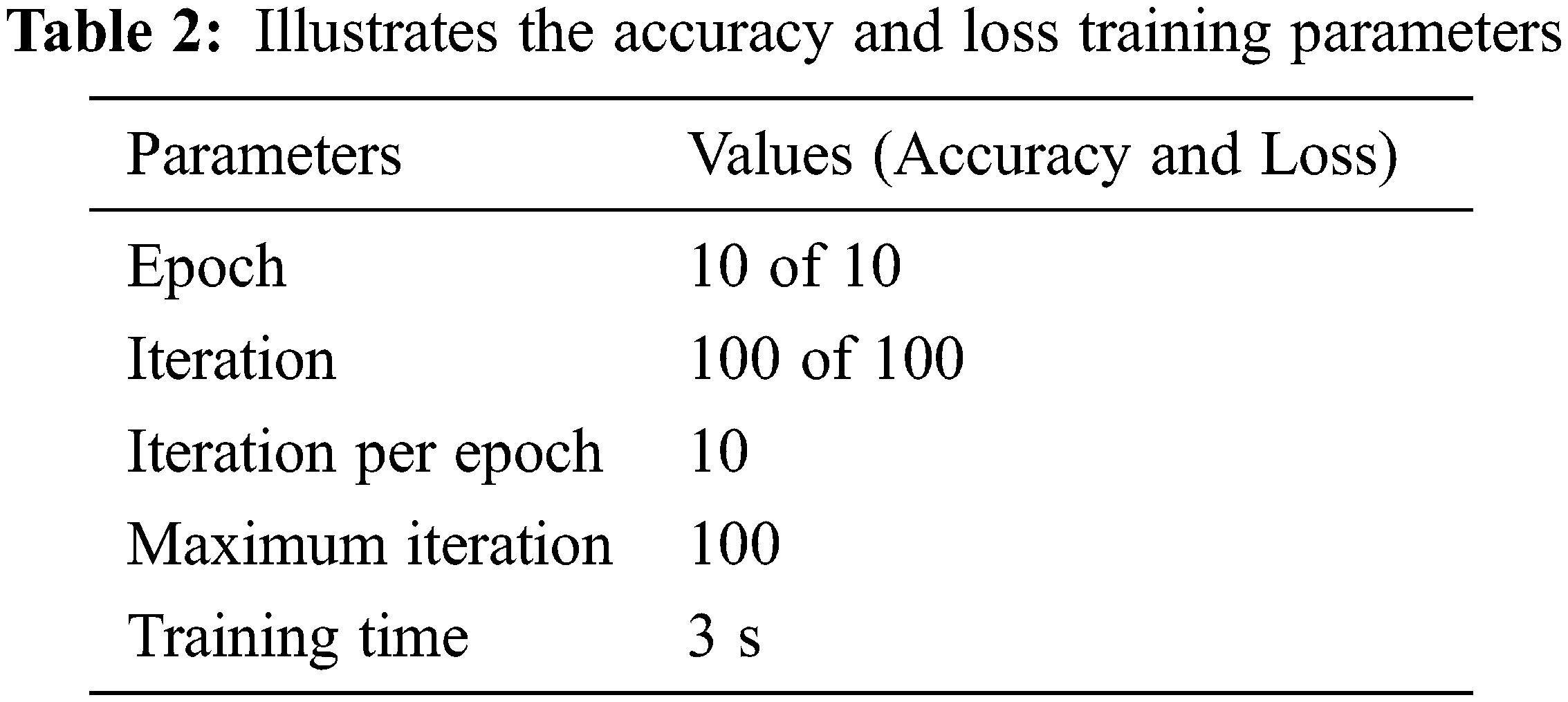
The results obtained in terms of loss are also shown which depicts that the proposed model incurred minimum loss. The Tab. 2 shows the type and training process in terms of accuracy and loss.

The Fig. 4 shows the results in terms of input data provided with the mean of 193.2847 and StD is 115.0069.

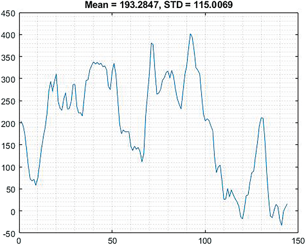
Figure 4: Shows the graphical representation of input data

The Fig. 5 shows the graphical image based on rank correlation with normalized data 0.9727.

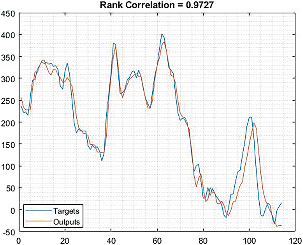
Figure 5: Shows the graphical representation of normalized data

In Fig. 5, the thick blue line represents smoothed and thin line represents unsmoothed during the training process. Similarly, in Fig. 6, the thick orange line represents smoothed and thin orange line represents unsmoothed.

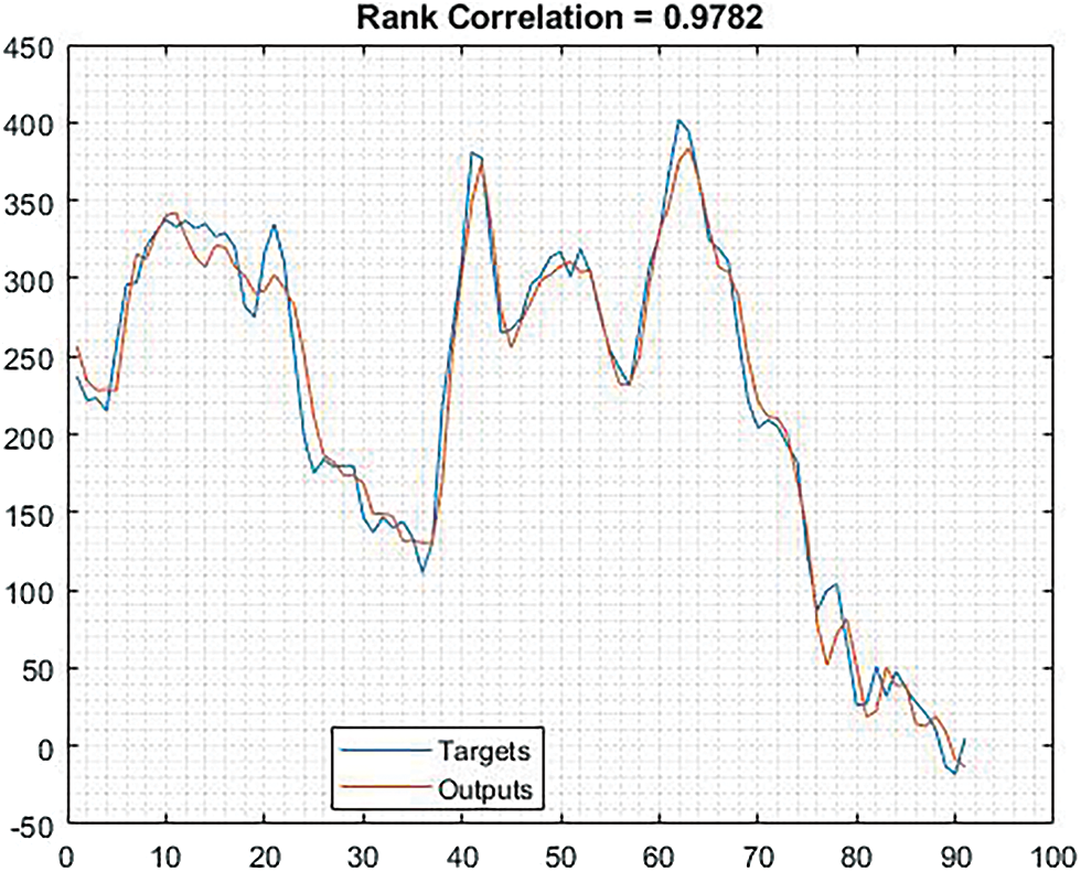
Figure 6: Shows the correlation based on rank correlation ratio

The Fig. 6 illustrates the rank correlation ration based on training values and prediction values. The result obtained based on rank correlation is 0.9782.

The Fig. 7 provides information about the error evaluation based on input signals which obtains MSE = 2820.637, RMSE = 53.1097, NRMSE = 0.84011.

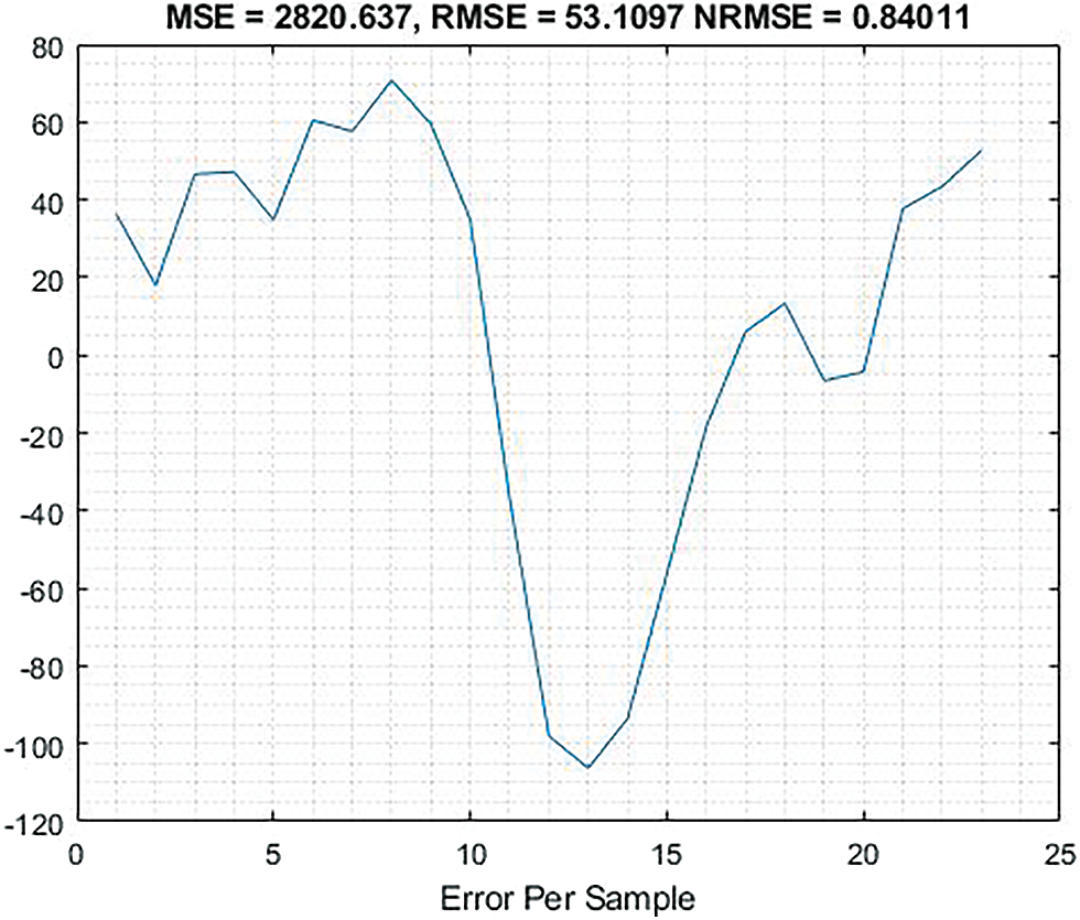
Figure 7: Shows the graphical representation of error evaluation based on input

The Fig. 8 provides information about the error evaluation based on output signals which shows MSE = 823.9263, RMSE = 28.7041, NRMSE = 0.14949.

Figure 8: Shows the graphical representation of error evaluation based on output

The Fig. 9 shows the Error Histogram Test which provides Error mean of 3.1232 and Error StD is 28.6597.

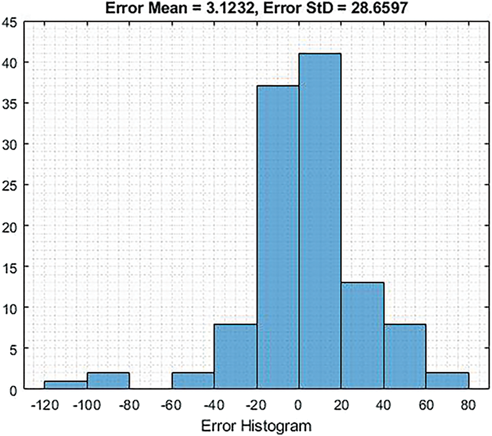
Figure 9: Shows the graphical representation of error histogram test

The Fig. 10 provides the graphical image of Error Histogram that provides error mean of 8.681, and error StD is 53.573.

Figure 10: Shows the graphical representation of error mean

The Fig. 11 shows that the graphical representation of function evaluation. The green graphical line indicates the estimated min objective and the blue line indicate that the min observed objective.

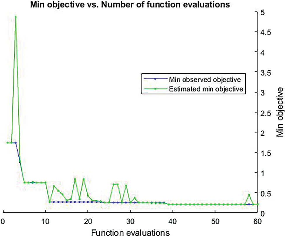
Figure 11: Shows the graphical representation of function evaluation

The Fig. 12 shows that histogram based on trained data. The results obtained in terms of error mean is 1.7184 and error StD is 17.8836.

Figure 12: Shows the graphical representation of histogram trained data

The Fig. 13 shows that the rank correlation based on trained data. The result obtained for rank correlation is 0.70232.

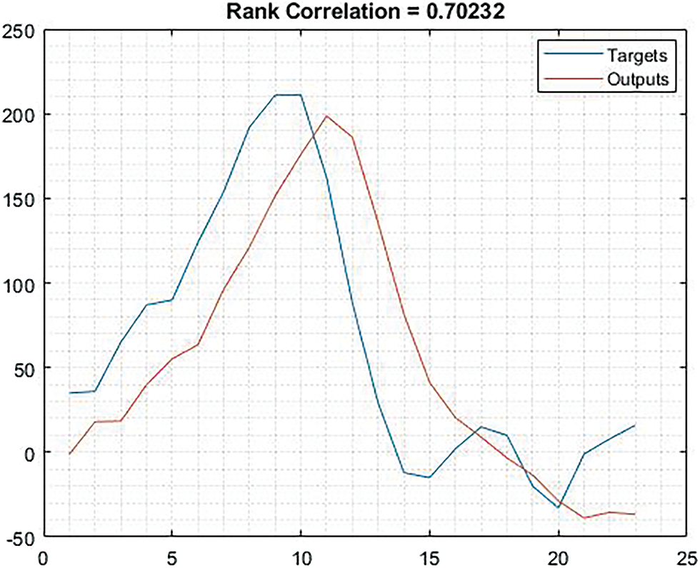
Figure 13: Shows the graphical representation of rank correlation

The Fig. 14 shows graphical representation of regression output which shows that the proposed model provides better results. The small circle in diagram illustrates the number of data, the linear line indicates fit, and the dot line is relying just near the fit line.

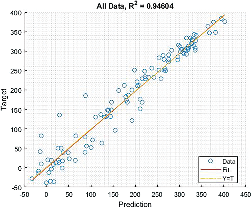
Figure 14: Shows the graphical representation of regression output

The Fig. 15 shows the graphical representation of SNR with a result of 23.67 dB in which the blue line represents the fundamental, the orange line represents the noise, and the black line represents the DC and Harmonics.

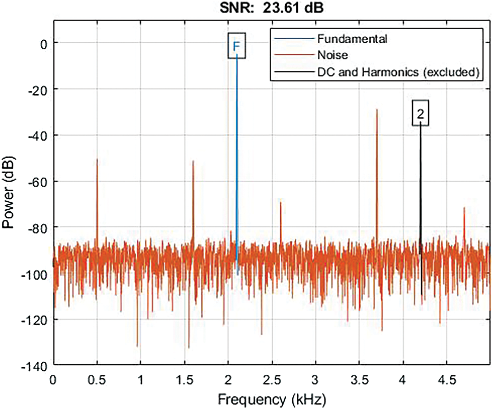
Figure 15: Shows the graphical representation of SNR

The below Figs. 16 and 17 illustrates the graphical results of proposed technique based on accuracy and loss respectively. It shows the proposed model has obtained 95% of accuracy.

Figure 16: Shows the graphical results of accuracy during training

Figure 17: Shows the graphical results of loss during training

6  Comparative Analysis

This section shows a comparative table obtained from different classifiers to prove the proposed model is better than other existing techniques. For this analysis, the classifiers based on detection of schizophrenia including SVM, SVM-RBF, LS-SVM, Decision Tree, KNN, DCNN, Proposed (CNN-MA) were used. The following Tab. 3 provides the comparative results based on proposed model.

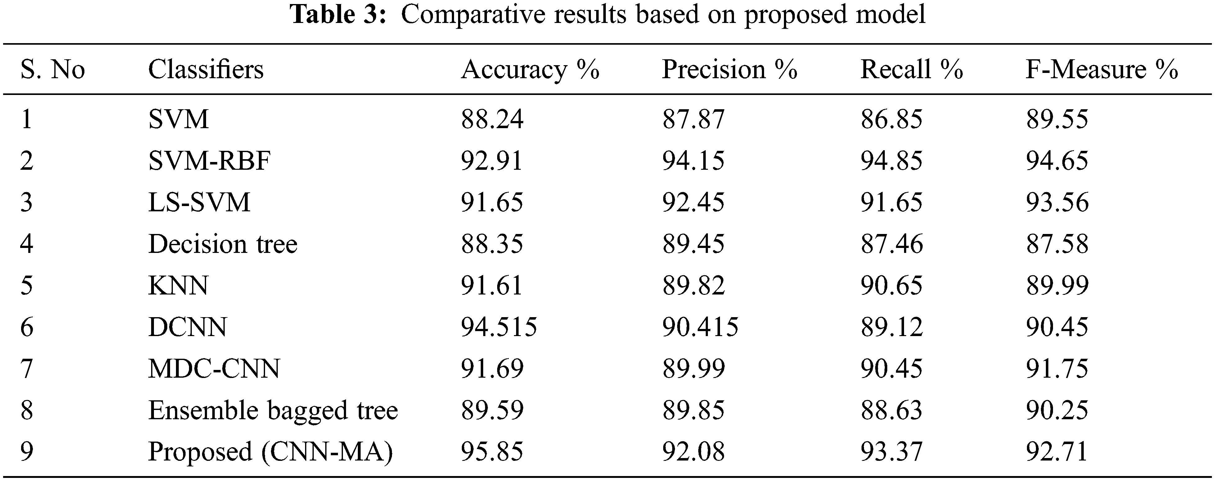
As per the above mentioned comparative results table, the performance of the proposed model is highly effective in terms of performance evaluation metrics such as accuracy, precision, recall, and f-measure. The comparative performance results shows that proposed model is better than the existing techniques.

7  Conclusion

This proposed technique is based on signal conducting system with EEG signals for diagnosing the schizophrenia disease. The ultimate purpose of the proposed model is to develop a novel technique to provide automated prediction system that helps in classifying the affected and non-affected people by utilizing the hybrid DL technique. This technique is incorporated with an excellent optimization technique namely Mayfly optimization which incorporates the functionalities of PSO and genetic algorithm. Therefore, the proposed model produces effective results. The implementation of this model is carried out in MATLAB platform and the results are obtained. Moreover, the obtained results including accuracy, loss, MSE, RMSE, MRMSE, etc. show that the proposed model is very effective in providing better outcomes. By this analysis, the proposed model is proved to be a better technique in predicting schizophrenia disease.

Funding Statement: The authors received no specific funding for this study.

Conflicts of Interest: The authors declare that they have no conflicts of interest to report regarding the present study.

References

1. B. Reza, K. Sadatnezhad and M. Sabeti, “An efficient classifier to diagnose of schizophrenia based on the EEG signals,” Expert Systems with Applications, vol. 36, no. 3, pp. 6492–6499, 2009. [Google Scholar]
2. S. Siuly, S. K. Khare, V. Bajaj, H. Wang and Y. Zhang, “A computerized method for automatic detection of schizophrenia using EEG signals,” IEEE Transactions on Neural Systems and Rehabilitation Engineering, vol. 28, no. 11, pp. 2390–2400, 2020. [Google Scholar]
3. A. Goshvarpour and A. Goshvarpour, “Schizophrenia diagnosis using innovative EEG feature-level fusion schemes,” Physical and Engineering Sciences in Medicine, vol. 43, no. 1, pp. 227–238, 2020. [Google Scholar]
4. M. S. Cetin, J. M. Houck, B. Rashid, O. Agacoglu and J. M. Stephen, “Multimodal classification of schizophrenia patients with MEG and fMRI data using static and dynamic connectivity measures,” Frontiers in Neuroscience, vol. 10, pp. 1–16, Oct. 2016. [Google Scholar]
5. L. Chu, R. Qiu, H. Liu, Z. Ling, T. Zhang et al., “Individual recognition in schizophrenia using deep learning methods with random forest and voting classifiers: Insights from resting state EEG streams,” arXiv preprint, 2017, arXiv:1707.03467. [Google Scholar]
6. A. Zhdanov, T. Hendler, L. Ungerleider and N. Intrator, “Machine Learning Framework for Inferring Cognitive State from Magnetoencephalographic (MEG) Signals,” in Advances in Cognitive Neurodynamics ICCN 2007, pp. 393–397. Springer, Dordrecht, 2008. [Google Scholar]
7. S. K. Prabhakar, H. Rajaguru and S. W. Lee, “A framework for schizophrenia EEG signal classification with nature inspired optimization algorithms,” IEEE Access 8, pp. 39875–39897, 2018. [Google Scholar]
8. M. Baradits, I. Bitter and P. Czobor, “Multivariate patterns of EEG microstate parameters and their role in the discrimination of patients with schizophrenia from healthy controls,” Psychiatry Research, vol. 288, pp. 112938, 2020. [Google Scholar]
9. U. Rajendra Acharya, S. L. Oh, Y. Hagiwara and J. H. Tan, “Automated EEG-based screening of depression using deep convolutional neural network,” Computer Methods and Programs in Biomedicine, vol. 161, pp. 103–113, 2018. [Google Scholar]
10. B. Thilakvathi, K. Bhanu and M. Malaippan, “EEG signal complexity analysis for schizophrenia during rest and mental activity,” Biomedical Research, vol. 28, pp. 1–9, 2017. [Google Scholar]
11. C. Devia, R. Mayol-Troncoso, J. Parrini, G. Orellana, A. Ruiz et al., “EEG classification during scene free-viewing for schizophrenia detection,” IEEE Transactions on Neural Systems and Rehabilitation Engineering, vol. 27, no. 6, pp. 1193–1199, 2019. [Google Scholar]
12. S. Miseon, H. J. Hwang, D. W. Kim, S. H. Lee and C. H. Im, “Machine-learning-based diagnosis of schizophrenia using combined sensor-level and source-level EEG features,” Schizophrenia Research, vol. 176, no. 2–3, pp. 314–319, 2016. [Google Scholar]
13. K. Oh, W. Kim, G. Shen, Y. Piao, N. I. Kang et al., “Classification of schizophrenia and normal controls using 3D convolutional neural network and outcome visualization,” Schizophrenia Research, vol. 212, pp. 186–195, 2019. [Google Scholar]
14. S. L. Oh, J. Vicnesh, E. J. Ciaccio, R. Yuvaraj and U. Rajendra Acharya, “Deep convolutional neural network model for automated diagnosis of schizophrenia using EEG signals,” Applied Sciences, vol. 9, no. 14, pp. 2870, 2019. [Google Scholar]
15. A. Sharma, J. K. Rai and R. P. Tewari, “Schizophrenia detection using biomarkers from electroencephalogram signals,” IETE Journal of Research, pp. 1–9, 2020. http://dx.doi.org/10.1080/03772063.2020.1753587. [Google Scholar]
16. C. R. Phang, C. M. Ting, F. Noman and H. Ombao, “Classification of EEG-based brain connectivity networks in schizophrenia using a multi-domain connectome convolutional neural network,” arXiv preprint, 2019, arXiv:1903.08858. [Google Scholar]
17. C. R. Phang, F. Noman, H. Hussain, C. M. Ting and H. Ombao, “A Multi-domain connectome convolutional neural network for identifying schizophrenia from EEG connectivity patterns,” IEEE Journal of Biomedical and Health Informatics, vol. 24, no. 5, pp. 1333–1343, 2019. [Google Scholar]
18. S. Mayo, L. M. Lorenzo, S. J. Revuelta and J. I. Arribas, “A Computer-aided diagnosis system with EEG based on the P3b wave during an auditory odd-ball task in schizophrenia,” IEEE Transactions on Biomedical Engineering, vol. 64, no. 2, pp. 395–407, 2016. [Google Scholar]
19. G. Li, D. Han, C. Wang, W. Hu, V. D. Calhoun et al., “Application of deep canonically correlated sparse autoencoder for the classification of schizophrenia,” Computer Methods and Programs in Biomedicine, vol. 183, pp. 105073, 2020. [Google Scholar]
20. T. Bose, S. D. Sivakumar and B. Kesavamurthy, “Identification of schizophrenia using EEG alpha band power during hyperventilation and post-hyperventilation,” Journal of Medical and Biological Engineering, vol. 36, no. 6, pp. 901–911, 2016. [Google Scholar]
21. M. Sabeti, R. Boostani, S. D. Katebi and G. W. Price, “Selection of relevant features for EEG signal classification of schizophrenic patients,” Biomedical Signal Processing and Control, vol. 2, no. 2, pp. 122–134, 2007. [Google Scholar]
22. S. K. Prabhakar, H. Rajaguru and S. H. Kim, “Schizophrenia EEG signal classification based on swarm intelligence computing,” Computational Intelligence and Neuroscience, vol. 2020, Article ID 8853835, 14 pages, 2020. [Google Scholar]
23. D. E. Rumelhart, G. E. Hinton and R. J. Williams, “Learning representations by back-propagating errors,” Nature, vol. 323, no. 6088, pp. 533–536, 1986. [Google Scholar]
24. Y. LeCun, Y. Bengio and G. Hinton, “Deep learning,” Nature, vol. 521, no. 436, pp. 436–444, 2015. [Google Scholar]
25. J. Fu, S. Yang and F. He, “Sch-net: A deep learning architecture for automatic detection of schizophrenia,” BioMedical Engineering OnLine, vol. 20, no. 75, pp. 1–21, 2021. [Google Scholar]
26. J. W. Kim, Y. S. Lee, D. H. Han, K. J. Min, J. Lee et al., “Diagnostic utility of quantitative EEG in un-medicated schizophrenia,” Neuroscience Letters, vol. 589, pp. 126–131, 2015. [Google Scholar]
27. A. Zülfikar and A. Mehmet, “A deep learning approach in automated detection of schizophrenia using scalogram images of EEG signals,” Physical and Engineering Sciences in Medicine, vol. 20, no. 5, pp. 83–96, 2021, https://doi.org/10.1007/s13246-021-01083-2. [Google Scholar]
28. Z. D. Aharon, N. Fogelson, A. Peled and N. Intrator, “Schizophrenia detection and classification by advanced analysis of EEG recordings using a single electrode approach,” PLoS One, vol. 10, no. 4, pp. 1–12, 2015, https://doi.org/10.1371/journal.pone.0123033. [Google Scholar]
29. A. Zulfikar and A. Mehmet, “Automatic detection of schizophrenia by applying deep learning over spectrogram images of EEG signals,” Traitement du Signal, vol. 37, no. 2, pp. 235–244, 2020. [Google Scholar]
30. C. A. Torres Naira and C. J. L. Del Alamo, “Classification of people who suffer schizophrenia and healthy people by EEG signals using deep learning,” International Journal of Advanced Computer Science and Applications, vol. 10, no. 10, pp. 511–516, 2019. [Google Scholar]
Cite This Article
Copyright © 2023 The Author(s). Published by Tech Science Press.
This work is licensed under a Creative Commons Attribution 4.0 International License , which permits unrestricted use, distribution, and reproduction in any medium, provided the original work is properly cited.
Downloads
Citation Tools