Optimizing Storage for Energy Conservation in Tracking Wireless Sensor Network Objects

1  Introduction

The advancement of electrical and wireless communication technologies has resulted in the creation of wireless sensor nodes in recent years. Sensors, processor, memory, connection, and power components are all included in a conventional sensor node. Most of the time, they are equipped with a battery. However, in several circumstances, repairing a battery is not only expensive but often impracticable. Simultaneously, many WSN applications demand that the network to provide Quality of Service (QoS), such as minimal query latencies and a strong likelihood of a valid query. As a result, energy economy and QoS are important concerns in the development of complex WSNs. Object tracking is a prevalent activity in WSN applications. The position of the identified object is required in such applications.

When a node senses an activity, it has the option of recording it in its local memory or broadcasting that to its neighboring nodes. Since the targeted object may travel inside the surveillance region, a single sensor will not be able to track the underlying object autonomously. Four additional sensors are needed to reveal the exact position whenever a sensor senses an object inside its detecting region. In conventional object tracking studies, the difficulties about how to choose acceptable sensors to identify and aggregate information, as well as how to inform appropriate sensors to stay up for subsequent observation, are major concerns. The majority of object tracking applications need a real-time geolocation update. Other applications, on the other hand, require the whole or partial history motion data of the identified object. For instance, army requires the attacker’s trajectories information to assess the enemy’s activities on the battleground. Whenever a warrior subsequently reaches the tracked battleground, he will be able to see the attacker’s historic position. WSNs segregate object tracking strategies into cluster-based and non-cluster-based approaches. Whenever a non-cluster head sensor senses an object in cluster-based protocols [1], it transmits messages to its cluster head. The cluster head gathers data and pass it to a sink. This method decreases the needed connection capacity as well as the amount of energy used. In WSNs, there is no node that serves as cluster head in non-cluster-based protocols. Whenever an object is sensed, it stores its movement data in its local memory. Whenever a consumer needs to know the position of a monitored object, he or she makes a query to WSNs. To retain information of earlier attackers, the WSN requires specific storage strategies. External, internal, and data-oriented storage are the three types of data storage systems discussed in the study [2]. Every sensor transmits all obtained information to a sink in the external memory. This data retention strategy could run into some issues. Whenever the sink node that initially had the gathered data retires or shuts down, all its data must be transferred to a fresh sink node so that consumers may use it thereafter. External memory strategy underperforms for applications that demand a mobile sink. There are two major drawbacks to using external memory. Firstly, the capacity of memory required at the sink node is massive. Secondly, every node must send its data to the sink node, which might use a significant bandwidth capacity. Whenever the system senses an activity, it holds the data in its internal memory. As users must access the whole sensor network, this storage strategy is inefficient. In data-oriented storage, the underlying data is retained in accordance with its respective data type. A data node is designated to hold the data belonging to same type. Further, users will post data retrieval queries to these data nodes based on the type of data. On the contrary, many control messages are necessary since the object is roaming.

1.1 Motivation

Object tracking in WSN needs continuous monitoring of an object’s location [3–15]. The object should be found initially, and its course must be followed as it travels all around sensing area. In this work, we target on the data management challenge in order to assist users in successfully querying object tracking and obtaining the object position, and thus conserving energy. Object tracking in WSN require specific storage strategies to save data about moving objects. There are several data structures [16–21] available for data management; however, the current research is focused on developing a more efficient (with logarithmic complexity) data structure (based on linked list) to preserve more energy in WSNs.

1.2 Research Contribution

In this research, we target the data storage challenge to assist users in efficiently querying object tracking and obtaining the object position, and thus conserving energy. We designed a novel linked-list based data storage and its access mechanism that is more efficient than the linked list structure adopted in [15]. In this work, the suggested data structure, the Ordered Binary Linked List (OBLL), can execute dynamic set operations in logarithmic time while preserving its operations and structural simplicity. The suggested OBLL structure possesses both the Min Heap and Max Heap properties [22]. The OBLL, like the Min Heap’s Find-Minimum and Max Heap’s Find-Maximum operations, performs both of these operations in O(1) time. Because the complexity of putting an element in an n-element heap is log2n, the identical operation in an n-element OBLL has a lower complexity. In addition, the Extract-Minimum and Extract-Maximum procedures may be completed in less time.

2  Literature Review

Considering various lightweight gadgets including cellphones, notebook, and laptops are frequently employed to access the Web all across the globe [23], WSN plays a critical role in this revolution. Majid et al. [24] conducted a comprehensive literature evaluation that covers a wide variety of topics related to Industry 4.0, identifies investigation inadequacies, and makes recommendations for future study. It includes a variety of topics related to Industry 4.0, including the design process, security requirements, network deployment, system categorization, obstacles, constraints, and possible trends. As the rate of modernization rises, the need to automate different individuals has become increasingly important for growth. The information generated by Smart must be handled properly and securely. The methodology developed by Somayaji et al. [25] might assist policymakers in planning ahead of time to put purchases for removable battery, ensuring seamless services. Dev et al. [26] attempted to enhance power consumption in networks by choosing the best cluster head utilizing new evolving nature-inspired methodology. The suggested model increases the lifespan of the network by maintaining many nodes active. Further, Roy et al. [27] suggested a technique the enables privacy preservation with minimal verification latency during handover activity, based on experimental findings. Chéour et al. [28] propose a power usage optimizer titled “Hybrid Energy-Efficient Power Manager Scheduling” (HEEPS) tailored to the needs of WSNs. The suggested power regulator is unique in that it combines many approaches, including time-out Dynamic Power Management, Dynamic Voltage and Frequency Scaling, and the Global Earliest Deadline First (GEDF) scheduler, to achieve greater scheduling efficiency. Pang et al. [29] investigated to save energy in WSNs for object tracking. This study included three types of precautionary measures to reduce energy consumption: Ensuring optimal management system, prolonging the elapsed time between two neighboring occurrences, which could save detecting and interacting energy, and preferentially conveying findings, potentially saving interacting energy. The goal of this study is to address the data storage challenge by assisting users in rapidly querying object tracking and retrieving object position while conserving energy. As a result, we divided our literature review into two sections i.e., 1) Object Tracking in WSN and 2) Data Structure

2.1 Object Tracking in WSN

Tseng et al. presented a new mobile agent-based approach [3]. When a new item is identified, a mobile agent is launched to follow the object’s wandering route. The mobile agent shall select and remain in the sensor proximal to the monitored object. To complete the duty of object tracking, the mobile agent collaborates with its neighbors and spreads the item’s position to the sink node. To conserve energy, the amount of the data traffic [4], connection requests [5], participating sensors or data transmitted to cluster head, needs to be limited [6]. Alternatively balancing the use of energy can be achieved through mobile sinks [7]. Prediction-based approaches [8,9] are adopted to anticipate the position of movable objects for conserving energy. Whenever a sensor senses an object, it transmits the related data including object’s position, speed, and travelling orientation to the cluster head. The cluster head evaluates and forecasts the object’s position before broadcasting wakeup data to the expected region. This technique conserves energy as it reduces the number of active nodes. Unfortunately, whenever the multicast technique encounters an empty grid in the WSN and position refresh traffic is not lowered, object tracking can collapse. Prediction-based monitoring for object tracking has been suggested in [10], that employs forecasting to decrease position refresh frequency. However, the effectiveness of the forecasting model is dependent on its precision. In practical uses, getting an effective forecasting model is challenging since the object can wander at arbitrary. Simultaneously, upgrading the forecasting models necessitates a significant amount of additional traffic. Object tracking in WSN, as previously mentioned, require specific storage strategies to save data about moving objects. A tree-based distributed position database is presented in [11], wherein every database unit spans a specified area and contains geolocation data for all objects existing within it covered area. A position tree pattern is developed by the distributed position database. To decrease the message transmission expense related to position updates, a deviation avoidance and highest weight first approach is presented in [12] to build an object tracking tree. However, establishing a position tree incurs additional energy costs, and tracking data is not shared with consumers.

Energy-conserving Approximate storage (EASE) is presented in [13] to save two variants of objects’ position information. To decrease protracted traffic caused by distant updates, highly precise data is maintained at an internal storage node that is near to a traveling object. Simultaneously, to decrease query latency, the same information with a low precision is duplicated to select appropriate storage nodes that are accessible to consumers. As a result, if a query’s precision requirement is lower than the approximate precision, the query is handled by the assigned storage node. If the query cannot be resolved locally, it is sent to the internal storage node. By decreasing both update and query traffic, EASE improves network efficiency. However, since the query data should be sent to the appropriate storage node and subsequently to the internal storage node, the query delay for highly precise queries is significant. Further, it is incapable of properly monitoring queries. Data gathering and computation latencies are acceptable by certain object tracking software. A delay-tolerant trajectory compression (DTTC) was suggested [14] to exploit the delay acceptance. Inside the DTTC system, a cluster-based architecture is created. Every cluster head uses a compression mechanism to condense an object’s travel path inside its cluster. The cluster head solely sends the compaction attributes to the sink node, that offers expressive yet identifiable representations of the object’s motions to the sink node. They further considerably decrease the amount of data transfer necessary for tracking activities.

Ho et al. presented an energy efficient technique entitled Energy Efficient Data Storage (EEDS) that may be used in WSN software demanding to retain past data of mobile objects [15]. The primary concept is to construct a linked list along with an object’s traveling route and query on it to capture all information corresponding to an object with minimal control cost. This technique makes advantage of internal storage and does not require any query requests to be flooded. Attributed to the reason that the linked list has only single entry point, all query operations should traverse the linked list from the starting node to receive a result. As a result, due to delay and a huge amount of energy loss, it can’t handle real time position queries and partial history path queries effectively, particularly whenever the linked list size is quite huge.

2.2 Data Structures

Aside from the many advancements in the computer sector, storing data while it is being processed has always been a major problem. By applying the usage of multiple data structures, computer scientists have developed an effective solution to the problem. Arrays are commonly used to store large amounts of data [16]. The benefits of utilizing an array are that we don’t have to create separate identifiers (IDs) for each item of data; instead, we just need one identity and its index to access all the data. Second, data is saved in a contiguous way in the primary storage device. Static memory allocation is the name for this form of memory allocation. Later, to get around the array’s restrictions, we employed different forms of lists, such as single, double, and circular lists. To avoid naming issues and to adhere to the idea of dynamic memory allocations [17], these lists do not have separate IDs for their nodes, and the nodes are accessible by their addresses. These arrays and lists can perform the most fundamental dynamic set operations including insertion, deletion, searching, and traversal in linear time. By combining these data storage methods with the application of the Last in First out (LIFO) and First in First Out (FIFO) concepts, stack and queue data structures may be created. Furthermore, the creation of tree data structures attempted to achieve logarithmic complexity for various operations, but the idea of binary search tree (BST) failed with a certain type of input and displayed linearity in its structure [18]. Our BST data structure was no better than the lists in this case. We must balance the BST [18] to preserve logarithmic complexity in most dynamic set operations. The answers to these difficulties are the Adelson-Velskii and Landis (AVL) tree [19] and Red-Black (RB) tree [20], which are also known as self-balancing trees. We created a new data structure called Heap [21] by altering the notion of trees. Heap may be divided into two types: Max heap and Min heap. The Min and Max heap concepts assisted us in sorting our input components efficiently and at a total time cost of O(nlog2n), which was favorably received and gained amazing popularity in the research community. Although the heap was faster at producing sorted sequences, it failed to construct both rising and decreasing sequences using a single data structure. It indicates that if we want to produce a non-decreasing series, we should use the Min heap structure, and if we want to build a non-increasing sequence, we should use the Max heap structure.

3  Materials and Methods

It is necessary to define the different terminology and structure of OBLL before proceeding with the detailed description. OBLL is made up of several doubly circular linked lists. The root list is the initial list in the OBLL. Nodes in the list can have children, which are referred to as child nodes, and the list linked to any node is referred to as the child list of that node. The pointer “start” points to the very first node in the root list. The order determines the structure of OBLL (represented by t). The order of the OBLL determines the number of nodes that can be held by each list and the maximum number of nodes that can be held by each list. OBLL has a somewhat different idea of data structure node allocation. We’ve been utilizing several data structures with preset formats up until now. As a result, it was necessary to adhere to it. OBLL is unusual in that it provides two distinct sorts of nodes at the same time. These nodes differ from one another in a few pointer and data fields. Both nodes are employed depending on the situation’s demand and need. Augmented Node (or heavy node) and Normal Node are the two types of nodes (or light node) as presented in Fig. 1. In this study, augmented nodes are depicted as shaded nodes to distinguish them from normal nodes. Because it has more fields than a standard node, augmented nodes are referred to as hefty nodes. The list’s initial node is the only one that has been enhanced. Parent (pointing to the parent of the node), Child (pointing to the child node), Key (the data field storing the information), Count (the data field storing the count of the number of nodes in the list), Previous written as prev (pointing to the previous node in the list), and Next (pointing to the next node in the list) are the fields in the augmented node (pointing to the next node in the list). The typical node is quite similar to the nodes that were previously utilized in data structures. Node has fields named next, prev, child (the pointer fields) and key (the data field). Their use and features are same as that of augmented node.

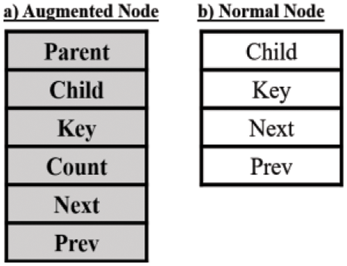
Figure 1: a) Structure of an augmented node and b) Structure of normal node

The following are some of the OBLL’s characteristics or constraints:

■   In the OBLL, every list is a doubly linked list

■   Any list can have a maximum number of nodes equal to the OBLL order (t).

■   The OBLL’s order (t) must be greater than 3 (i.e., t>=3).

■   Until the current list meets the criterion of having the maximum number of nodes, none of the nodes in it can own the child list or child node.

■   The nodes in the OBLL list are ordered in ascending order.

■   The nodes in the child lists are larger than their parent node but smaller than their parent node’s sibling (Next of their Parent).

■   Any list’s last node does not have a child node.

3.1 Dynamic Operations

The core dynamic operations that a data structure must provide are creation, insertion, searching, deletion, and traversing.

3.1.1 Creation Operation

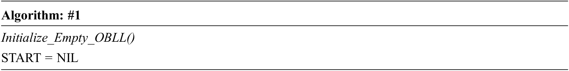
Creation operation in OBLL is defined under three dimensions viz. 1) creation of OBLL, 2) creation of an augmented node, and 3) creation of normal node. We represent the OBLL with an identifier named “start”. This identifier is initialized by “nil” in the beginning using Algorithm #1. Further to create an empty augmented node and normal node, Algorithm #2 and Algorithm #3 are adopted respectively.

3.1.2 Insertion Operation

While inserting a node in OBLL it is checked that property 2, 4, 5, 6, 7 (stated above) are not violated. We shall not advance further in a list’s child list if the number of nodes in the list does not match the order of the structure; instead, we will add the node in the same list at the proper place. This will prevent the overall structure from becoming linear when the branching is expanded. The insertion process (depicted in the Algorithm #4 i.e., Insert_OBLL) starts with locating the insertion point in the OBLL structure. If the COUNT of OBLL structured list (SL) i.e., the current list is less than t, insertion occurs in SL; otherwise, the insertion operation is called recursively on the child list of an applicable SL node.

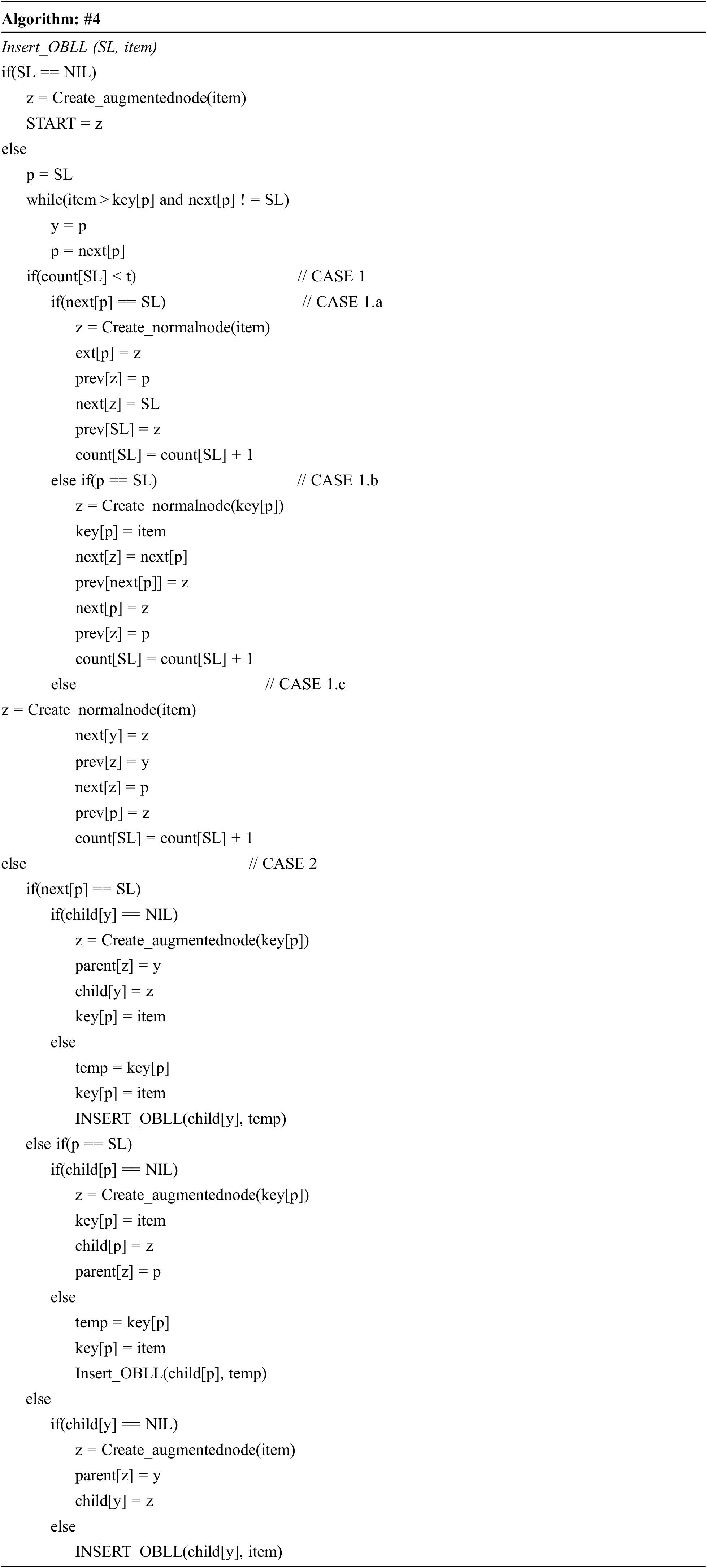
The entire insertion procedure may be divided into two primary scenarios to better comprehend it. Consider the SL pointer, which denotes the current working list and contains the address of the list’s first node. During the insertion procedure, two pointers labelled ‘p’ and ‘y’ are kept track of. For putting up a new node (with key = item) in SL, we must traverse the SL and locate a suitable node in which Key[y] < item < Key[p].

CASE 1: count[SL]<t

The main characteristic of case 1 is that it shows that the COUNT of SL is smaller than t, implying that the new node would be inserted into the same existing list SL. This case is divided into three sub-cases.

■   CASE 1.a: next[p] =SL

The node to be inserted has the greatest value of all the nodes in the list, and it is to be placed at the end of the list SL.

■   CASE 1.b: p=SL

When the searching comes to an end with p=SL, it means that insertion will take place at the beginning of the current list SL, with the item having the smallest value of all the nodes in SL.

■   CASE 1.c: anywhere in the middle of SL

The typical insertion, which takes place somewhere in the centre of the current working list SL, is the third case. Between p and y, a newly created node with data is sandwiched.

CASE 2: count[SL]=t

The second scenario occurs when SL is entirely filled and the number of nodes equals the structure’s order; in this case, control must be diverted downwards in the branch or any child lists of SL. It’s important to note that, despite the fact that the insertion process is divided into two primary instances, case 2 is primarily responsible for recursively migrating the control along the branch. In example 2, insertion simply determines the suitable location for y and p and calls the insertion process on the child of y recursively. It is either case 1 or case 2 of insertion method when it is asked to insert a node in a specified OBLL with n nodes. Case 2 is the one that recursively calls the process. The length of any list is at most t, and the depth of the OBLL is at most logtn, according to the structure of the OBLL. As a result, the worst-case complexity of inserting a new node is O (t logtn), which may be written as O (logtn) if t is assumed constant.

While inserting the 50, 5, 40, 10, 8, 12, 25, 19, 41, 110, 35, 37, 42, 17, 65, 58, 70, 74, 6, 2, 130 keys, several cases of insertion algorithm are illustrated in Fig. 2.

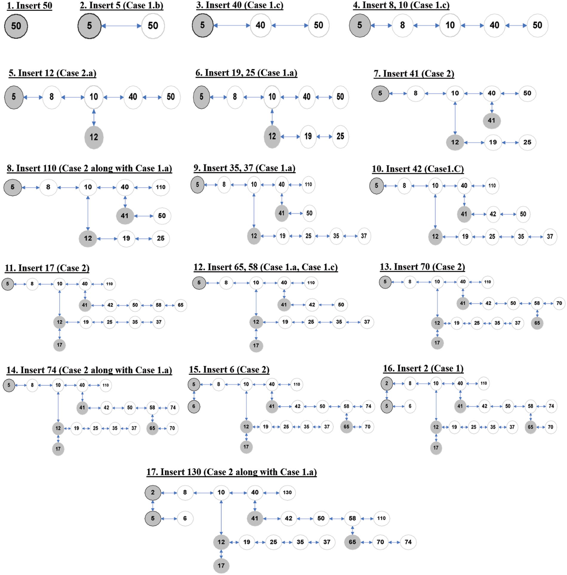
Figure 2: Various cases of insertion in OBLL for the sequence 50, 5, 40, 10, 8, 12, 25, 19, 41, 110, 35, 37, 42, 17, 65, 58, 70, 74, 6, 2, 130 (NOTE: For visual clarity, the circular linked list is not displayed in the graphics at the conclusion of the nodes.)

3.1.3 Searching Operation

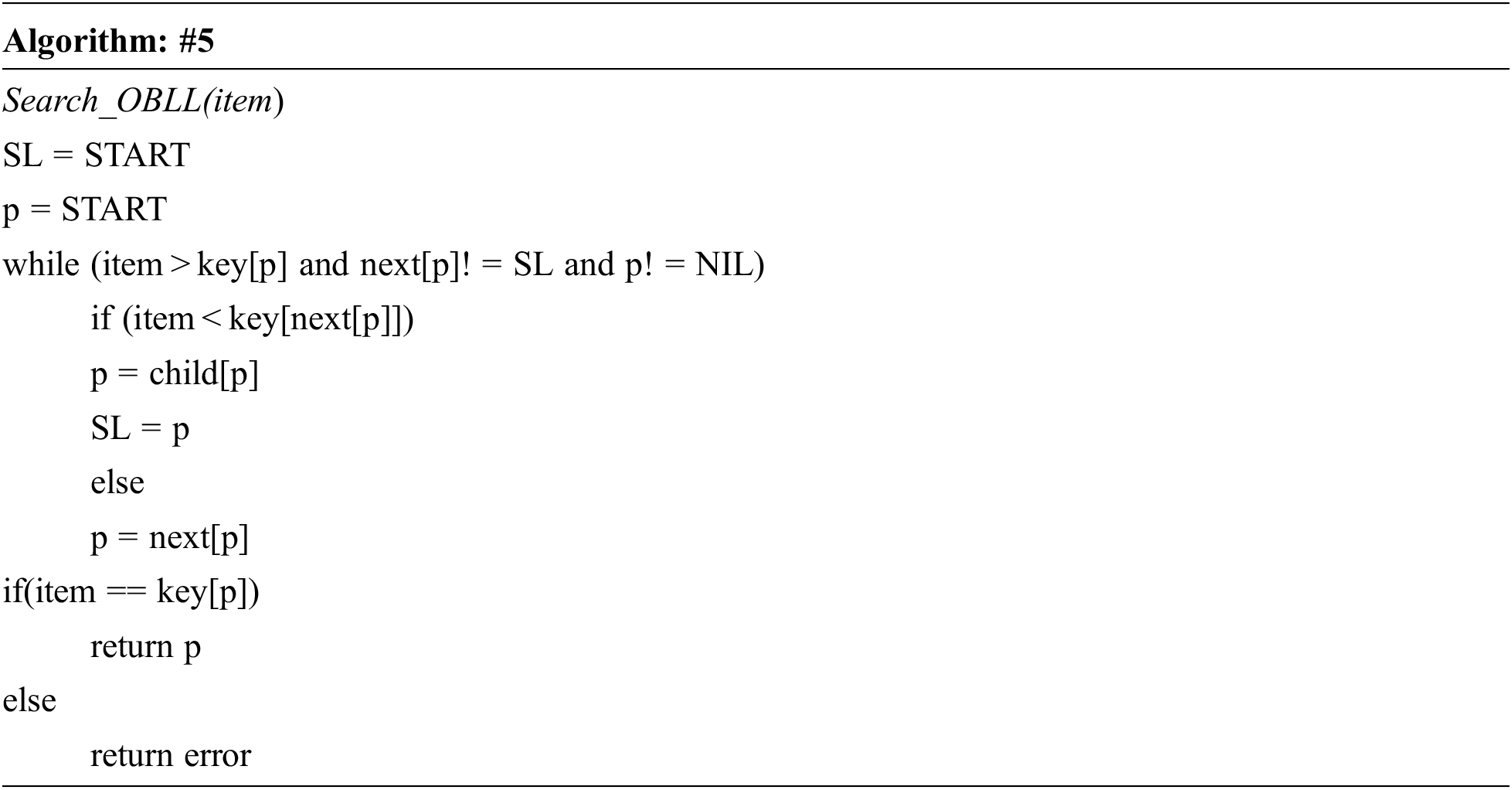
In addition to linear search in the current list, branching in OBLL may be used at any time to go down in the structure as presented in the Algorithm #8 i.e., Search_OBLL. The search begins with the “START” list, and SL refers to the current working list in the process. In the while loop, verify that the value to be searched is higher than the value of pointer ‘p’ (current node). If the value inside the while loop falls below the value of next[p], SL advances to the child list of p, otherwise the linear search continues. If the search is successful, SEARCH_OBLL provides the node’s address with key[node]=item; otherwise, it gives an error, i.e., next[p] becomes equal to SL (reaches the end of the list) or p becomes equal to NIL (reaches the end of the child list). The complexity of finding an element in the OBLL is O(logtn).

3.1.4 Deletion Operation

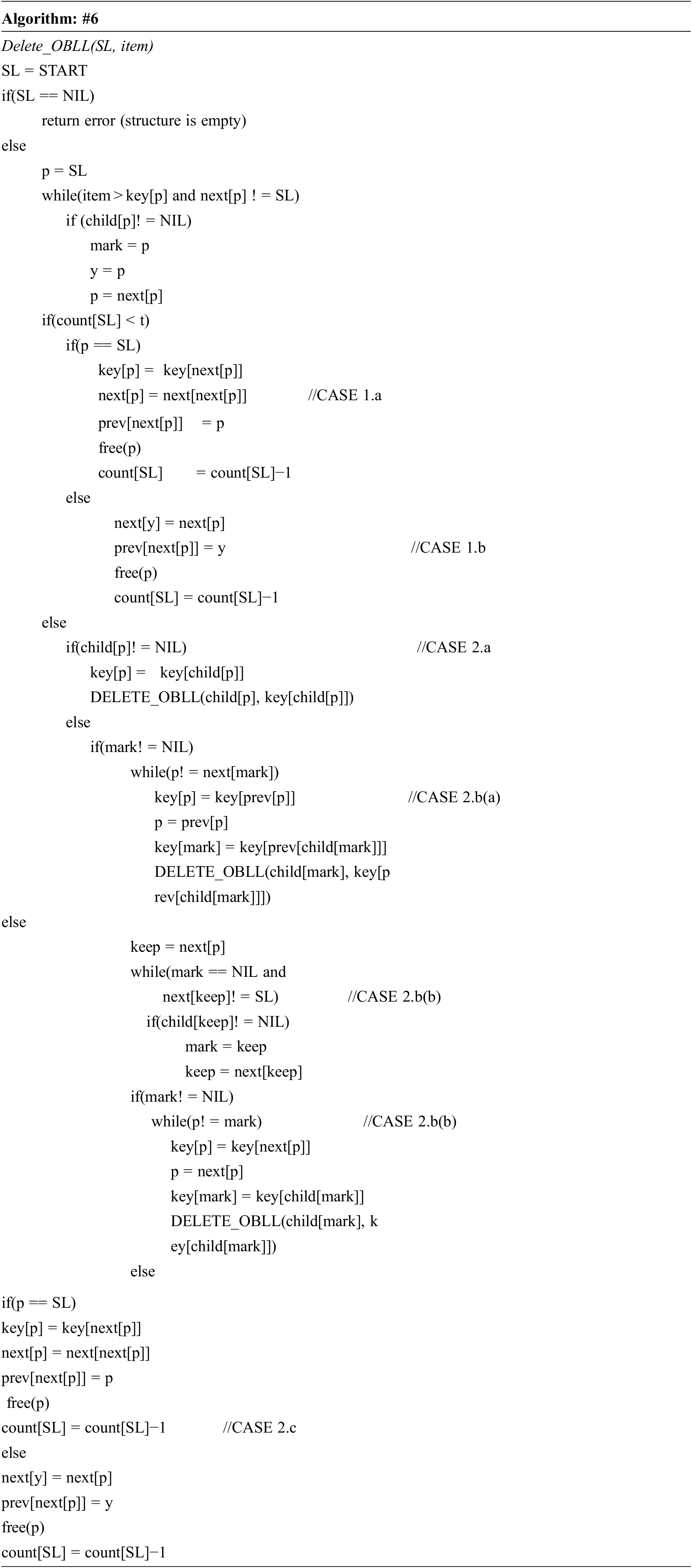
In OBLL, the deletion process is a little more complicated than the insertion process. The first and most important thing to remember when deleting a node is that it must not contradict properties 4 and 7. Property 4 prevents any node from being deleted from a completely filled list if any of the nodes in that list has a child node.

Property 7 prevents the last node in a completely filled list from being deleted if any of the other nodes in the list contains a child node. As a result, attributes 4 and 7 disallow physical deletion of either the list’s final node or the node containing the child node. As a result, attributes 4 and 7 disallow physical deletion of either the list’s final node or the node containing the child node. This assures that if a list contains any child lists, it will never be deleted. Rather, we may argue that removing a node physically removes a node from the node’s lowest list. The deletion of any node physically occurs from the bottom most of the OBLL structure, which is a straightforward approach to handle or face the above stated problem. The primary goal of deletion is not just to physically delete any node, but also to prevent the linearity that branching causes in the overall structure. A pointer SL denotes the current working list and contains the address of the list’s first node.

The deletion procedure is divided into two stages. The first step looks for the correct node to delete, and the second phase deletes the nodes from the data structure. We keep two pointers designated ‘p’ and ‘y’ during the search operation in the deletion procedure. The pointer referring to the current node is ‘p,’ while the pointer pointing to the previous node is ‘y.’ The phenomenon of complete deletion may be divided into two categories.

CASE 1: count[SL] < t

When count[SL]t is used, it means that a node must be removed from a list, such as SL, where the number of nodes in SL is fewer than the structure’s order. In this example, property 4 and 7 violations are unimportant because the list SL will not include any child lists. This case is split into two sub-cases.

■   CASE 1.a: p =SL

When the first node of SL is to be destroyed, instead of removing node p, the values of p are swapped with those of next[p], and next[p] is deleted. As a result, node p is conceptually removed from the structure, while node next[p] is actually removed.

■   CASE 1.b: p is any other node in SL

This scenario is straightforward: we just connect prev[p] and next[p], and node p is physically removed from the structure.

CASE 2: count[SL] =t

In this scenario, the deletion procedure gets complicated, and properties 4 and 7 are likely to be violated. This case is divided into three sub-cases to make it easier to comprehend.

■   CASE 2.a: Child[p]! = NIL

If the node to be removed has a child list, just copy the value of the child node of p into node p, then use Delete_OBLL (SL, item) recursively over the child node of p.

■   CASE 2.b: child[p]=NIL

If the pointer p to the to be deleted node does not have a child node, the node p cannot be destroyed immediately since the current list is complete and any other node might have a child node. To solve this problem, OBLL keeps another pointer termed mark, which points to the first node with a child that is closest to p when scanning to the left of p. If the left scan fails to locate such a node, a right scan is conducted to locate a node with a child.

o   Case 2.b(a): When mark is to the left of p

Starting with node p and proceeding to its left, the keys of the nodes are moved with the values of their previous nodes. At the next of mark, the process of changing the key values will come to an end. The child list of mark node is now examined, and the key of its last node (identified as the prev of the child node) is copied into mark node’s next. The recursive Delete_OBLL function is then run on the last node of the mark node’s child list.

o   Case 2.b (b): When mark is to the right of p

The keys from mark to p are moved to their left nodes in this example. At p, the shifting process will come to an end. Finally, the key of mark is swapped out for the key of mark’s child node. On the child of the mark node, the recursive operation DELETE _OBLL is invoked.

■   CASE 2.c: When mark is nil

It’s also possible that none of the nodes in the current list include the child list, in which case the situation is similar to CASE 1 and p is deleted as in CASE 1. The complexity of removing any element from OBLL is O (t logtn), where t is constant and may be disregarded, resulting in a complexity of O (logtn) for deletion.

An example to illustrate various scenarios of deletion operation is presented in Fig. 3. Step 1 of Fig. 3 presents an OBLL of order 5. Step 2 in Fig. 3 depicts the case of deleting key 65. In this scenario, p begins pointing to the node in Fig. 3 with key element 65. This node belongs to a list with less than t nodes. Aside from that, p is the first node in its own list, thus it’s deletion case 1(a). Step 3 in Fig. 3 depicts the case of deleting key 74. In this scenario, p begins pointing to the node with key element 74. This node belongs to a list with less than t nodes. Furthermore, because p is not the first node in its own list, case 1(b) of the deletion method applies. In step 4 of Fig. 3, the Algorithm #6 i.e., Delete_OBLL is invoked on the node with key element 10. It is case 2(a) of deletion since this node has a child node and is a member of a list that also contains t nodes. In this situation, the key of the child node, i.e., 12, is duplicated into the key element 10 of the node, and then Delete_OBLL is called recursively on the node on which the child node of p is located. Case 2(a) occurs once more on a child node with key element 12; the 17 is transferred to the node with key value 12 and Delete_OBLL is invoked recursively on the node with key element 17. It’s case 1(a) of the deletion method this time.

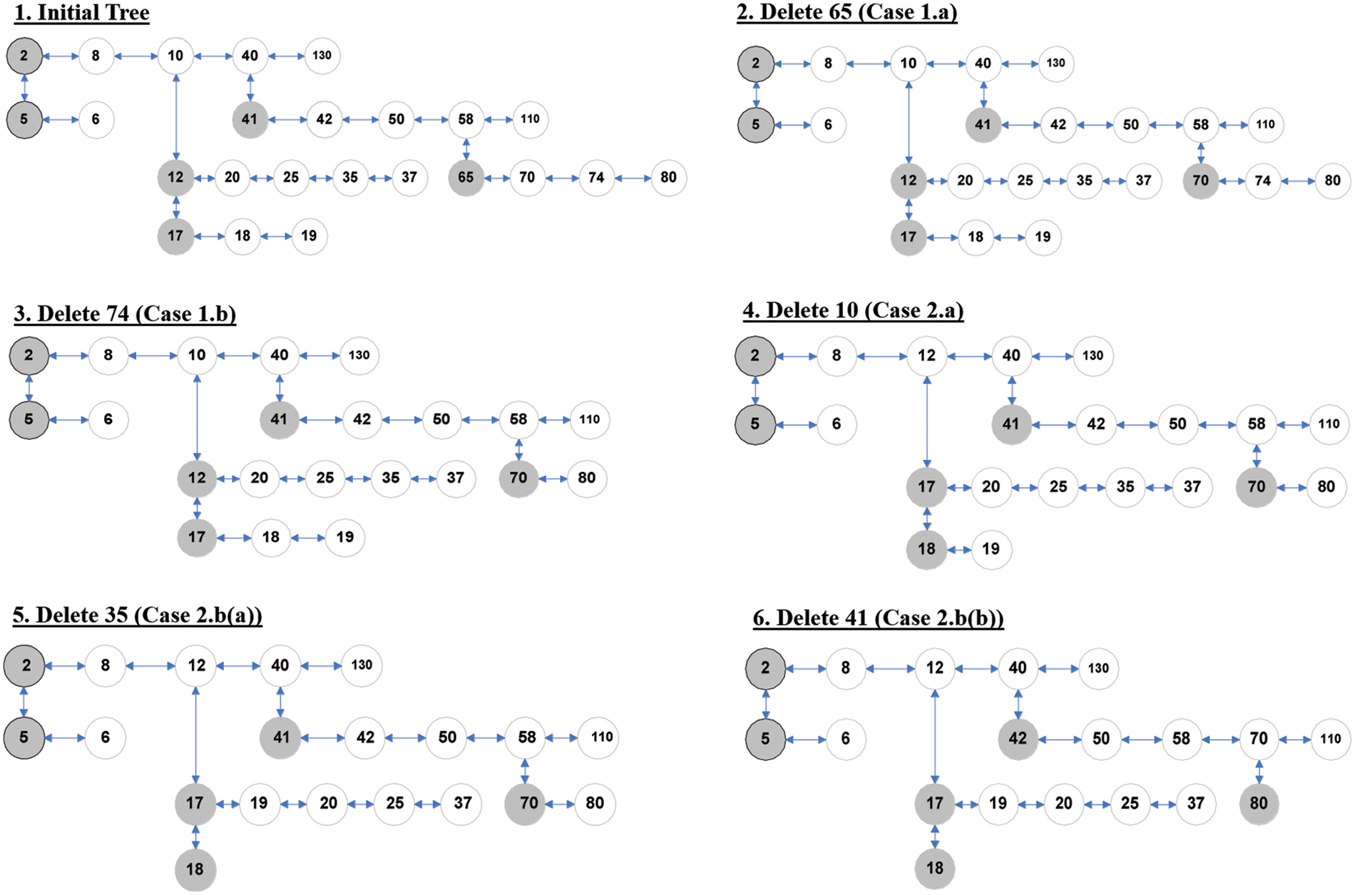
Figure 3: Various cases of deletion in OBLL

Step 5 in Fig. 3 depicts the case of deleting key 35. In this scenario, p starts pointing to the node with key element 35, and the mark node (nearest node of p with a child node, i.e., node with key element 17) is found to the left of p; as a result, the key elements from the next of mark are shifted to their right neighbor nodes until node p is found. The value of the last node of the mark node’s child list is then transferred to the next of mark node, and finally Delete_OBLL is called recursively on the last node of the mark node’s child list. Step 6 in Fig. 3 depicts the case of deleting key 41. In this case, p begins pointing to the node with key element 41. Node p is a member of a list that contains t nodes, and mark node is located on the right side of node p, therefore case 2.b(b) applies. As a result, until node p is discovered, the essential parts from mark node are moved to their left neighbors. The Delete_OBLL function is then executed recursively on the mark node. It’s case 2.a of the deletion method this time.

3.1.5 Traverse Operation

OBLL allows for faster traversal of its data components. In both situations (in-order and reverse order), the complexity of traversing the data comes out to be O(logtn).

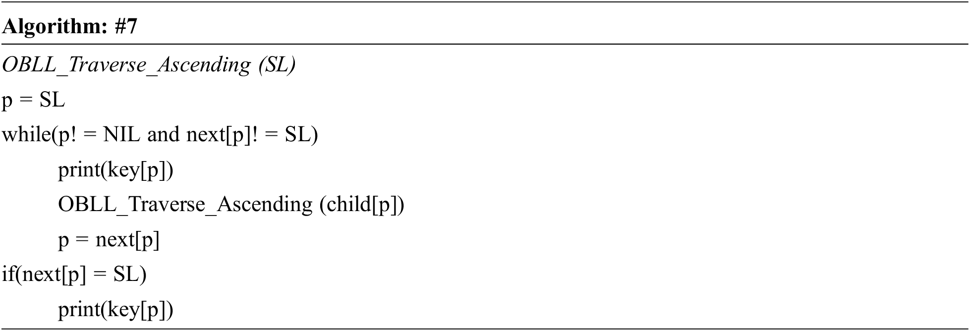
Traversing in the Increasing Order

OBLL use the recursive method the Algorithm #7 i.e., OBLL_Traverse_Ascending to explore the data in ascending order. This procedure takes one input argument, SL, which is the pointer to the current list’s start node. The algorithm prints the node’s key first, then proceeds down to the child of SL, calling OBLL_Traverse_Ascending on it repeatedly, and finally to the next node in SL.

Traversing in the Non-increasing Order

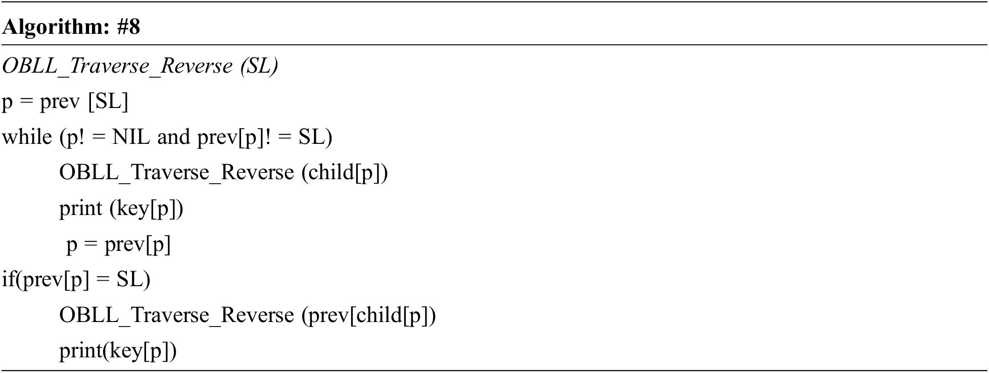
The Algorithm #8 i.e., OBLL_Traverse_Reverse is used to traverse data in a non-increasing order. OBLL_Traverse_Reverse is a recursive method that displays the key of SL (here SL points to the last node of the list, i.e., previous of the first node of a list), then goes down in SL’s child list, and lastly travels backward in the list.

3.2 Adopting OBLL for Conserving Energy

This study adopts the system model proposed in [18]. Accordingly, sinks may acquire historical information of certain mobile objects. Assuming the WSN is made up of identical sensors. Every sensor knows its surroundings and can identify movable objects inside its detection area. The surveillance region for the subject is partitioned into several grids. Every grid has a grid head that may encompass the whole grid and monitors activity occurrences in a continuous manner. The operational schedule of every node inside a grid is planned by a grid head, so that each sensor only works for a short duration and is powered off otherwise. Whenever a sensor node switches off, both its connection and sensing components are turned off. As per a specified hash algorithm or a random distribution, certain grid heads are picked as index nodes. Each grid head is aware of the index node to whom it relates. Sinks may submit query messages to the index node, which will then pass the information to the activity beginning point.

The information is dispersed on the monitoring node whenever the object travels randomly in the monitoring area. An OBLL is created in the suggested technique to assist the sink in getting past position data. A timestamp and link is coupled with this recorded activity whenever a sensor detects an activity. Every sensor will communicate its location as well as the time and date of the observed activity. Using overhearing, adjacent nodes will form a connection. Within the OBLL, a node’s next field stores the ID of the next sensor node, that stores the targeted object’s next location and data. Further, the node’s prev field reserves the ID of the sensor node that stores historic data and location of the roaming object.

Adopting OBLL to monitor item movement, users can conserve energy. Temporal data coupled by OBLL can clog up the cache of certain sensor nodes over a period. As a result, superfluous links lead the cache capacity to be depleted. In this case, cache space squandered, however redundant data often consumes virtually no power. Further, a mechanism is proposed to resolve the cache issue in [15]. However, adopting OBLL instead of standard linked list structure provides better efficiency as evaluated in next section.

4  Results

4.1 Proof of Correctness

To prove the correctness of OBLL we prove three lemmas.

Lemma 1. Order of OBLL structure can never be less than 3.

The OBLL order parameter is used to determine the maximum number of nodes in any OBLL list. The OBLL order is represented by the symbol t. To begin, if the value of t is set to 1, the whole OBLL structure will be a simple linked list, demonstrating the structure’s linearity. Second, if t is 2, the OBLL structure transforms into an unordered binary heap. In both instances, logarithmic time complexities are not attained in all cases of dynamic set operations.

Lemma 2. Last node of any list in OBLL does not have a child.

The data structure OBLL is framed under the idea of avoiding linearity in its structural design at any instant of dynamic set operation. This idea is subject to the constraint of OBLL property 4. Consider the scenario when the final node of the list is permitted to contain a child node; in this instance, the suggested OBLL will demonstrate linearity in its structure when values that are strictly increasing are inserted. Fig. 4 depicts the concept. When nodes are inserted with continually rising values of keys without the constraint of property 4, insertion of new node always takes as child node of the last node in the list, resulting in a linear structure that fails the OBLL concept.

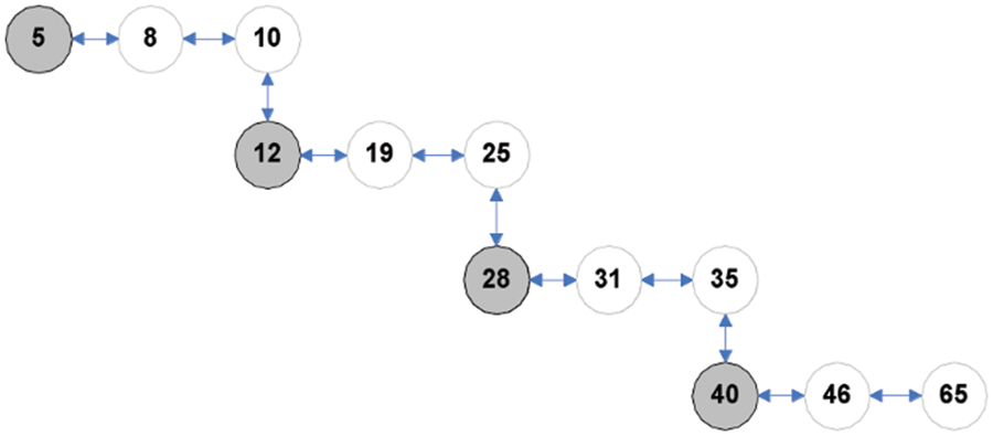
Figure 4: Violation of property 4

Lemma 3. OBLL works both as Min-Heap and Max-Heap.

Depending on the software application, frequent access to maximum and minimum components from the current data structure may be required. The max-heap or min-heap structures cannot meet this criterion of retrieving both the maximum and least element in a consistent time interval. Apart from heaps, the b-tree, which is often regarded as one of the greatest data structures for searching, fails to meet this criterion. Individually, searching for the largest and smallest element in a b-tree structure with n elements takes O (logtn) time. The main goal of the Max and Min heaps is to discover the structure’s maximum and minimal elements in a constant amount of time.

4.2 Simulation Results

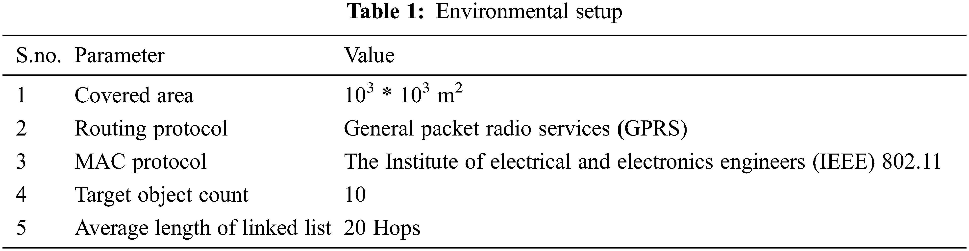
The current study simulates the network for experiment in Objective Modular Network Testbed in C++ (OMNET++) to evaluate the performance of adopting OBLL in place of EEDS proposed in [15]. Adopting exiting optimization of other parameters on the top of proposed method can result in better performance but authors in current research are restricting to perform evaluation on energy conservation through optimizing data storage only. However, authors aim to adopt such existing optimizations in near future. For the wide networks, EEDS is proved to be more energy efficient than External, internal, and data-oriented storage [15], thus we solely evaluated OBLL performance in comparison to EEDS. The simulation targets on overall energy usage in transmitting information, and query latency. The characteristics employed in OMNET++ simulations are listed in Tab. 1.

In certain applications, the WSN has a large number of sinks. It’s possible that the sinks will exit the WSN. Thus, the data from the departing sink must be transferred to other sinks. As a result, a handoff method is required to address this issue. As an outcome, messages are generated. Thus, experiments are conducted to observe the variation in transmitted messages. The simulation results are shown in Fig. 5, which illustrate the variation in the number of messages transmitted and the sensors present in network, which reflects energy cost. It can be observed that by using OBLL the number of messages transmitted is less than EEDS. The contributing factor behind this performance improvement is the low time complexity of data retrieval in OBLL. Further, it has been observed that the with a linear increase in the number of sensors, message count is also demonstrating a linear increasing behavior. However, the growth rate of message count in case of OBLL is less in comparison to EEDS.

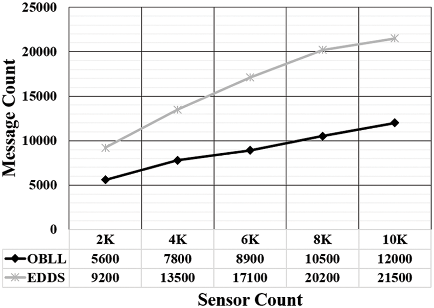
Figure 5: Variation in message transmitted

Since there is only one starting point in a general purpose linked list, all query operations should be sent to the linked list’s head node. This increases query latency and, as a result, energy consumption. Furthermore, if a linked list’s size is significant, the count of standby sensors should be sufficient to assure a successful retrieval. As a result, the current study conducted an experimental examination of the link between query latency and WSN sensors. The relationship between query latency and the sensors present in the network is seen in Fig. 6. It has been observed that OBLL has a better query latency over EEDS. The key factor for this performance behavior in OBLL is the low time complexity of data retrieval. Further, it has been spotted that the with a linear increase in the number of sensors, query latency is also increasing linearly. However, the growth rate of query latency in case of OBLL is less than that of EEDS.

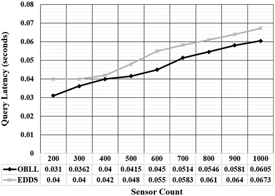
Figure 6: Query latency evaluation

The aggregate components of information that a system can handle in each time duration is referred to as throughput. Latency, on the other hand, is the time it takes for a system’s input to generate the intended response. Often, the channel itself contributes some latency in data transfer, which varies from one media to another. The volume of the packet transmitted per time leads to a delay, and a bigger packet takes more time to collect and deliver than a smaller one. The suggested system has been tested for query latency, and it has been shown to outperform the existing techniques. As a result, the suggested system has a high throughput for querying item tracking and determining object location.

4.3 Limitations and Future Work

In existing literature there are techniques that save energy optimizing various parameters of the WSN [28–30]. The current research targets to conserve energy through an optimized data storing approach to be used in WSN applications that require historical data related to monitor object activity. The current research doesn’t consider existing energy optimizations on parameters other than data storage. Thus, authors target to incorporate following existing energy optimizations techniques on the top of current research proposal in near future.

■   Authors aim to employ existing power optimizer scheduling techniques including HEEPS and GEDF [28] to achieve greater scheduling efficiency.

■   Authors aim to adopt various precautionary measures [29] to reduce energy consumption including optimal management system, prolonging the elapsed time between two neighboring occurrences, which could save detecting and interacting energy, and preferentially conveying findings, potentially saving interacting energy.

5  Conclusions

The storing technique of observed events affects the number of needed control messages in WSN. Because broadcasting unnecessary control messages wastes energy, reducing the number of control messages can increase the network’s lifespan. In this research, we present an energy conserving data storing approach that may be used in WSN applications that require historical data related to monitor object activity. The main concept is to create an Ordered Binary Linked List (OBLL) that follows the route of the desired object. The OBLL may be navigated with logarithmic complexity, which is significantly less than the traversing complexity of current linked list structures, to extract all the information. The simulation outcomes and performance analyses demonstrate that the proposed method does send fewer messages. Whenever the number of sensors in the system grows, the suggested technique surpasses existing approaches in the network.

Funding Statement: The authors received no specific funding for this study.

Conflicts of Interest: The authors declare that they have no conflicts of interest to report regarding the present study.

References

 1.  W. P. Chen, J. C. Hou and L. Sha, “Dynamic clustering for acoustic target tracking in wireless sensor networks,” IEEE Transactions on Mobile Computing, vol. 3, no. 3, pp. 258–271, 2004. [Google Scholar]

 2.  S. Ratnasamy, B. Karp, L. Yin, F. Yu, D. Estrin et al., “A geographic hash table for data-centric storage,” in The First ACM Int. Workshop on Wireless Sensor Networks and Applications (WSNA), Atlanta, Georgia, USA, pp. 78–87, 2002. [Google Scholar]

 3.  Y. C. Tseng, S. P. Kuo, H. W. Lee and C. F. Huang, “Location tracking in a wireless sensor network by mobile agents and its data fusion strategies,” The Computer Journal, vol. 47, no. 4, pp. 448–460, 2004. [Google Scholar]

 4.  G. Wang, J. Cao, H. Wang and M. Guo, “Polynomial regression for data gathering in environmental monitoring applications,” in IEEE GLOBECOM 2007 IEEE Global Telecommunications Conf., Washington, DC, USA, pp. 1307–1311, 2007. [Google Scholar]

 5.  S. Goel and T. Imielinski, “Prediction-based monitoring in sensor networks: Taking lessons from MPEG,” ACM SIGCOMM Computer Communication Review, vol. 31, no. 5, pp. 82–98, 2001. [Google Scholar]

 6.  E. Olule, G. Wang, M. Guo and M. Dong, “Rare: An energy-efficient target tracking protocol for wireless sensor networks,” in 2007 Int. Conf. on Parallel Processing Workshops (ICPPW 2007), Xi’an, China, pp. 76–76, 2007. [Google Scholar]

 7.  G. Wang, T. Wang, W. Jia, M. Guo and J. Li, “Adaptive location updates for mobile sinks in wireless sensor networks,” The Journal of Supercomputing, vo, vol. 47, no. 2, pp. 127–145, 2009. [Google Scholar]

 8.  Xu Y., Winter J., & Lee W. C. (2004). Prediction-based strategies for energy saving in object tracking sensor networks. In IEEE International Conference on Mobile Data Management, 2004. pp. 346–357. IEEE. [Google Scholar]

 9.  M. Bhardwaj and A. Ahalawat, “Improvement of lifespan of Ad hoc network with congestion control and magnetic resonance concept,” in Int. Conf. on Innovative Computing and Communications, Springer, Singapore pp. 123–133, 2019. [Google Scholar]

10. Y. Xu, J. Winter and W. C. Lee, “Dual prediction-based reporting for object tracking sensor networks,” in The First Annual Int. Conf. on Mobile and Ubiquitous Systems: Networking and Services, 2004. MOBIQUITOUS 2004, Boston, MA, USA, pp. 154–163, 2004. [Google Scholar]

11. W. Zhang and G. Cao, “DCTC: Dynamic convoy tree-based collaboration for target tracking in sensor networks,” IEEE Transactions on Wireless Communications, vol. 3, no. 5, pp. 1689–1701, 2004. [Google Scholar]

12. O. Nakov and D. Petrova, “Setting of moving object location with optimized tree structure,” in Proc. of the 11th WSEAS Int. Conf. on Computers, Stevens Point, Wisconsin, US, pp. 67–71, 2007. [Google Scholar]

13. J. Xu, X. Tang and W. C. Lee, “EASE: An energy-efficient in-network storage scheme for object tracking in sensor networks,” in 2005 Second Annual IEEE Communications Society Conf. on Sensor and Ad Hoc Communications and Networks, (IEEE SECON 2005), Santa Clara, CA, USA, pp. 396–405, 2005. [Google Scholar]

14. Y. Xu and W. C. Lee, “DTTC: Delay-tolerant trajectory compression for object tracking sensor networks,” in IEEE Int. Conf. on Sensor Networks, Ubiquitous, and Trustworthy Computing (SUTC’06), Taichung, Taiwan, vol. 1, pp. 8, 2006. [Google Scholar]

15. S. W. Ho and G. J. Yu, “An energy efficient data storage policy for object tracking wireless sensor network,” in IEEE Int. Conf. on Sensor Networks, Ubiquitous, and Trustworthy Computing (SUTC’06), Taichung, vol. 2, pp. 20–25. 2006. [Google Scholar]

16. C. R. Harris, K. J. Millman, S. J. van der Walt, R. Gommers, P. Virtanen et al., “Array programming with NumPy,” Nature, vol. 585, no. 7825, pp. 357–362, 2020. [Google Scholar]

17. W. Cai, H. Wen, H. A. Beadle, C. Kjellqvist, M. Hedayati et al., “Understanding and optimizing persistent memory allocation,” in Proc. of the 2020 ACM SIGPLAN Int. Symp. on Memory Management, New York, NY, United States, pp. 60–73, 2020. [Google Scholar]

18. K. Berney, H. Casanova, B. Karsin and N. Sitchinava, “Beyond binary search: Parallel in-place construction of implicit search tree layouts,” IEEE Transactions on Computers, 2021. vol. 71, pp. 1104–1116. [Google Scholar]

19. M. Long, Y. Li and F. Peng, “Dynamic provable data possession of multiple copies in cloud storage based on full-node of AVL tree,” International Journal of Digital Crime and Forensics, vol. 11, no. 1, pp. 126–137, 2019. [Google Scholar]

20. W. R. Arellano, P. A. Silva, M. F. Molina, S. Ronquillo and F. Ortega-Zamorano, “Red-black tree based NeuroEvolution of augmenting topologies,” in Int. Work-Conf. on Artificial Neural Networks, Springer, Cham, pp. 678–686. 2019. [Google Scholar]

21. M. Abdel-Basset, R. Mohamed, M. Elhoseny, R. K. Chakrabortty and M. J. Ryan, “An efficient heap-based optimization algorithm for parameters identification of proton exchange membrane fuel cells model: Analysis and case studies,” International Journal of Hydrogen Energy, vol. 46, no. 21, pp. 11908–11925, 2021. [Google Scholar]

22. Q. Askari, M. Saeed and I. Younas, “Heap-based optimizer inspired by corporate rank hierarchy for global optimization,” Expert Systems with Applications, vol. 161, pp. 1–27, article. 113702, 2020. [Google Scholar]

23. W. Ahmad, A. Rasool, A. R., Javed, T. Baker and Z. Jalil, “Cyber security in IoT-based cloud computing: A comprehensive survey,” Electronics, vol. 11, no. 1, pp. 16, 2021. [Google Scholar]

24. M. Majid, S. Habib, A. R. Javed, M. Rizwan, G. Srivastava et al., “Applications of wireless sensor networks and internet of things frameworks in the industry revolution 4.0: A systematic literature review,” Sensors, vol. 22, no. 6, pp. 2087, 2022. [Google Scholar]

25. S. R. K. Somayaji, M. Alazab, M. K. Manoj, A. Bucchiarone, C. L. Chowdhary et al., “A framework for prediction and storage of battery life in IoT devices using DNN and blockchain,” in 2020 IEEE Globecom Workshops (GC Wkshps), Madrid, Spain, pp. 1–6, 2020. [Google Scholar]

26. K. Dev, P. K. R. Maddikunta, T. R. Gadekallu, S. Bhattacharya, P. Hegde et al., “Energy optimization for green communication in IoT using harris hawks optimization,” IEEE Transactions on Green Communications and Networking, 2022. vol. 6, pp. 685–694. [Google Scholar]

27. A. K. Roy, K. Nath, G. Srivastava, T. R. Gadekallu and J. C. W. Lin, “Privacy preserving multi-party Key exchange protocol for wireless mesh networks,” Sensors, vol. 22, no. 5, pp. 1958, 2022. [Google Scholar]

28. R. Chéour, M. W. Jmal, S. Khriji, D. El Houssaini, C. Trigona et al., “Towards hybrid energy-efficient power management in wireless sensor networks,” Sensors, vol. 22, no. 1, pp. 301, 2021. [Google Scholar]

29. C. Pang, G. G. Xu, G. L. Shan and Y. P. Zhang, “A new energy efficient management approach for wireless sensor networks in target tracking,” Defence Technology, vol. 17, no. 3, pp. 932–947, 2021. [Google Scholar]

30. M. Bhardwaj, N. Shukla and A. Sharma, “Improvement and reduction of clustering overhead in mobile Ad Hoc network with optimum stable bunching algorithm,” Evolution of Software-Defined Networking Foundations for IoT and 5G Mobile Networks, IGI Global, vol. 1 pp. 139–158, 2021. [Google Scholar]