ELM-Based Shape Adaptive DCT Compression Technique for Underwater Image Compression

1  Introduction

Performance of underwater imagery system is influenced by channel characteristics like, limited bandwidth, blue/green lighting haze and noisy distortions due to lengthy cables between imaging device and storage device. Similarly, the transmission of underwater images under lower bandwidth and signal strength is a challenge and requires efficient compression techniques with minimum errors for reconstructed images or requires Spatial Modulation Schemes [1] for spectral and energy-efficient wireless communication systems. Compression techniques in underwater imaging offer the following attributes: lossy/lossless, quality scalability resolution scalability, Colour channel scalability, random access, Region of Interests (ROI)-based compression [2] etc. Several works represent that efficient compression techniques aids in tackling the limited bandwidth problem. In [3] proposed compression methods to divide the image database into tiles and approximation to get the reconstructed image. Another method of adaptive embedded coding compression on important regions was proposed [4] based on Image Activity Measurement (IAM) and Bits per pixel similarity (BPP-SSIM) curve method which is then used to predict the quality of image compression.

Another Adaptive method of Block Compression Sensing (BCS) was proposed [5]. The wavelet codec method and a preprocessing method are used to remove floating particles in underwater images [6]. Another work by [7] proposed wavelet-based preprocessing methods to remove visual redundancy by Wavelet Difference Reduction (WTWDR) and remove spatial redundancy in underwater ground images. In [8] proposed an intraframe coding technique for compression using spatiotemporal a noticeable distortion model to remove perceptual redundancy and uses motion interpolation to reduce the bit rate. In [9] proposed motion-compensated compression of underwater video imagery, where compression was achieved using the motion and radiometric information extracted from live and reconstructed images.

The above compression methods are block-wise compression techniques with fixed compression ratios or non-block-wise methods with different compression levels applied on the whole image. In recent years, there has been a lot of progress in several areas of learning technology, particularly image processing and computer vision. However, video compression learning is still in its infancy. This article looks at the collaborative work on learning for image and video codecs that has been ongoing for several years. For underwater images, a method of deriving saliency maps post veiling light removal and block-wise compression of regions by finding compression coefficients using an ELM-based network.

DCT is a straightforward transform technique. Some information is lost to compress an image. As a result, DCT classifies the spectral sub-bands of an image into the most significant frequency coefficients and the least important frequency coefficients. Environmental variables such as optical Noise, wave disturbances, light stability and equality, temperature changes, and other factors may all impact underwater photography quality, making underwater domain recording one of the most difficult undertakings. Various can use image processing techniques to process data and discover the best items and crucial features in pictures. Optical scattering is one of the primary difficulties in the underwater environment that can produce different distortions, including morphological change in the underwater image.

The benefit of getting DCT instead of Discrete Fourier Transform (DFT) is that it requires fewer total multiplications. When truncating frequency coefficients, DFT loses the form of the signal. Due to its continuous periodic characteristic, DCT preserves the form of the signal even after frequency coefficients are shortened. A concept for underwater photography, whether done by divers or with other specialist equipment However, most of the time, the image looked fuzzy. As a result, the image falls short of the viewers’ expectations. Certain processes must be carried out to get the image’s maximum perfection.

And the only multiplications involved in DCT are actual multiplications. Another benefit is that the lower frequency components store the majority of the signal energy compression. This characteristic of DCT arose from the image compression standards JPEG and MPEG. The undersea surface is a complex concept of image processes analysis. The surface has numerous aspects that make it more appealing than a terrestrial surface.

The Discrete Cosine Transform (DCT) breaks down a signal into its basic frequency components. It’s a popular image compression method. We create some basic methods to compute the DCT and compress pictures in this section. In all fields of digital signal processing, the Discrete Fourier Transform (DFT) is critical. It’s used in compression, filtering, and feature extraction to get a signal’s frequency-domain (spectral) representation. An image may be decomposed into its constituent parts using DCT.

Underwater imagery is a vital tool for documenting and reconstructing ecologically or historically significant locations that are inaccessible to the general public and scientific community. A range of technological and advanced equipment is utilized to get underwater imagery, including sonar, thermal imaging, an optical camera, and a laser. The discrete cosines transformation is widely used in image compression and video frame compression. This type of transformation will transfer a signal from the spatial domain to the time domain. DCT is suited for real-time applications because of its increased throughput. All Joint Photographic Experts Group (JPEG) image compression and Moving Picture Experts Group (MPEG) video compression formats. High-quality optical cameras are the preferred method for various computer vision tasks in contemporary underwater photography, covering from scene reconstruction and navigation to intervention tasks. However, processing underwater pictures and maintaining high levels of image quality might have some significant downsides.

2  Proposed Work

Underwater images suffer from veiling light which makes it very difficult to determine the ROI. Adding to veiling light, other factors that affect underwater image quality are color distortion, low contrast, blurriness, scattering effects and white color disbalancing, propagated light attenuation, and light scattering due to depth requires multiple repeated shots of the same object. The resulting underwater images have poor object boundaries making it difficult to recognize ROIs. This deeply affects the shape adaptive compression algorithms. As most shape adaptive compression techniques work on the saliency maps to detect the ROI, underwater image distortions give wrong saliency maps. This leads to the wrong estimation of the compression levels of objects of interest.

The first objective of this work is to restore the underwater color image of the veiling light to estimate the correct saliency values of the ROI. Another challenge in underwater sea picture imagery is the limited bandwidth of satellite/data uplinks which varies from place to place in the sea and weather. Hence compression levels to be applied on the ROI and rest of the region is dependent on the available bandwidth requires the computation of compression coefficient vis a vis input signal strength/bandwidth of channel transmitting the image and saliency value of the region. Several learning methods are available for the computation of compression coefficients. Still, most of them suffer from a typical problem like unsuitability when the target values overlap for given inputs, slow speed of learning network development, inability to expand the network when larger datasets arrive for training/testing, and the utmost prime issues like initializing the weights. To overcome this an ELM network is proposed to estimate the DCT coefficients. This reduces the training time and also, the hidden layers can be randomly assigned and is free from problems like finding local minima.

Fig. 1 shows the block diagram of the proposed work where the input image is restored from the blue/green light (veiling light affects). The fully compressed image is obtained by running the ELM-based DCT coefficient calculation for each image region. A saliency map was calculated for the underwater restored image and saliency value for the selected region R1. The available bandwidth or the signal strength was given to the ELM network to give the DCT coefficient values for the DCT based compression.

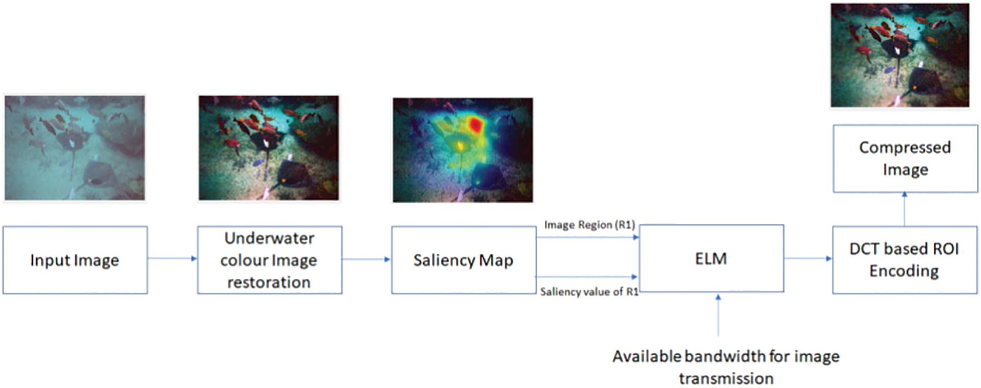
Figure 1: Block diagram of the proposed method

2.1 Underwater Color Image Restoration

Assuming an underwater camera, capturing the images in the deep sea with artificial lights. The use of artificial lights added to the veiling light components causes’ background scattering and also underwater floating particles generate unwanted noises and cause dimming of the captured images [10].

Any pixel coordinate (m, n) captured by the camera can thus be represented by a superposition model of direct energy transmission, forward scattering, and background scattering components represented by the equation below.

ET(m,n)=Ed(m,n)+Ef(m,n)+Eb(m,n) (1)

Here ET(m,n) is total energy component captured by the camera, Ed(m,n) is the direct energy transmission component, Ef(m,n) is the forward scattering component and Eb(m,n) is the backscattering component.

Image restoration techniques must recover the original image i(m,n) Schettini et al. 2010 [11] with minimum losses from an observed image o(m,n) while exploiting the degradation function d(m,n) and the noisy characteristics n(m,n) . The observed image thus is given by

o(m,n)=i(m,n)∗d(m,n)+n(m,n) (2)

Here * is the convolutional operator.

This can be represented in frequency domain by

O(u,v)=I(u,v)D(u,v)+N(u,v) (3)

where u, v are the spatial frequencies, O, I, D and N are the Fourier transform of o, i, d and n respectively. In image restoration techniques, where knowledge of degradation function or point spread function is required, it is very difficult to implement. In most conditions, a priori is not available and the point spread functions or the degradation models are tough to formulate for different depths of water. Occasional use of artificial light makes it difficult to formulate the same since uniform illumination cannot be assumed. Hence for image restoration it is important to incorporate underwater characteristics dependent on the depth of imagery into image restoration models.

An underwater color image is represented by three channels c ∈ {R, G, B}, and the intensity of each pixel is given by two components namely attenuated signal and veiling light Mao et al. 2014 [10].

Ic(x)=tc(x)Jc(x)+(1−tc(x)).Ac (4)

Here Ic is the captured image value in color channel c, the transmission of the particular color channel is given by tc . The scene value represents the global veiling light component where no objects are present and Jc is object radiance targeted to be restored.

The transmission depends on the objects distance d(x) and the water attenuation coefficient for each channel βc

tc(x)=exp⁡(−βcd(x)) (5)

Underwater imagery performed with the camera has three attenuation coefficients namely βR,βG,βB respectively, for the red, green and blue channels used for image restoration. To restore the color image and remove the underwater artifacts Dana et al. [12] methods of Veiling light Estimation and Transmission Estimation can be used as reference.

For transmission estimation of a particular channel, scene values can be used. The generalized scene values are given by

IChanel−I−channel=eβchannel(Ichannel−JChannel) (6)

Using Eq. (6) to calculate the ratio of attenuation coefficients between blue and red channels gives

(AR−IR)βBβR=e−βRd.βBβR(AR−JR)βBβR=tB(AR−JR)βBβR (7)

A lower bound on the transmission of the blue channel is given by

tLB:=max{1−IBAb,(1−IGAG)βBG,(1−IRAR)βBR} (8)

A soft matting method was used for calculating the transmission.

tB(x)={tLB(x)DM(I(x)≤DM+σMtBDM(I(x)≤DM+σMα(x)tLB(x)+1−α(x).t(x)otherwise (9)

where DM is the mahalanobis distance of the veiling light pixels given by

DM¯=1|VL|∑x∈VL⁡DMI(x) (10)

α(x) is the matting coefficient and σM is the standard deviation. After transmission estimation, scene recovery can be given by

Jc=Ac+Ic−Ace−βcd=Ac+Ic−ActBβcβB (11)

Overall the method involves the following steps:

1.    Detection of veiling light pixels using structured edges and calculation of veiling light A.

2.    The ratio of attenuation coefficients of Blue/Red and Blue/Green water type calculates the image intensity at a particular pixel for each value.

3.    Cluster the pixels into 500 Haze lines and estimate the initial transmission.

4.    Apply soft matting.

5.    Regularization using guided image filter with contrast-enhanced input as guidance.

6.    Calculate the Restored image.

7.    Return the image that best adheres to the Gray world assumptions.

2.2 Saliency Map

Saliency maps efficiently provide the Regions where most of the activity or objects of importance are present. Saliency maps effectively find the Region of Interest and are known to be used in several image segmentation problems to detect the salient visual regions. Several methods were proposed earlier for detecting saliency maps. Yang et al. [13] proposed color image-based saliency map derivation for foreign fiber detection by finding a color difference between pixel intensity and mean color value. Squaring this difference gave the mean value of color. Multitask Densely connected Neural Network (MDNN) was used to derive both salient maps and salient object subtilizing by Pei et al. [14]. Fast Fuzzy C means clustering algorithm with self-tuning local spatial information was used by Feng [15]. Self-attention-based saliency was used by Sun et al. [16] to generate a subtle saliency map. Another method of using multiscale image features were combined into a single topographical saliency map by Itti et al. [17]. A dynamical neural network then selects attended locations in order of decreasing saliency.

Saliency maps can be derived from single scale (properties) or multiple scales by adding two or more feature characteristics in deriving the saliency maps. There are various methods to determine saliency based on color, contrast, illumination etc. Most of the methods use the local contrast as one of the parameters for saliency map calculation. Feature vectors of a group of pixels for a particular region can be compared with feature vectors of the group of pixels for another region.

Split the image into 8 × 8 regions and calculate the GLCM features such as Regional contrast, Regional correlation and Entropy. GLCM features are normalized so that some of its elements are 1.

2.2.1 Entropy Calculation

Let (i, j) be the pixel coordinate of an image region R1. Assume GL to be the number of grey levels and Pk to be the probability associated with grey level k. The Entropy of a region R1 can be calculated [18] by

ER1=−∑k⁡pklog2(p2) (12)

2.2.2 Contrast Extraction

Contrast [19] returns a measure of the intensity contrast between a pixel and its neighbour over the whole image

CR1=∑i,j⁡|i−j|2p(i,j) (13)

2.2.3 Correlation Extraction

Correlation measures how correlated a pixel is to its neigh boring pixel over the whole image and ranges between −1 to 1.

CrR1=(i−μi)(j−μj)p(i,j)σiσj (14)

The GLCM feature [20] for the region R1 can be given as

R1=[ER1,CR1,CrR1] (15)

Weighted Euclidean Distance can be used to determine if any GLCM feature of Region 1 and Region 2 represents ROI or is not part of the ROI. The Euclidean distance between the jth variable of a feature between Region 1 and Region 2 can be given as

EDRj1−Rj2=∑j=1J⁡(Rj1sj−Rj2sj)2 (16)

Here sj is the sample standard deviation of the jth variable. In this case j = 3.

2.3 Application of ELM

ELM models can be solved analytically comprising of a closed-form involving matrix multiplication and inversion. Hence learning process can be started without any iterative methods and is considered faster compared to other algorithm. A classical neural network regression and prediction algorithm use fixed activation functions and dynamic changes are very difficult to implement. ELMs structure is simple and learning can be faster with good generalized performance. The Single hidden Layer Feed forward Neural Network (SLFN) architecture is shown in Fig. 2.

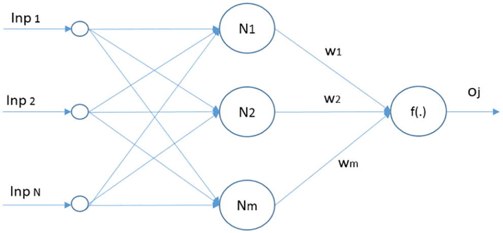
Figure 2: SLFN network architecture

Assuming N number of training samples (Inpi,ti)∈Rn×Rm(i=1,2,..N) . Output of the SLFN with N number of hidden nodes can be represented by

oj=∑i=1N⁡βifi(xj)=∑i=1N⁡βif(Inpj;ai,bi)j=1,...N (17)

Here oj is the output vector of SLFN concerning the input sample Inpj . Learning parameters are represented randomly by ai=[ai1,ai2,...ain]T and bi for the jth hidden node. The link connecting the jth hidden node and the output node is given by βi=[βi1,βi2,...βim]T . For the original ELM the activation function can be given by (Inpj;ai,bi) .

The inner product of ai,Inpj is given as ai,.Inpj . Output vectors can be presented as

Hβ=O (18)

H is the output matrix of the hidden layer. And illustratively represented as [21]

H=[f(a1.Inp1+b1)…f(aN.Inp1+bN)………f(a1.InpN+b1)…f(aN.InpN+bN)] (19)

β=[β1T…βNT]N×m (20)

O=[o1T…oNT]N×m (21)

The network cost function given as ||O-T|| can be minimized by assigning hidden node learning parameters without considering the input data, resulting in Hβ = O becoming a linear system and the output weights β is analytically determined by the least square method.

β^=H⊺T (22)

H⊺ is called Moore Penrose generalized inverse of H [22]. Hence, the calculation of the output weights is done by a mathematical transformation to avoid long training phases that involve adjusting the network iteratively with suitable learning parameters. ELM can be used to solve the regression problem where multiple inputs and a target set are used as in this case. The signal strength and saliency value of a block pixel are used as input training samples and the DCT coefficient output. Numerous functions are used for testing the regression problem.

f1(x)=∑i=1Dim⁡xi (23)

f2(x)=∑i=1Dim−1⁡100(xi−xi+1)2+(xi−1)2 (24)

f3(x)=−20e−0.2∑i=1mxi2Dim−e∑i=1n⁡cos⁡2πxiDim+20 (25)

Here Dim is the set of the positive integer representing the dimension of the function used. Function f2(x) and f3(x) are multimodal functions. The activation function is selected as a hyperbolic tangent function given by [23]

g(x)=(1−e−x)(1+e−x) (26)

For unbalanced learning, considering an N × N diagonal matrix W associated with every training sample Lp xi, the weight will be relatively higher than the others. To maximize the marginal distance and to minimize the cumulative error concerning the samples [24], ELMs can be optimized and written as

Minimise:‖Hβ−T‖2,‖β‖, (27)

Here T=[t1,,,tN]

Minimise:LPELM=12‖β‖2+12CW∑i=1N⁡‖ξi‖2 (28)

Subject to h(xi)β=tiT−ξiT,i=1,..N

Feature vector mapping in the hidden layer is represented by (Lp) xi concerning xi and the output vector connecting the hidden layer and output layer is represented by β . C represents a regularization parameter to represent the trade-off between the minimization of training errors and the maximization of the marginal distance ξi . The training error of sample xi is caused by the difference between the desired output ti and the actual output h(xi)β

ELMs come with their risks such as empirical and structural ones. A generalized ELM model must be able to balance and keep the empirical and structural risks at a minimum. But in cases where the input data results in overlapping of the target causes overfitting. Assuming input and output sample dataset for regression analysis as

T={(x1,y1),...(xi,yi)}

Here xi∈Rn and y∈R . Adjusting the proportion of the empirical and structural risk, the optimization model for the optimal regression can then by given by

min12‖β‖2+12ζ∑i=1N⁡‖δ‖2 (29)

Or Eq. (28) can be rewritten as

min12‖β‖2+12ζW∑i=1N⁡‖δ‖2 (30)

Subject to

{yi−βih(xi)=δiδi≥0,i=1,2..N (31)

As per the maximum margin theory t δi2 is the sum of the square errors representing the empirical risk and |β2| representing the structural risk.

Thus the overall steps involved in the ELM can be summarised as

■   Providing input training set, activation function f (.) and the number of hidden nodes.

■   Randomly assigning input weight w, input weight w and biases b.

■   Calculation of hidden layer output matrix H.

■   Calculation of output weight w.

Fig. 3 shows the flowchart of the ELM-based network in the proposed work. The first step involved defining the network parameters like activation function, the number of iterations, and the number of hidden neurons. ELM has the distinct advantage that weights and biases can be randomly assigned to the network. The next step is to train the ELM network with input as a training region saliency map for a region R1 and signal strength. Target DCT coefficients are set for the input and the training is done.

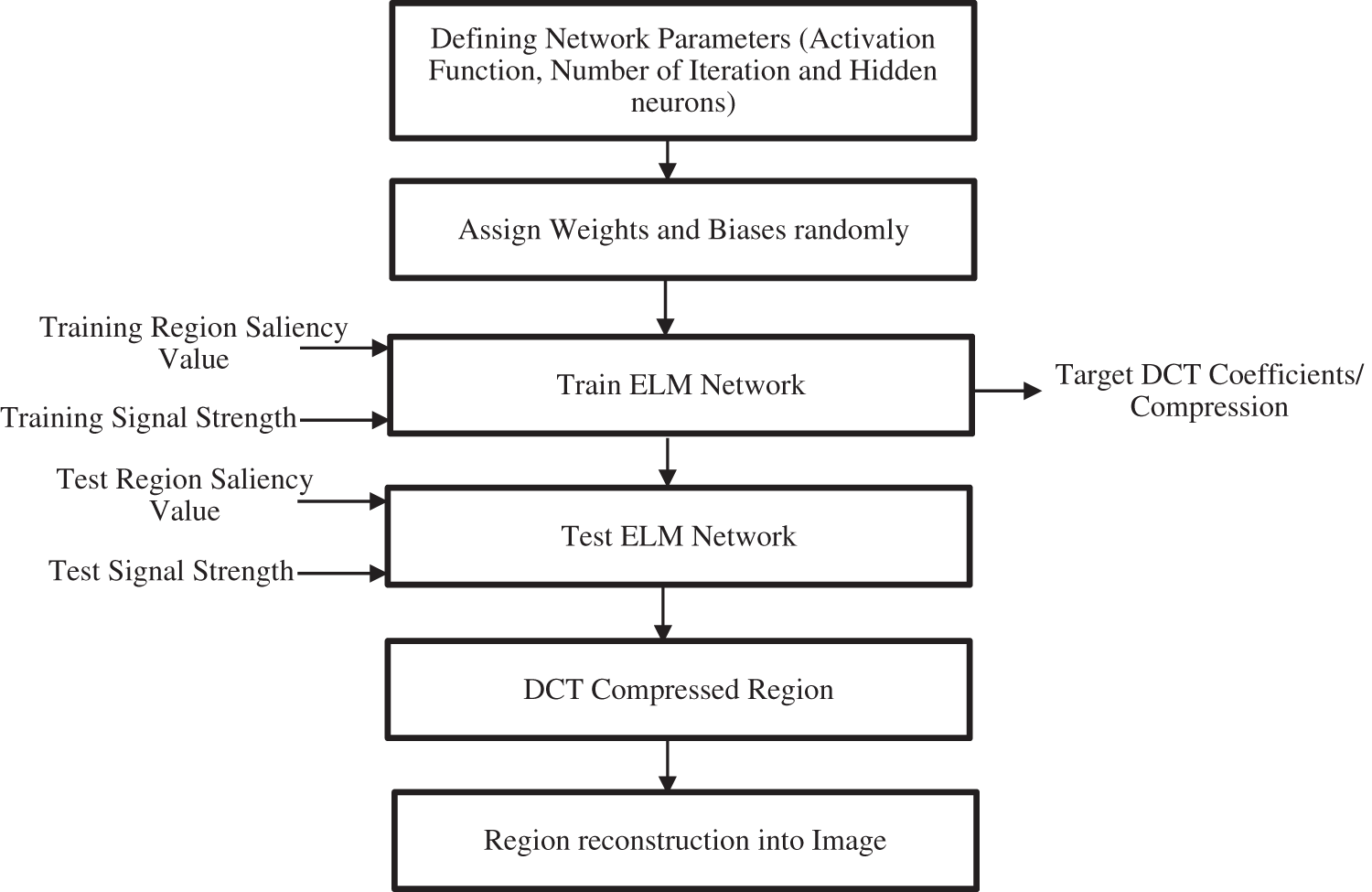
Figure 3: Flowchart for ELM-based training, and testing for compression of underwater images

To test the ELM network input Test Region Saliency values are given with the Test signal strength values. ELM network then estimates the correct output DCT coefficients/Compression Ratios. The coefficient is then selected for the region and the image is compressed for the region R1. The test process is done on the whole image while inputting image blocks to compress the whole image.

Although ELM is fast and gives good generalized performance since the output weights w and hidden biases are assigned randomly, some corner cases where ELM suffers from overfitting due to non-optimal input weights and hidden biases are present. To test the performance of the ELM RMSE is calculated.

RMSE=∑⁡Cof_Est_Erri2ni=1,2,3..n (32)

ME=∑Cof_Est_Errini=1,2,3..n (33)

Here Cof_Est_Err is the coefficient estimation error.

3  Results and Discussion

To test the algorithm, underwater marine images were taken. Fig. 4a represents an underwater image with a prominent blue light effect. Input image 4a is taken and a Saliency map is extracted as shown in 4c. A significant part of the ROI of the original underwater image is not given significant weights leading to a higher compression is adaptive shape methods in those areas where low compression levels should have been applied. Fig. 4e shows that higher compression levels were applied at even prominent ROIs, leading to a higher compression ratio and loss of ROI data during compression. To avoid this accurate saliency map extraction is important and the blue light effect must be removed. Underwater color image restoration was used to remove the blue/green light of the underwater marine images as shown in Figs. 4b–4d shows the saliency map of a restored color image from blue/green light effects and Fig. 4f shows the ELM-based shape adaptive DCT based compression. Same type of testing is applied for some more images and the results are shown in Figs. 5–9. The underwater color restored images have better PSNR and a lesser compression ratio to keep the quality of ROI significant.

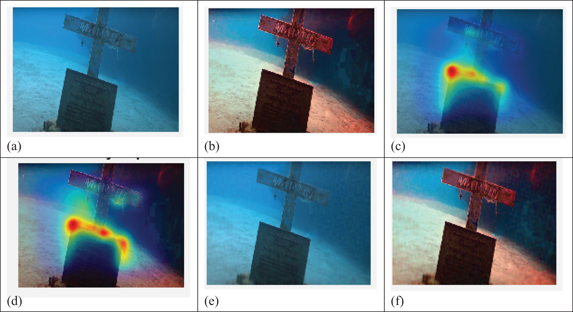
Figure 4: (a) Input image (b) Colour restored image (c) Saliency map for input image (d) Saliency map for Colour restored image (e) ELM shape adaptive DCT for input image: PSNR: 19.5, Compression Ratio: 20.22­­% (f) ELM shape adaptive DCT for color restored image: PSNR 28.2, Compression Ratio: 14.85

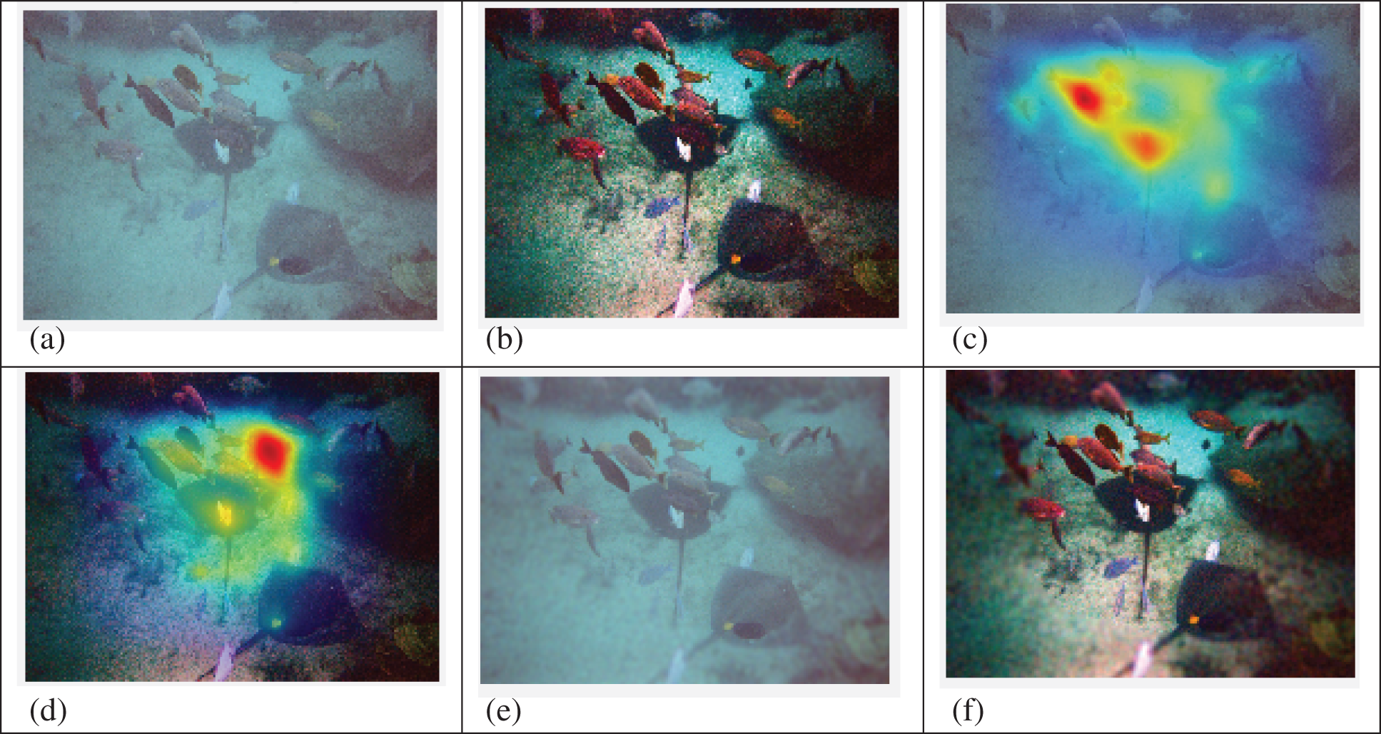
Figure 5: (a) Input image (b) Colour restored image (c) Saliency map for input image (d) Saliency map for Colour restored image (e) ELM shape adaptive DCT for input image PSNR:12.4 ,Compression Ratio: 17.58 (f) ELM shape adaptive DCT for colour restored image PSNR: 16.92, Compression Ratio: 16.25
Image Reference: http://labelme.csail.mit.edu/Release3.0/tool.html?actions https://=v&folder=users/antonio/static_sun_database/u/underwater/ocean_shallow&image=sun_bvoeqscrvbzdsaej.jpg

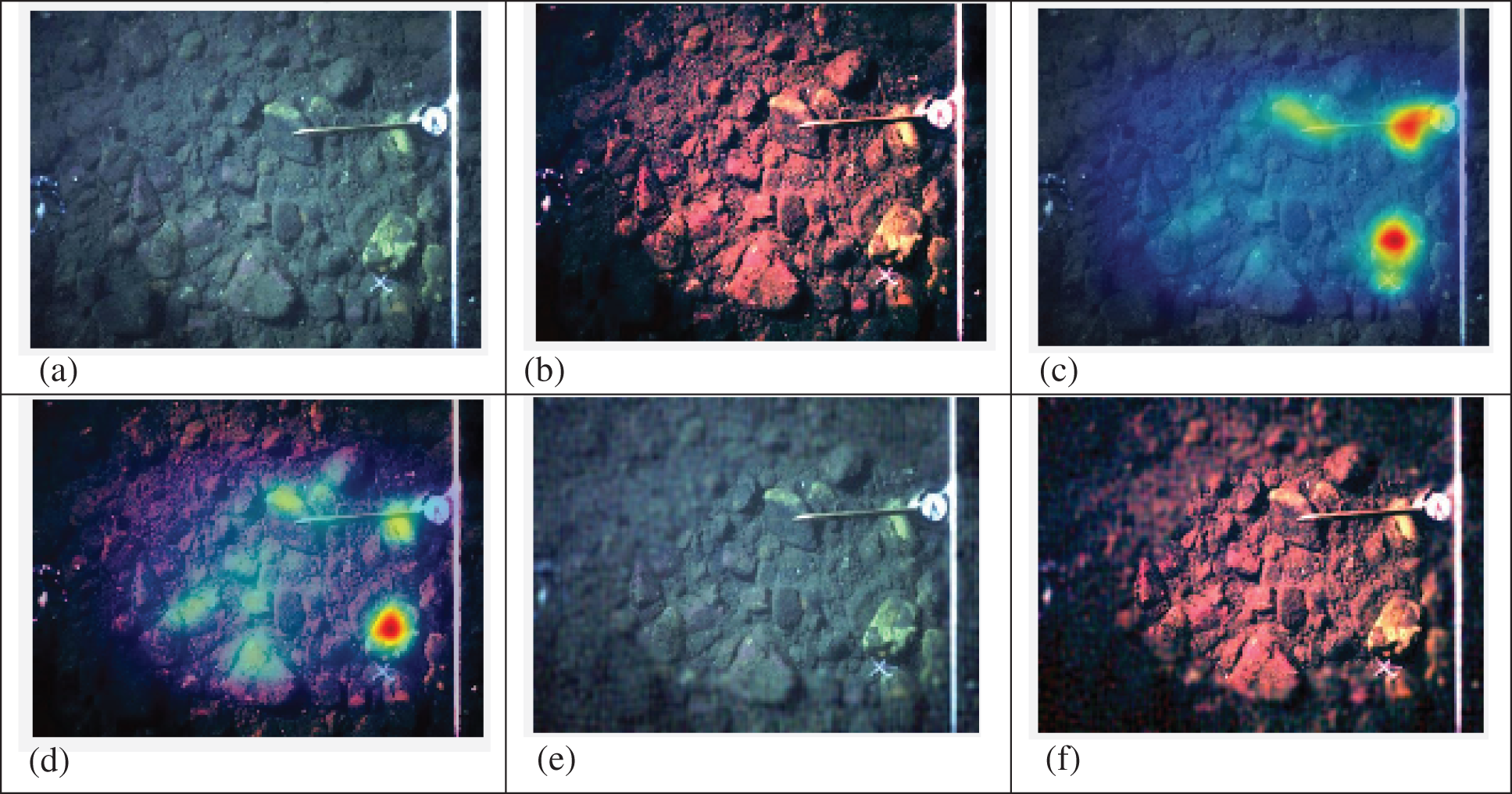
Figure 6: (a) Input image (b) Colour restored image (c) Saliency map for input image (d) Saliency map for Colour restored image (e) ELM shape adaptive DCT for input image PSNR:14.7, Compression Ratio: 23.69 (f) ELM shape adaptive DCT for colour restored image PSNR:16.78, Compression Ratio: 21.87
Image Reference: http://labelme.csail.mit.edu/Release3.0/Images/users/antonio/static_sun_database/u/underwater/ocean_shallow/sun_aqjzjtphfgrtgkyq.jpg

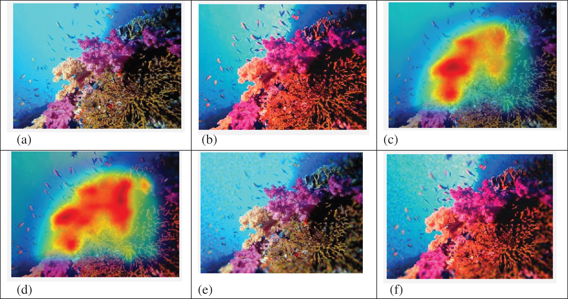
Figure 7: (a) Input image (b) Colour restored image (c) Saliency map for an input image (d) Saliency map for Colour restored image (e) ELM shape adaptive DCT for input image PSNR:21.24, Compression Ratio: 18.68 (f) ELM shape adaptive DCT for color restored image PSNR: 24.63, Compression Ratio: 14.58
Image Reference: http://labelme.csail.mit.edu/Release3.0/Images/users/antonio/static_sun_database/u/underwater/coral_reef/sun_bjmjisjcjszffzmo.jpg

Figure 8: (a) Input image (b) Colour restored image (c) Saliency map for input image (d) Saliency map for Colour restored image (e) ELM shape adaptive DCT for input image PSNR: 25.42, Compression Ratio: 21.23 (f) ELM shape adaptive DCT for color restored image PSNR: 28.72, Compression Ratio: 16.48
Image Reference: https://www.livescience.com/15492-underwater-shipwrecks-gallery.html

Figure 9: (a) Input image (b) Colour restored image (c) Saliency map for input image (d) Saliency map for Colour restored image (e) ELM shape adaptive DCT for input image PSNR:20.12, Compression Ratio: 21.26 (f) ELM shape adaptive DCT for colour restored image PSNR: 22.45, Compression Ratio: 17.68

After training the ELM for determining the DCT coefficients for the input of Saliency map value and signal strength for image transmission, the ELM network is tested. Fig. 10 shows that the compression applied to the input images goes down with the increase in the signal strength.

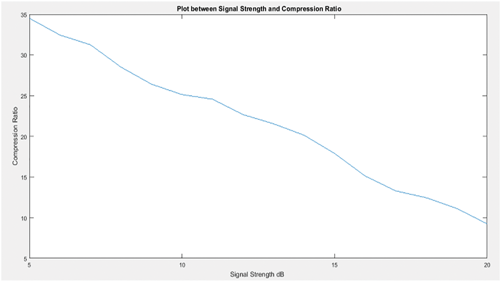
Figure 10: Plot between signal strength and compression ratio

Fig. 11 showed the PSNR values of one of the input images when the signal strength was varied across a range. With an increase in the signal strength, the PSNR also improves.

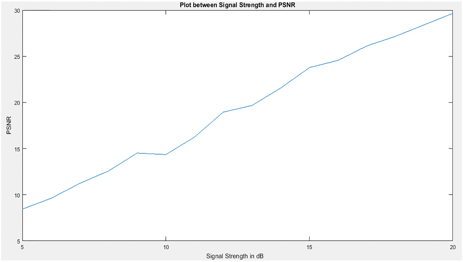
Figure 11: Plot between signal strength and PSNR

The Fig. 12 shows Structural content measures the image quality after degradation due to compression increases with an increase in the signal strength. Images get less degraded when the compression ratio is less when good signal strength is given to the system to transmit the images.

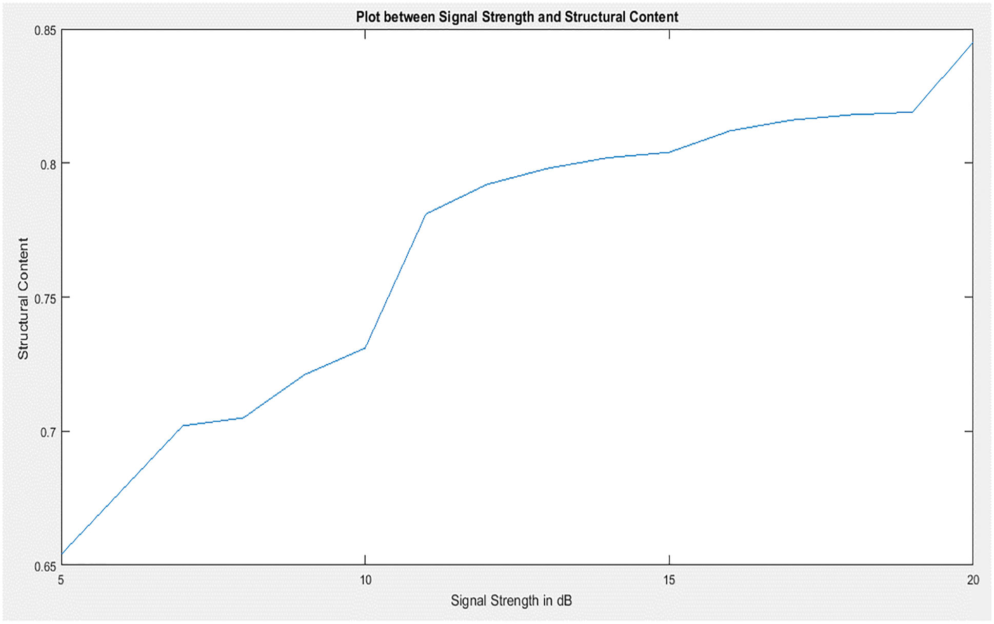
Figure 12: Plot between signal strength and structural content of MS-SSIM

With the decrease in the signal strength, the compression ratio has to be high, increasing the underground image’s processing timemage. Fig. 13 shows that processing time was higher when signal strength was decreased and as the signal strength improves processing time also improves for an image.

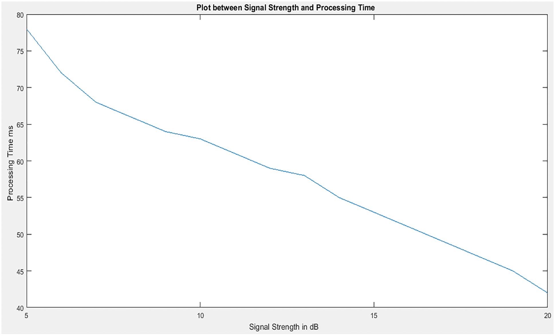
Figure 13: Plot between signal strength and processing time

Fig. 14 discuss the Plot between Signal Strength and Normalised Absolute Error. Normalized absolute error decreased with signal strength Normalized absolute error is higher when the signal strength is very low as there is a lot of error between the reconstructed and original images.

Figure 14: : Plot between signal strength and normalised absolute error

Fig. 15 discuss the comprehensive analysis of proposed system with some conventional methods. In this comparisons analysis clearly states the proposed ELM with DCT method gives good results.

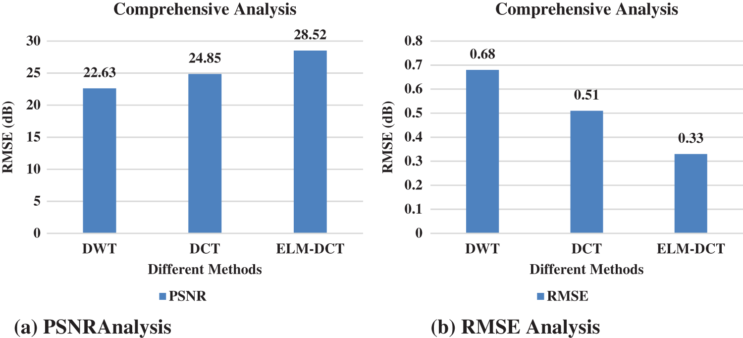
Figure 15: Comprehensive analysis

4  Conclusion

To handle the underwater image compression problem, this paper proposed a method that restores the underwater color image from the blue/green light rays and uses the saliency maps and signal strength to decide region level compression coefficients. Using ELM to find the compression coefficients proves itself efficient in providing optimal compression levels and PSNR values with minimized errors, minimized processing time and better structural content. The use of ELM resulted in a smaller processing time to set up the network as ELM has faster learning. The proposed method gives good results since the ELM reaches the solutions quickly without problems like local minima and learning rate. The PSNR and RMSE value of proposed system is 28.52 dB and 0.33 dB.

Funding Statement: The authors received no specific funding for this study.

Conflicts of Interest: The authors declare that they have no conflicts of interest to report regarding the present study.

References

1. H. Esmaiel, Z. A. H. Qasem, H. Sun, J. Wang, N. U. Rehman Junejo “Underwater image transmission using spatial modulation unequal error protection for internet of underwater things,” Sensors, vol. 9, no. 23, pp. 5271, 2019. [Google Scholar]
2. M. Eduardo, D. Centelles, J. Sales, J. Vte and M. R. N. Pedro et al., “Wireless image compression and transmission for underwater robotic applications,” IFAC-Papers on Line, vol. 48, no. 2, pp. 288–293, 2015. [Google Scholar]
3. B. Sánchez, P. Papaelias, G. Márquez and F. Pedro, “Autonomous underwater vehicles: Instrumentation and measurements,” IEEE Instrumentation & Measurement Magazine, vol. 23, pp. 105–114, 2020. [Google Scholar]
4. Y. Cai, H. X. Zou and F. Yuan, “Adaptive compression method for underwater images based on perceived quality estimation,” Frontiers of Information Technology & Electronic Engineering, vol. 20, pp. 716–730, 2019. [Google Scholar]
5. W. Chen, F. Yuan and E. Cheng, “Adaptive underwater image compression with high robustness based on compressed sensing,” in IEEE Int. Conf. on Signal Processing, Communications and Computing (ICSPCC), Hong Kong, China, pp. 1–6, 2016. [Google Scholar]
6. D. H. Kim and J. Y. Son, “Underwater image pre-processing and compression for efficient underwater searches and ultrasonic communications,” International Journal of Precision Engineering and Manufacturing, vol. 8, No.no. 1, pp. 38–45, 2017. [Google Scholar]
7. Q. Z. Li and W. J. Wang, “Low-bit-rate coding of underwater color images using improved wavelet difference reduction,” Journal of Visual Communication and Image Representation, vol. 21, no. 7, pp. 762–769, 2010. [Google Scholar]
8. Y. Zhang, S. Negahdaripour and Q. Li, “Low bit-rate compression of underwater imagery based on adaptive hybrid wavelets and directional filter banks,” Signal Processing: Image Communication, vol. 47, pp. 96–114, 2016. [Google Scholar]
9. S. Negahdaripour and A. Khamene, “Motion-based compression of underwater video imagery for the operations of unmanned submersible vehicles,” Computer Vision and Image Understanding, vol. 79, no. 1, pp. 162–183, 2000. [Google Scholar]
10. L. Mao, L. Zhang, X. Liu, C. Li and H. Yang, “Improved extreme learning machine and its application in image quality assessment,” Hindawi Publishing Corporation Mathematical Problems in Engineering, vol. 2014, no. 426152, pp. 1–7, 2014. [Google Scholar]
11. R. Schettini and S. Corchs, “Underwater image processing: State of the Art of restoration and image enhancement methods,” EURASIP Journal on Advances in Signal Processing, vol. 2010, no. 746052, pp. 1–14, 2010. [Google Scholar]
12. M. Dana, T. Tali and S. Avidan. “Diving into haze-lines: Colour restoration of underwater images,” in British Machine Vision Conf. (BMVC), London, pp. 1–12, 2017. [Google Scholar]
13. W. Yang, D. Li, S. Wang, S. Lu and J. Yang, “Saliency-based colour image segmentation in foreign fiber detection,” Mathematical and Computer Modelling, vol. 58, no. 3–4, pp. 852–858, 2013. [Google Scholar]
14. J. Pei, H. Tang, C. Liu and C. Chen, “Salient instance segmentation via subitizing and clustering,” Neurob Computing, vol. 402, pp. 423–436, 2020. [Google Scholar]
15. Z. feng, “Fuzzy clustering algorithms with self-tuning non-local spatial information for image segmentation,” Neuro Computing, vol. 106, pp. 115–125, 2013. [Google Scholar]
16. F. Sun and W. Li, “Saliency guided deep network for weakly-supervised image segmentation,” Pattern Recognition Letters, vol. 120, pp. 62–68, 2019. [Google Scholar]
17. L. Itti, C. Koch and E. Niebur, “A model of saliency-based visual attention for rapid scene analysis,” IEEE Transactions on Pattern Analysis and Machine Intelligence, vol. 20, no. 11, pp. 1254–1259, 1998. [Google Scholar]
18. Y. Yoav and N. Karpel, “Recovery of underwater visibility and structure by polarization analysis,” IEEE J, Oceanic Engineering, vol. 30, no. 3, pp. 570–587, 2005. [Google Scholar]
19. C. B. Honeycutt and R. Plotnick, “Image analysis techniques and gray-level co-occurrence matrices (GLCM) calculate bioturbation indices and characterize biogenic sedimentary structures,” Computers & Geosciences, vol. 34, no. 11, pp. 1461–1472, 2008. [Google Scholar]
20. X. Zhang, X. Liu and Q. Yu, “Comparative high contrast area extraction in image based on spatial-contrast feature,” in Int. Conf. on Computer Graphics, Imaging and Visualization (CGIV’05), Beijing, China, pp. 133–136, 2005. [Google Scholar]
21. R. Priyanka and D. Kumar, “Feature extraction and selection of kidney ultrasound images using GLCM and PCA,” Procedia Computer Science, vol. 167, pp. 1722–1731, 2020. [Google Scholar]
22. Q. F. Ertuğrul and Y. Kaya. “A detailed analysis on extreme learning machine and novel approaches based on ELM,” American Journal of Computer Science and Engineering, vol. 1, no. 5, pp. 43–50, 2014. [Google Scholar]
23. L. Shuxia, W. Xi-Zhao, Z. Guiqiang and Z. Xu, “Effective algorithms of the moore-penrose inverse matrices for extreme learning machine,” Intelligent Data Analysis, vol. 19, no. 4, pp. 743–760, 2015. [Google Scholar]
24. L. Chao and M. Wang, “Removal of water scattering,” in 2nd. Int. Conf. on Computer Engineering and Technology, Chengdu, vol. 2, pp. 35–39, 2010. [Google Scholar]
Cite This Article
Copyright © 2023 The Author(s). Published by Tech Science Press.
This work is licensed under a Creative Commons Attribution 4.0 International License , which permits unrestricted use, distribution, and reproduction in any medium, provided the original work is properly cited.
Downloads
Citation Tools