Radial Basis Approximations Based BEMD for Enhancement of Non-Uniform Illumination Images

1  Introduction

Now days, image processing has become a renowned area as it has a wide range of applications in almost all the areas. Image processing is used for feature extraction, medical imaging, face recognition, character recognition, finger print recognition, crime detection, painting restoration, microscope imaging etc. [1]. Image enhancement is an important area of image processing as it can help in other areas also to solve different purposes [2]. There can be many reasons for image degradation which makes it necessary to enhance the image. When an image is captured under improper illumination, it is known as non-uniform illumination image. It can hide some important information present and affect the visual quality of image [3]. These degradations make an image less suited for any application. Thus, image enhancements for non-uniform illumination image become necessary to get all details hidden under dark portions and to make the image more eyes soothing [4].

There exist many intensity transformation algorithms in literature which can be used for enhancement of non-uniform illumination images like log transformation, power law transformation, gamma correction transformation, dynamic range compression, histogram equalization etc. [5]. Log transformation converts the low intensity values to high intensity. Dynamic range compression is technique where ratio of the brightest and darkest intensity is compressed by using log transformation [6]. In gamma transformation, different enhancement level can be obtained for different values of gamma [7]. Histogram equalization is a technique used to get the contrast enhanced image by adjustment of the intensity level present in given image [8].

Alpha rooting is another method for image enhancement. It does enhancement in spatial domain as well as frequency domain. It is used to make the high frequency details present in an image more noticeable by using power law or log transformation method for mapping the narrow gray level range to wider range. This method provides good contrast and detailed image [9].

Jobson et al. proposed Retinex algorithm for image enhancement. According to Retinex theory, an image is a combination of illumination and reflectance [10,11]. On the basis of Retinex theory, SSR (Single Scale Retinex) [12] and MSR (Multi Scale Retinex) [13] algorithms were given for enhancement of non-uniform illumination image. Both these algorithm gives reflectance as the enhanced image but causes halo artifact which makes bright portion of image brighter [14]. To eliminate this artifact, MSRCR (Multi Scale Retinex with Color Restoration) algorithm was proposed which restores the color of enhanced image and thus makes an image more eye soothing [15].

DCT (Discrete Cosine Transformation) based algorithm for image enhancement was proposed by S. Mitra for the enhancement of non-uniform illumination images [16]. This algorithm preserves the local contrast of image and enhances background illumination by scaling the DC coefficients of image. This algorithm works in compressed domain which minimizes the computation complexity [17].

Another method for enhancement of low light images is fusion based methods. This method deals with the process of capturing many images of the same scene by using either different sensors or by the same sensors at different times. Enhancement based on multi-spectrum-based fusion involves the fusion of original low light image with Infrared image (IR) or with Near IR image [18,19].

Choi et al. proposed another algorithm for enhancement of non-uniform illumination images known as JND (Just Noticeable Difference) nonlinear filter-based enhancement [20]. In this, the illumination is extracted by using the JND based non-linear filter [21] and saturation part is enhanced in accordance to enhanced intensity component [22].

Since all the existing algorithms in literature do not preserve the natural colour of image. Also, there is a compromise between the naturalness and the information present in an image. This gives the need for an algorithm which not only enhance the information content present in image but also gives the more eye soothing enhanced image along with naturalness preservation. To meet these requirements, a new algorithm has been proposed in this paper for the enhancement of non-uniform illumination images in which Bi-dimensional empirical mode decomposition-based enhancement is performed on intensity component along with saturation component.

2  EMD (Empirical Mode Decomposition)

Non-stationary and non-linearity basically means that data is available non-linearly or it is linear for short time periods [23]. Analysis of such kind of data is not simple as that of analysis of linear and stationary data. To find a solution for this kind of data is very important for solving the many real-life phenomena. Spectrogram, discovered by G. Kratzenstein, is the basic technique used for given non-linear data. It basically analyzes the data using Fourier transform for limited time scale. On sliding the window on given data, analysis can be done but this technique was not efficient one because it is not guaranteed that the data available for particular window size will be stationary only or what will be the window size that can be taken for particular time span. So, an efficient method was needed for analysis of such kind of data [24].

Empirical mode decomposition-based data analysis was discovered by N. Huang in 1998. Such kind of data can be analyzed using the Hilbert transform by which instantaneous frequency can be determined corresponding to the different modes present at different intrinsic time spans [25]. On applying the Hilbert transform to the modes obtained on decomposing the original data, instantaneous frequency can be calculated but there are some restrictions on this frequency. The instantaneous frequency can be determined only when the given data will be symmetric locally across the zero-mean level [26]. This restriction imposed on instantaneous frequency give rise to a class of function based on its local properties known as IMF (Intrinsic Mode Function). So, in EMD, the decomposition of given non-linear data set is performed to get various intrinsic mode functions representing the different modes of oscillation. The obtained intrinsic mode functions must follow the property of completeness and orthogonally [27].

2.1 IMF

IMF’s represent different modes present in an image. There are certain conditions to be satisfied for any function become an IMF. The total count of local maxima, local minima and zero crossing present in any IMF must be either equal or differ by almost one unit. Local maxima and minima refer to the highest and lowest notches present in different waves present in an IMF. The local mean value of the envelopes made by local maxima and local minima at any point must be zero. Here local mean of the data should be used but for non-linear data it is very difficult to represent any local time scale. So, the mentioned envelope local mean is formed by taking local minima and maxima into account [28].

2.2 Sifting Algorithm for Mode Decomposition

Whenever at a particular time, various oscillatory modes are present in the data; the analysis of such kind of data can be done by decomposing it into various modes corresponding to intrinsic time span. Sifting algorithm is used for this decomposition of the original data [29]. During the decomposition, intrinsic oscillatory modes are identified according to their time scales in the data and then decomposition process occurred.

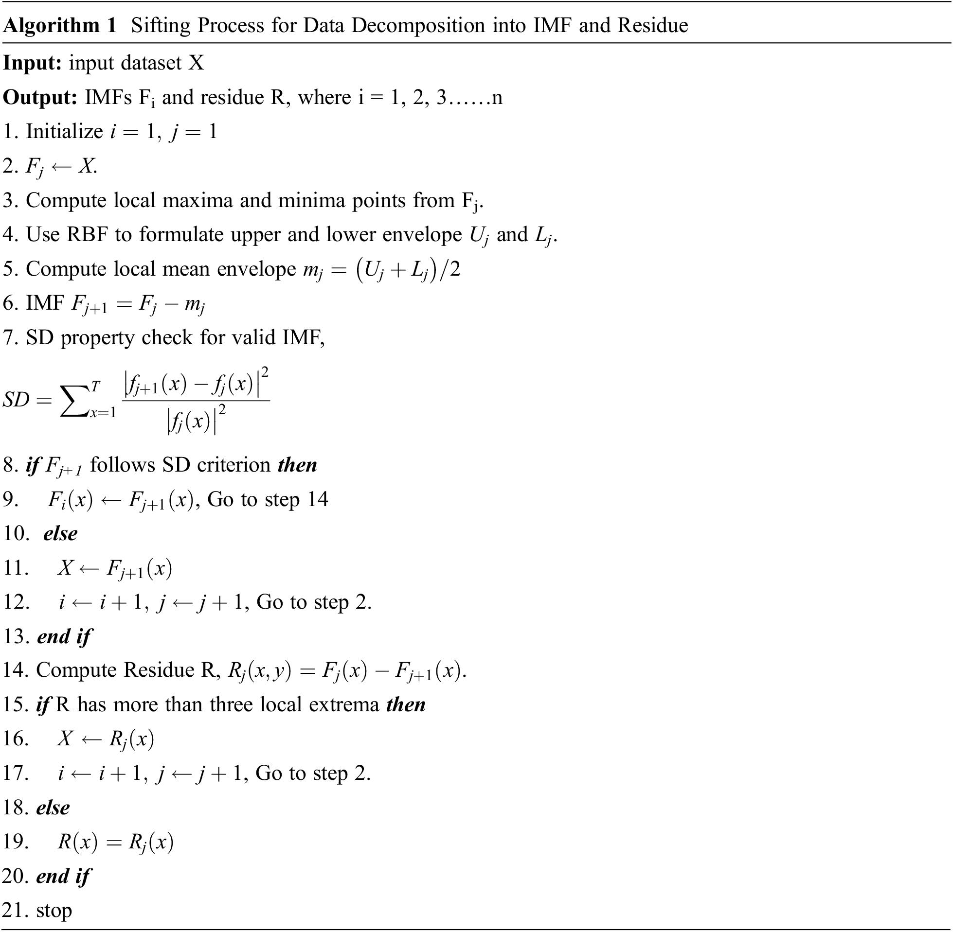
In the sifting process, given data is taken as input z(t). The local maxima and local minima are calculated from the given data by using the windowing method all across the length of data set. Next, the surface reconstruction is carried out to obtain the upper and lower envelope by using any interpolation technique [30]. In the proposed algorithm, radial basis approximation-based interpolation technique is used to construct the envelopes from local minima and maxima points. The choice of interpolation technique matters a lot as it decides the quality of intrinsic mode functions obtained. The process of sifting algorithm for mode decomposition is represented by algorithm 1. There are two ways to stop the sifting process. First, it may depend on our choice that how many IMFs we are interested in or the process can be stopped on a well-defined criterion which is given by standard deviation represented as follows:

SD=∑t=0T|fpresent(t)−fprevious(t)|2|fprevious(t)|2 (1)

The standard deviation value should be between 0.2 and 0.3, whenever the standard deviation will be less than the given threshold value, the sifting process is stopped and IMF will be obtained. On continuing this process, when the situation occurs where residue will act like a monotonic function then this sifting process will terminate and IMFs and residue corresponding to given input data will be obtained [31]. The original data can be obtained as shown as follows:

z(t)=∑t=0Tfi+rn (2)

According to decomposition theory, all the IMFs should be orthogonal to each other. The overall index of orthogonally can be obtained by using the expression given below.

OI=∑t=0T(∑j=1n+1∑k=1n+1fj(t)fk(t)z2(t)) (3)

`Here (n + 1)th notation is used to represent the residue obtained. Lower the value of orthogonally, better will be the IMF decomposition [32,33].

3  Radial Basis Approximation Based Interpolation

Scattered data or random data can be interpolated by using the radial basis approximations. After calculating the local extreme, upper and lower envelope can be constructed by using radial basis function [34]. This function is a real valued function which basically depends on the distance of a point from another point which acts as the center. Suppose the given data set is denoted by D∈(xi,yi) . The target result is affected by the distance which is the calculated by the norm between the two data points which acts as the basis function for radial basis function and can be represented as ϕ‖(x−xI)‖ . The point in the given data set will affect the nearby point compare to the far away point. This is the main component of the radial basis function. The standard form of radial basis function is given as follows:

F(x)=∑i=0Nwiϕ‖(x−xI)‖ (4)

where xi and x represents the location of known nodes and point at which the value of function is to be calculated. The main aim of the radial basis approximation is to calculate a mapping function which can map efficiently the given input data set to the given output data set which error as low as possible. So, according to formula written above, radial basis function is the linear weighted summation of the various basis functions which lies at different centers for a given point at which value of F(x) is to be evaluated [35]. So, Eq. (4) can be modeled as follows:

F(xj)=∑i=1mwiϕ‖(xj−xI)‖,j=1,2,3,….,N (5)

A first degree polynomial needs to be added for linear and constant portion of F which is represented as follows:

F(xj)=∑i=1mwiϕ‖(xj−xI)‖+P(x),j=1,2,3,….,N (6)

where xI are the N points at which function, value is to be calculated and xi works as the center of each basis function. The function should be approximated in such a way that it will exactly equal to output data points corresponding to input data points which acts as a constraint and is expressed as follows:

F(xj)=∑i=1mwiϕ‖(xj−xI)‖+P(x)=yj (7)

where, yj are the output points. Matrix form can be obtained by expanding the above expression represented as follows:

[Φ11ϕ21...ϕn1C1xC1y1ϕ12ϕ22...ϕn2C2xC2y1...........................ϕ1nϕ2n...ϕnnCnxCny1C1xC2x...Cnx000C1yC2y...Cny000C1zC2z...Cnz00011...1000][w1w2...wnγxγyγz1]=[y1y2...yn0000] (8)

where, ϕji=ϕ‖(xj−xi)‖ can be modelled as interpolation matrix. The above matrix can be represented as follows:

ϕjiwi=yj (9)

where ϕji is a function of xj and xi and (j,i) ∈ 1, 2, 3…N. Solution to the above-mentioned expression has to be done for estimating the radial basis coefficients which can be further used for

interpolating the desired surface. Weights values can be estimated only when interpolating matrix will be a non-singular matrix for its inevitability property. Certain radial basis functions like Gaussian basis function, cubic, thin-plate, linear and multi-quadratic have been proved good for interpolation. These functions will always give a non-singular interpolation matrix. The radial basis functions for the thin plate model are being used in the proposed algorithm expressed below:

Φ(r)=r2logr (10)

Solving the above expression RBF coefficients can be calculated by the following expression:

wi=Φ−1yj (11)

where wj are RBF coefficients or weights obtained. Finally surface interpolation can be done by implementing the following expression:

F(x)=C0+C1x+∑i=1Nwiϕ‖(x−xi)‖ (12)

where C0 and C1 are radial basis coefficients calculated by adding the polynomial term [36].

4  Two Dimensional EMD

The 2-Dimensional EMD process is known as bi-dimensional empirical mode decomposition. The analysis of an image can be done in a better way by analyzing its IMFs as compare to full image [37].

This technique is popular in various image fields as it can be used for image fusion, image de-noising, analysis image enhancement, texture analysis, medical imaging etc. This technique uses the sifting process discussed in algorithm 1 for decomposition of given image into high frequency and low frequency Intrinsic mode functions. The high frequency IMFs represents the details present in the image and the residue or low frequency IMF has the lightness information of the image [38,39].

Fig. 1 represents interpolation process using radial basis apprximations and Fig. 2 represents bi-dimensional empirical mode decomposition results of an image into BIMFs and a residue in which various BIMFs contain the details of the image and residue part contains the lightness information. Fig. 2a represents the original image of satellite view captured from a certain height in which due to improper lightening the scene has become dull and actual colors present in image are hidden. Figs. 2b to 2e represents three BIMFs and residue. It can be noticed that as the decomposition proceeded, amount of information or details becomes smaller in the BIMFs. Fig. 2b which is high frequency component is high in details and Fig. 2c is second BIMF component, which contains information but details become less. Similarly, Fig. 2d represents the image which contains very few information and Fig. 2e represents the final residue which shows the lightness information. So, it is clear that details are preserved in high frequency components which are named as intrinsic mode functions and lightness information is preserved into the residual component.

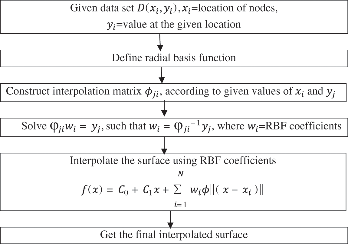
Figure 1: Block diagram of interpolation process using radial basis approximations

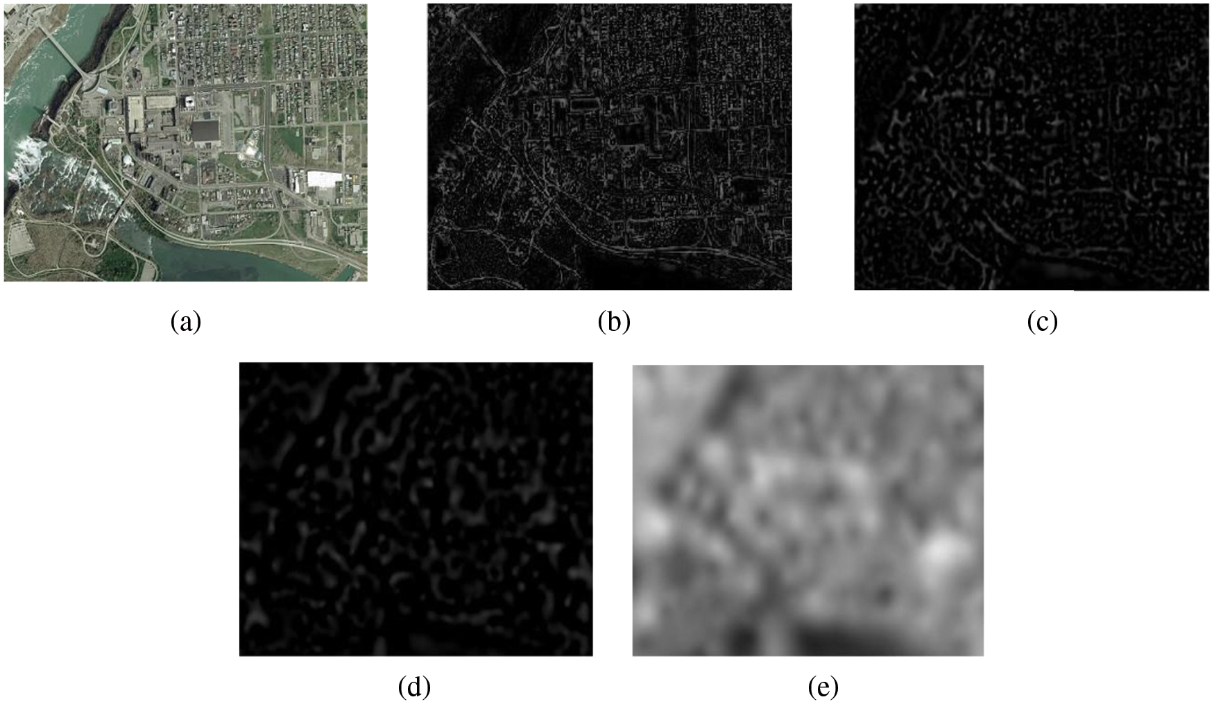
Figure 2: Image decomposition of SATELLITE VIEW image into IMF and residue (a) Original image (b) First IMF (c) Second IMF (d) Third IMF (e) Residue

Similarly, Fig. 3 represents various IMF and residue obtained of pool image by using sifting algorithm. It can be seen that first three IMF contains details present in an image and the residue contains lightness present.

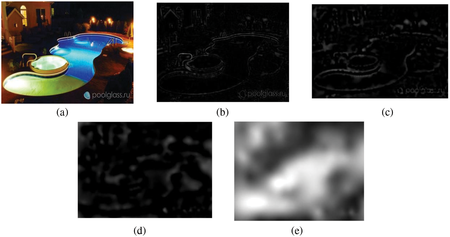
Figure 3: Image decomposition of POOL image into IMF and residue (a) Original image (b) First IMF (c) Second IMF (d) Third IMF (e) Residue

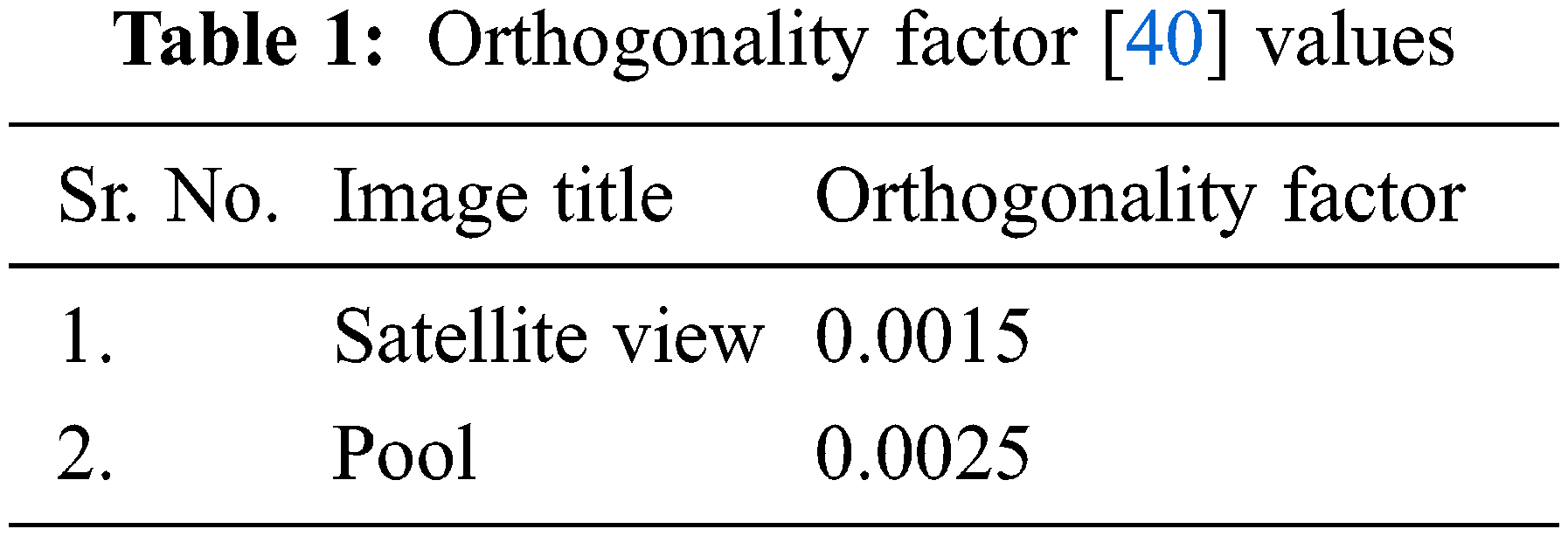
Tab. 1 represents the orthogonality factor values for different images. As discussed in Section 2, orthogonality factor value should be as low as possible for better decomposition of image into IMF and residue [40]. The orthogonality factor for satellite view and pool images are 0.0015 and 0.0025 these low values in Tab. 1 prove the decomposition process efficient one.

5  RBA based BEMD for Image Enhancement

The proposed algorithm, RBA based BEMD for enhancement of non-uniform illumination images, incorporates many stages for enhancement as shown in the block diagram in Fig. 4. The original non-uniform illumination color image is taken and conversion of RGB image into hue, saturation and intensity is done. Afterwards, the V transform is applied on the extracted intensity portion of the image. V transform has been discussed in Section 5.1 in details and BEMD is performed on the resulting V component to obtain the various bi-dimensional empirical modes and the residue as shown in Figs. 2 and 3. The linear transformation operations are performed on each BIMF separately and on the residue to enhance the details and lightness. The enhanced BIMFs and residue are combined together to get the final enhanced intensity component. Saturation component of HSV is enhanced in accordance to the enhanced V component as discussed in Section 5.3. Finally, hue, enhanced saturation and enhanced intensity component are added and converted to RGB domain to get final output enhanced image.

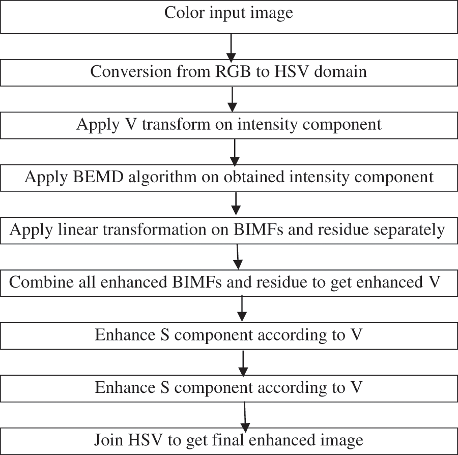
Figure 4: Block diagram of RBA based BEMD for enhancement of non-uniform illumination image

The non-uniform illumination image can be enhanced at a better level and the information that was not visible earlier in the original image can be seen effectively in the resultant image by using the proposed algorithm. Various techniques used during the algorithm have been discussed in the following subsections.

5.1 V Transform

The V transform consists of the brightness information of an image. Generally, many enhancement algorithms are used for enhancement of non-uniform illumination images like histogram equalization. Although, histogram equalization will increase the brightness of the image but changes the color of the original image too by increasing the contrast of the image. To preserve the natural colour of image, V transform is used. In the V transform, the given image is enhanced piece-wise. The given image is divided into number of small intervals and low intensity values are enhanced according to the highest value present in that particular interval. In this technique, the whole image is not enhanced uniformly but it has been enhanced as per the intensity value present locally in selected interval.

5.2 Linear Transformation

The linear transformations are the operations which are applied linearly on the given vectors of same dimension. These transformations basically require addition and scaling transformation on same dimension vector. The addition and scaling linear transformations is described by the following equation:

T(S1+S2)=T(S1)+T(S2) (13)

‘T(αS1)=αT(S1) (14)

In the proposed technique, linear operation has been applied on respective BIMFs and the residue for the enhancement purposes. The linear transformation operation is expressed by the given equation:

x∧v=∑i=1K(TiXfi)+Tk+1Xrk (15)

where Ti is transformation applied on BIMF and residue, x^v is enhanced V component after linear transformation, fi represents various BIMF and rk represents residue [41,42]. The transformation used for all BIMFs are the optimal weights to be multiplied by each component along with residue and further, on summation of all BEMD components, enhanced V image is obtained.

5.3 Saturation Component Enhancement

The saturation component of HSV domain is enhanced in accordance to the enhanced V component. First, ratio of enhanced V and original V is calculated and represented by γ (x, y) as shown below:

Γ(x,y)=x∧vxv (16)

where, x∧v and xv are enhanced and original intensity component.

X∧s(x,y)={γβ(x,y)xs(x,y),ifγ(x,y)>1xs(x,y),Otherwise (17)

where, x∧s(x,y) and xs(x,y) are the enhanced and original saturation components and β is constant used for determination of amount of enhancement for S component [43]. From the above expression, it can be concluded that if ratio of enhanced intensity to original intensity is higher than one, then original saturation component is enhanced by a factor power to ratio and if any other value occurs, then the enhanced saturation component value will be same.

After the enhancement of S and V components, H, S, V is combined to get final enhanced HSV image. At the end, HSV domain of image is converted into RGB domain.

6  Experimental Results and Discussion

6.1 Subjective Assessment

In this paper, proposed algorithm performance is compared with SSR, MSRCR, DCT based enhancement and JND based enhancement algorithm. Fig. 5a represents the original image of a bird which is captured under non-uniform illumination condition so the details of background are not visible properly. Fig. 5b represents the enhanced image using SSR algorithm. The details of background are visible but color content of image has faded which degrades the performance. Fig. 5c represents the enhanced image using MSRCR algorithm. This algorithm provides enhanced image by restoring the colors present present in image and thus provides more visually pleasant image. Figs. 5d and 5e represents the DCT based enhancement and JND based enhancement which also provides comparable results. Fig. 5f represents the enhancement results of proposed algorithm. The enhanced image obtained by the proposed algorithm is the most visually pleasant image. The naturalness of image has also been preserved here.

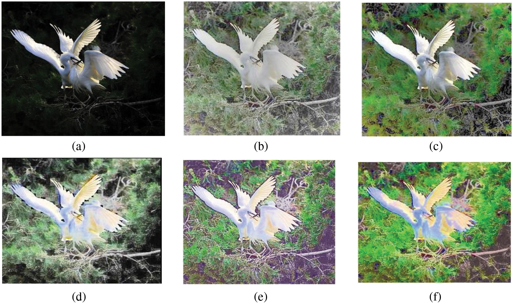
Figure 5: Comparative analysis of proposed algorithm with existing algorithms for a BIRD image (a) Original image (b) SSR (c) MSRCR (d) DCT (e) JND (f) Proposed algorithm

Fig. 6a represents the original image and Figs. 6 b and 6c represents the enhanced image using SSR and MSRCR algorithms in which SSR is performed by taking surround function value 15 and MSRCR by taking 15, 80, 255 as surround values. It can be seen that color restoration algorithm is doing well in preserving the color of image as the red color near the edge of the table is visible now more gracefully.

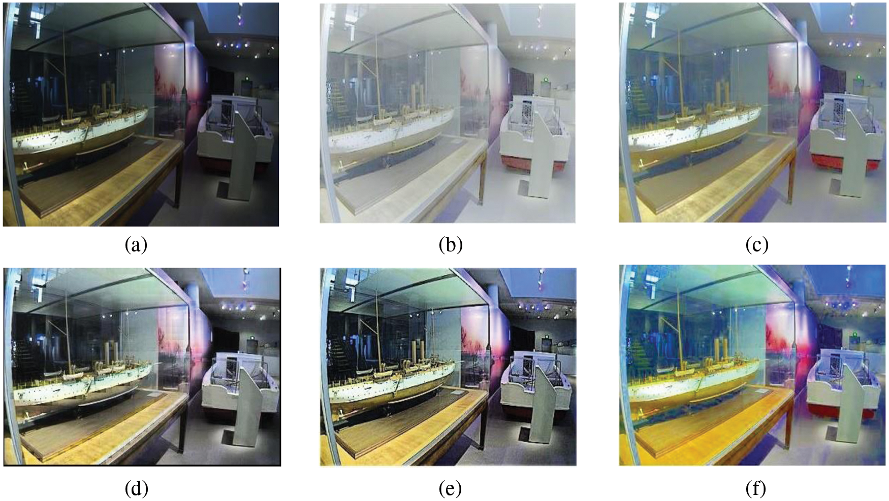
Figure 6: Comparative analysis of proposed algorithm with existing algorithms for a SHIP image (a) Original image (b) SSR (c) MSRCR (d) DCT (e) JND (f) Proposed algorithm

Fig. 6d represents the enhanced image by scaling DCT coefficients which enhance the information hidden in original image to a certain level but it gives a bit blurry output image as during processing blocking artifacts occurs. Fig. 6e represents the enhanced image by JND based algorithm. The image which was dark earlier is now bright image but this algorithm is not table to extract all the information as the true colors present in the image are not visible in the enhanced image.

Fig. 6f represents the image enhanced by using RBA based BEMD for enhancement which is proposed algorithm and gives the best results amongst all used algorithms. In fact, subjective and objective both evaluations can be done on the enhanced image by proposed technique very easily. Similarly, Figs. 7f and 8f gives the enhanced results of satellite view and house images by using proposed algorithm. It can be seen that all of these images give most visually pleasant results which are rich in details too by proposed algorithm in comparison to other mentioned enhancement algorithms.

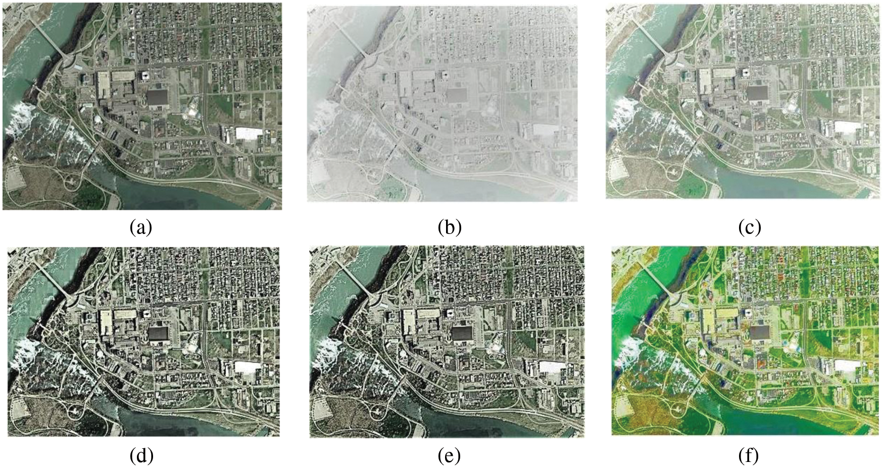
Figure 7: Comparative analysis of proposed algorithm with existing algorithms for a SATELLITE VIEW image (a) Original image (b) SSR (c) MSRCR (d) DCT (e) JND (f) Proposed algorithm

Figure 8: Comparative analysis of proposed algorithm with existing algorithms for a HOUSE image (a) Original image (b) SSR (c) MSRCR (d) DCT (e) JND (f) Proposed algorithm

6.2 Objective Assessment

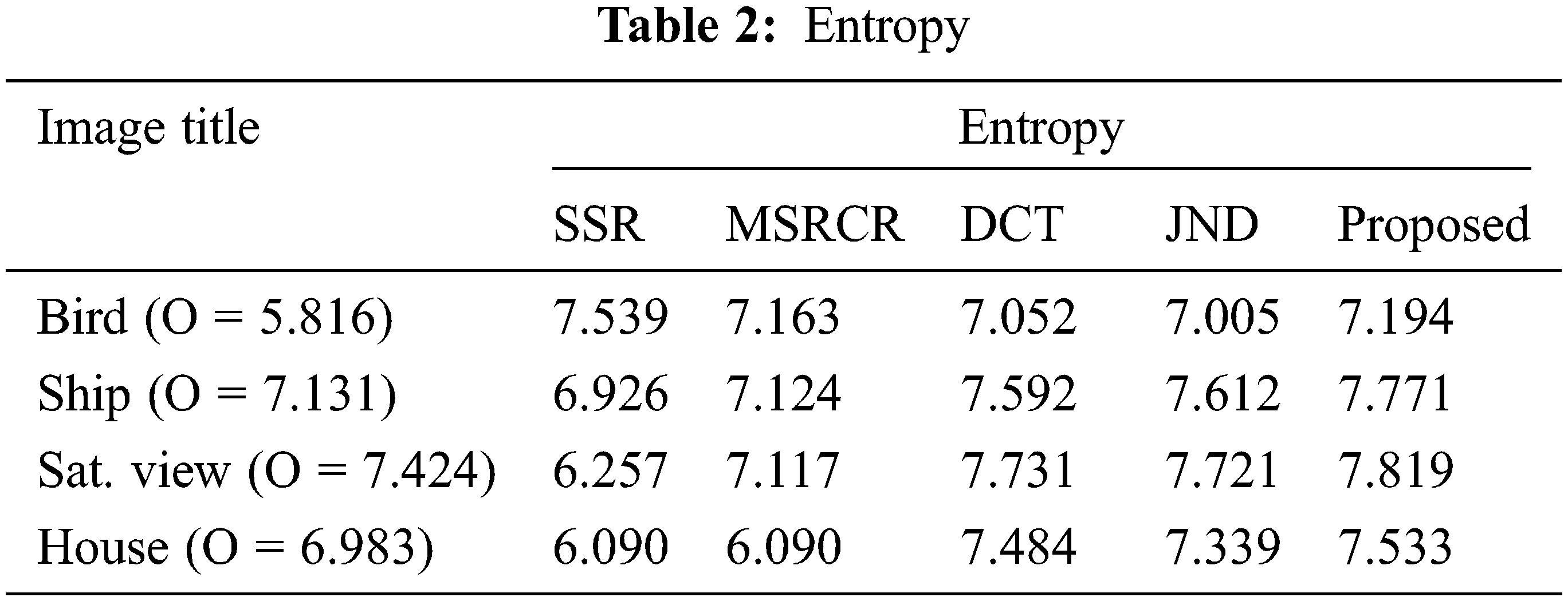
The image quality metric used are entropy and CQE (Color Quality Enhancement). Tabs. 2 and 3 represents the comparative performance of existing algorithms with proposed algorithm on basis of entropy and CQE. First quality metric is entropy. The second order performance measures can be used for determining the pixel variations in an image which is based on the grey level co-occurrence matrix. Entropy is one of those performance measures. It is expressed as follows:

Entropy=−∑i∑jO(i,j)log⁡O(i,j) (18)

where, O(i,j) is the grey level co-occurrence matrix. Higher the value of entropy, richer the image will be in context of details [44]. The second image quality metric is CQE. It is a quality measure that will combine the color information of image along with contrast and sharpness by multiplying each component with optimal weights. CQE can be expressed as follows:

CQE=c1×colorfulness+c2×sharpness+c3×contrast (19)

Colorfulness=0.02Xlog⁡σp2|μp|0.2Xlog⁡σσ2|μσ|0.2 (20)

where, σp2 and σσ2 are variance of color opponent axes, p and σ are opponent red-green and blue yellow components. Greater value of colorfulness represents the more enhanced image.

Sharpness=∑k=13akEME(grayedge) (21)

EME=2s1s2∑l=1s1∑k=1s2logLmax,k,1Lmin,k,1 (22)

where, ak are weights of various color components, Lmax,k,1 and Lmin,k,1 are maximum and minimum value in each block.

Contrast=AMEcontrast(V) (23)

AMEContrast=2s1s2∑l=1s1∑k=1s2(log⁡Lmax,k,1+Lmin,k,1Lmax,k,1−Lmin,k,1)−0.5 (24)

where, V is intensity of input color image [45].

Tab. 2 gives comparative analysis of different type of images using SSR, MSRCR, DCT based enhancement, JND based enhancement and proposed algorithm based on entropy parameter. From Tab. 2, the entropy of original bird image is 5.816 and the entropy obtained by SSR, MSRCR, DCT, JND and proposed algorithm are 7.163, 7.052, 7.005 and 7.194. Similarity, entropy values obtained from different images are shown in Tab. 2.

The performance comparison of all existing algorithms discussed in this paper with proposed algorithm on bias of CQE quality metric is shown in Tab. 3. From Tab. 3, the CQE value of bird image using SSR, MSRCR, DCT, JND and proposed algorithm are 0.4865, 0.4908, 0.5343, 0.5921 and 0.7493. It is observed from the table that CQE value in most of the images is lowest for single scale Retinex and highest for proposed enhancement algorithm. Image named as House has high value of CQE for JND based algorithm relative to proposed enhancement algorithm. It is due to the fact that sometimes the parameter value depends on type of image is to be taken. It can be observed from Tab. 3 that the proposed enhancement algorithm will gives the highest value of color quality enhancement metric most of the times for any type of image is to be taken as input.

7  Conclusions

The proposed algorithm enhances the non-uniform illumination images while preserving the naturalness and the information content of image. Enhancement algorithm is applied in HSV domain of image where intensity and saturation parts are being enhanced. The process starts by decomposing the intensity into various high and low frequency intrinsic mode functions and then apply linear transformations on them. The enhancement of saturation part is being done in accordance to enhanced intensity component, makes it more efficient algorithm. The subjective and objective assessment shows that the proposed algorithm provides better results as compare to various state of art methods for non-uniform illumination image enhancement.

Acknowledgement: The authors are grateful to Indraprastha Engineering College, Ghaziabad, India, ABES Institute of Technology, Ghaziabad, India and King Khalid University, Abha, Saudi Arabia for their permission and support to publish the research.

Funding Statement: This research is financially supported by the Deanship of Scientific Research at King Khalid University under research grant number (R.G.P 2/157/43).

Conflicts of Interest: The authors declare that they have no conflicts of interest to report regarding the present study.

References

1. Bovik, Image and video processing. New York, USA: Academics, 2000. [Google Scholar]
2. R. Gonzalez and R. Woods, Digital image processing. In: Pearson International Edition, 3rd ed., vol. 1. New Jersey, USA: Prentice-Hall, pp. 1–962, 2008. [Google Scholar]
3. H. Sawant and M. Deore, “A comprehensive review of image enhancement techniques,” Journal of Computing, vol. 2, no. 3, pp. 39–44, 2010. [Google Scholar]
4. A. Vishwakarma and A. Mishra, “Color image enhancement techniques: A critical review,” Indian Journal of Computer Science and Engineering, vol. 3, no. 1, pp. 2033–2044, 2012. [Google Scholar]
5. S. Rahman, M. M. Rahman, K. Hussain, S. M. Khaled and M. Shoyaib, “Image enhancement in spatial domain: A comprehensive study,” in 2014 17th Int. Conf. on Computer and Information Technology (ICCIT), Dhaka, Bangladesh, pp. 22–23, 2014. [Google Scholar]
6. S. Chaudhary, S. Raw, A. Biswas and A. Gautam, “An integrated approach of logarithmic transformation and histogram equalization for image enhancement,” in Proc. of 4th Int. Conf. on Soft Computing for Problem Solving, in Advances in Intelligent Systems and Computing 335, India, pp. 59–70, 2014. [Google Scholar]
7. S. Rahman, M. M. Rahman, M. A. Wadud, G. D. Quaden and M. Shoyaib, “An adaptive gamma correction for image enhancement,” EURASIP Journal of Image and Video Processing, vol. 2016, no. 1, pp. 1814, 2016. [Google Scholar]
8. R. Dorothy, R. Joany, R. J. Rathish, S. S. Prabha and S. Rajendran, “Image enhancement by Histogram equalization,” International Journal of Nano Corrosion Science and Engineering, vol. 2, no. 4, pp. 21–30, 2015. [Google Scholar]
9. A. M. Grigoryan, A. John and S. S. Agaian, “Alpha rooting Color Image Enhancement Method by Two-Side 2-D quaternion discrete Fourier transform followed by spatial transformation,” International Journal of Applied Control, Electrical and Electronics Engineering (IJACEEE), vol. 6, no. 1, pp. 1–21, 2018. [Google Scholar]
10. A. Hurlbert, “The computation of color,” Ph.D. dissertation, MIT, Cambridge, 1989. [Google Scholar]
11. B. Funt, F. Ciurea and J. J. McCann, “Retinex in Matlab,” Journal of Electronic Imaging, vol. 13, no. 1, pp. 48–57, 2004. [Google Scholar]
12. S. Wang and Y. Geng, “Image enhancement based on Retinex and lightness decomposition,” in Proc. of. 2011 18th IEEE Int. Conf. on Image Processing, Brussels, Belgium, pp. 3417–3420, 2011. [Google Scholar]
13. D. Jobson and Z. Rahman, “Properties and performance of a centre/surround Retinex,” IEEE Transaction on Image Processing, vol. 6, no. 3, pp. 451–462, 1997. [Google Scholar]
14. Z. Rahman, D. J. Jobson and G. A. Woodell, “Retinex processing for automatic image enhancement,” Journal of Electronic Imaging, vol. 13, no. 1, pp. 100–110, 2004. [Google Scholar]
15. D. J. Jobson and Z. Rahman, “A multi scale Retinex for bridging the gap between color images and the human observation of scenes,” IEEE Transaction on Image Processing, vol. 6, no. 3, pp. 965–976, 1997. [Google Scholar]
16. J. Mukherjee and S. Mitra, “Enhancement of color images by scaling the DCT coefficients,” IEEE Transaction on Image Processing, vol. 17, no. 10, pp. 1783–1794, 2008. [Google Scholar]
17. W. A. Mustafa, H. Yazid, W. Khairunizam, M. A. Jamlos, I. Zunaidi et al., “Image enhancement based on discrete cosine transforms (DCT) and discrete wavelet transform (DWTA review,” in IOP Conf. Series.: Material Science and Engineering 557, Bogor, Indonesia, 2019. [Google Scholar]
18. L. Wang, G. Fu, Z. Jiang, G. Ju and A. Men, “‘Low-light image enhancement with attention and multi-level feature fusion,” in Proc. of. IEEE Int. Conf. on Multimedia and Expo Workshops (ICMEW), Shanghai, China, pp. 276–281, 2019. [Google Scholar]
19. A. Toet, M. A. Hogervorst, R. van Son and J. Dijk, “Augmenting full colour-fused multi-band night vision imagery with synthetic imagery in real-time,” International Journal on Image Data Fusion, vol. 2, no. 4, pp. 287–308, 2011. [Google Scholar]
20. D. Choi, I. H. Jang, M. H. Kim and N. C. Kim, “Color image enhancement using single-scale retinex based on an improved image formation model,” in 16th European Conf. on Signal Processing, Lausanne, Switzerland, pp. 25–29, 2008. [Google Scholar]
21. S. A. Rajala, M. R. Civanlar and W. M. Lee, “A second generation image coding technique using human visual system-based segmentation,” in Proc. of IEEE Int. Conf. on Acoustics, Speech, and Signal Processing, Dallas, TX, vol. 12, pp. 1362–1365, 1987. [Google Scholar]
22. H. Xia and M. Liu, “Non uniform illumination image enhancement based on Retinex and gamma correction,” in IOP Conf. Series: Journal of Physics: Conf. Series 1213, pp. 052072, 2019. [Google Scholar]
23. G. W. Griffiths and W. E. Schiesser, “Linear and nonlinear waves,” Scholarpedia, vol. 4, no. 7, pp. 1–35, 2011. [Google Scholar]
24. V. Puliafito, S. Vergura and M. Carpentieri, “Fourier, Wavelet and Hilbert Huang transforms for studying electrical users in the time and frequency domain,” Energies, vol. 10, no. 2, pp. 1–14, 2017. [Google Scholar]
25. R. Senthilkumar, A. Romolo, V. Fiamma, F. Arena and K. Murali, “Analysis of wave groups in crossing seas using hilbert huang transformation,” Procedia Engineering, vol. 116, no. 3, pp. 1042–1049, 2015. [Google Scholar]
26. V. D. Ompokov and V. V. Boroneov, “Mode decomposition and the hilbert huang transform,” in 2019 Russian Open Conf. on Radio Wave Propagation (RWP), Kazan, Russia, 2019. [Google Scholar]
27. A. Zeiler, R. Faltermeier, I. R. Keck, A. M. Tomé, G. C. Puntonet et al., “Empirical mode decomposition-an introduction,” in IEEE Int. Joint Conf. on Neural Networks, Barcelona, Spain, 2010. [Google Scholar]
28. A. Stallone, A. Cicone and M. Materassi, “New insights and best practices for the successful use of Empirical Mode Decomposition, iterative filtering and derived algorithms,” Scientific Reports-Nature, vol. 10, no. 15161, pp. 243, 2020. [Google Scholar]
29. R. Fontugne, P. Borgnat and P. Flandrin, “Online empirical mode decomposition,” in 2017 IEEE Int. Conf. on Acoustic, Speech and Signal Processing (ICASSP), New Orleans, LA, USA, pp. 5–9, 2017. [Google Scholar]
30. Y. Washizawa, T. Tanaka, D. P. Mandic and A. Cichocki, “A flexible method for envelope estimation in empirical mode decomposition,” in Proc. of Int. Conf. on Knowledge Based Intelligent Information and Engineering Systems, Bournemouth, UK, pp. 1248–1255, 2006. [Google Scholar]
31. N. E. Huang, Z. Shen, S. R. Long, M. C. Wu, H. H. Shih et al., “The empirical mode decomposition and the Hilbert spectrum for nonlinear and non-stationary time series analysis,” in Proc. of Royal Society: A Mathematical, Physical and Engineering Science, London, pp. 903–995, 1998. [Google Scholar]
32. M. C. Peel, G. G. S. Pegram and T. A. McMahon, “Empirical mode decomposition: improvement and application,” in Proc. of Int. Congress on Modelling Simulation, Canberra, Modelling and Simulation Society of Australia, pp. 2996–3002, 2007. [Google Scholar]
33. M. Smolik and V. Skala, “Large scattered data interpolation with radial basis functions and space subdivisions,” Integrated Computer Aided Engineering, vol. 25, no. 1, pp. 49–62, 2017. [Google Scholar]
34. M. Tatari, “A localized interpolation method using radial basis functions,” International Journal of Mathematics and Computer Science, vol. 4, no. 9, pp. 1281–1286, 2010. [Google Scholar]
35. B. S. Morse, T. S. Yoo, P. Rheingans, D. T. Chen and K. R. Subramanian, “Interpolating implicit surfaces from scattered surface data using compactly supported radial basis functions,” in Proc. of Int. Conf. on Shape Modelling Applications, Genova, Italy, pp. 89–98, 2001. [Google Scholar]
36. Y. Ding, “Multiset canonical correlations analysis of bidimensional intrinsic mode functions for automatic target recognition of SAR images,” Computational Intelligence and Neuroscience, vol. 2021, no. 2, pp. 1–13, 2021. [Google Scholar]
37. C. Wang, Q. Kemao and F. Da, “Automatic fringe enhancement with novel bidimensional sinusoids-assisted empirical mode decomposition,” Optics Express, vol. 25, no. 20, pp. 24299–24311, 2017. [Google Scholar]
38. P. M. Palkar, V. R. Udupi and S. A. Patil, “A review on bidimensional empirical mode decomposition: A novel strategy for image decomposition,” in 2017 Int. Conf. on Energy, Communication, Data Analytics and Soft Computing (ICECDS), Chennai, India, pp. 1–2, 2017. [Google Scholar]
39. Z. Yang, J. Jiang, L. Yang, C. Qing, B. W. Ling et al., “A new bidimensional EMD algorithm and its applications,” in 2014 9th Int. Symp. on Communication System, Network Digital Sign (CSNDSP), Manchester, UK, 2014. [Google Scholar]
40. S. M. Bhuiyan, J. F. Khan and R. R. Adhami, A bi-dimensional empirical mode decomposition method for color image processing. In: IEEE Workshop on Signal Processing and Systems. San Francisco, CA, pp. 272–277, 2010. [Google Scholar]
41. M. Zhang, F. Zou and J. Zheng, “The linear transformation image enhancement algorithm based on HSV color space,” in Proc. of 12th Int. Conf. on Intelligent Information Hiding and Multimedia Signal Processing, Kaohsiung, Taiwan, vol. 2, pp. 19–27, 2017. [Google Scholar]
42. P. Janani, J. Premalatha and K. S. Ravichandaran, “Image enhancement techniques: A study,” Indian Journal of Science and Technology, vol. 8, no. 22, pp. 1–12, 2015. [Google Scholar]
43. D. Choi and I. Jang, “Color image enhancement based on single-scale Retinex with a JND based nonlinear filter,” in IEEE Int. Symp. on Circuits and Systems, New Orleans, LA, pp. 3948–3951, 2007. [Google Scholar]
44. T. Samajdar and M. Quraishi, “Analysis and evaluation of image quality metrics,” in Proc. of 2nd Int. Conf. on Information Systems Design and Intelligent Applications, India, vol. 340, pp. 369–378, 2015. [Google Scholar]
45. A. M. Eskicioglu and P. Fisher, “Image quality measures and their performance,” IEEE Transaction on Communication, vol. 43, no. 12, pp. 2959–2965, 1995. [Google Scholar]
Cite This Article
Copyright © 2023 The Author(s). Published by Tech Science Press.
This work is licensed under a Creative Commons Attribution 4.0 International License , which permits unrestricted use, distribution, and reproduction in any medium, provided the original work is properly cited.
Downloads
Citation Tools