
 Submit a Paper
 Propose a Special lssue
 Open Access
ARTICLE
WACPN: A Neural Network for Pneumonia Diagnosis
1 School of Computing and Mathematical Sciences, University of Leicester, Leicester, LE1 7RH, UK
2 Department of Computer Science, HITEC University Taxila, Taxila, Pakistan
* Corresponding Author: Yu-Dong Zhang. Email:
Computer Systems Science and Engineering 2023, 45(1), 21-34. https://doi.org/10.32604/csse.2023.031330
Received 14 April 2022; Accepted 17 May 2022; Issue published 16 August 2022
 View Full Text
 Download PDF
Abstract
Community-acquired pneumonia (CAP) is considered a sort of pneumonia developed outside hospitals and clinics. To diagnose community-acquired pneumonia (CAP) more efficiently, we proposed a novel neural network model. We introduce the 2-dimensional wavelet entropy (2d-WE) layer and an adaptive chaotic particle swarm optimization (ACP) algorithm to train the feed-forward neural network. The ACP uses adaptive inertia weight factor (AIWF) and Rossler attractor (RA) to improve the performance of standard particle swarm optimization. The final combined model is named WE-layer ACP-based network (WACPN), which attains a sensitivity of 91.87 ± 1.37%, a specificity of 90.70 ± 1.19%, a precision of 91.01 ± 1.12%, an accuracy of 91.29 ± 1.09%, F1 score of 91.43 ± 1.09%, an MCC of 82.59 ± 2.19%, and an FMI of 91.44 ± 1.09%. The AUC of this WACPN model is 0.9577. We find that the maximum deposition level chosen as four can obtain the best result. Experiments demonstrate the effectiveness of both AIWF and RA. Finally, this proposed WACPN is efficient in diagnosing CAP and superior to six state-of-the-art models. Our model will be distributed to the cloud computing environment.Keywords
Community-acquired pneumonia (CAP) is considered a sort of pneumonia [1] developed outside hospitals, and clinics, along with infirmaries [2]. CAP may affect people of any age, but it is more prevalent in very young and elderly groups, which may need hospital treatment if they develop CAP [3]. Chest computed tomography (CCT) is a crucial way to help radiologists/physicians to diagnose CAP patients. Recently, automatic diagnosis models based on artificial intelligence (AI) have gained promising performances and attracted researchers’ attention. For example, Heckerling, et al. [4] employed the genetic algorithm for neural networks to foresee CAP. This approach is shortened to the genetic algorithm for pneumonia (GAN). Afterward, Liu, et al. [5] proposed a computer-aided detection (CADe) model to uncover lung nodules in the CCT slides. Strehlitz, et al. [6] presented several prediction systems by means of support vector machines (SVMs) together with Monte Carlo cross-validation. Dong, et al. [7] proposed an improved quantum neural network (IQNN) for pneumonia image recognition. Ishimaru, et al. [8] proposed a decision tree (DT) model to foresee the atypical pathogens of CAP. Zhou [9] introduced the cat swarm optimization (CSO) method to recognize CAP. Wang, et al. [10] proposed an advanced deep residual dense network for the image super-resolution problem. Wang, et al. [11] proposed a CFW-Net for X-ray based COVID-19 detection.
However, the above methods still have room to improve. Their recognition performances, for example, the accuracies, are no more than or barely above 91.0%. We analyze their models and believe the reason is their training algorithms. After comparing recent global optimization algorithms, we find that particle swarm optimization (PSO) is one of the most successful optimization algorithms, compared to otheroptimization algorithms such as artificial bee colony [12] and bat algorithm [13]. Hence, we use the framework in Zhou [9] but replace CSO with an improved PSO. In addition, we introduce the two-dimensional wavelet-entropy (2d-WE) layer, introduce an improved PSO method—adaptive chaotic PSO (ACP) [14], and combine it with a feed-forward neural network. The final combined model is named WE-layer ACP-based network (WACPN). The experiments show the effectiveness of this proposed WACPN model. In all, we exhibit three contributions:
(a) The 2d-WE layer is managed as the feature extractor.
(b) ACP is utilized for training the neural network to gain a robust classifier.
(c) The proposed WACPN is proven to give better results than six state-of-the-art models.
The dataset is described in Zhou [9], where we have 305 CAP images and 298 healthy control (HC) images. The detailed demographical information can be found in Ref. [9]. Assume the raw CCT dataset is signified as
where
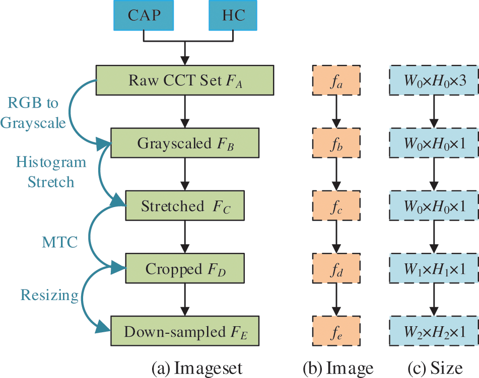
Figure 1: Diagram of preprocessing
Initially, the color CCT image set
Second, we use histogram stretching (HS) on all images
where
Third, margin & text cropping (MTC) is implemented to eradicate (a) the checkup bed at the bottom zone, (b) the privacy-related scripts at the margin or corner zones, and (c) the ruler adjacent to the right-side and bottom zones. The MTCed image set
Lastly, each image in
Fig. 1c shows the extent of every raw image in
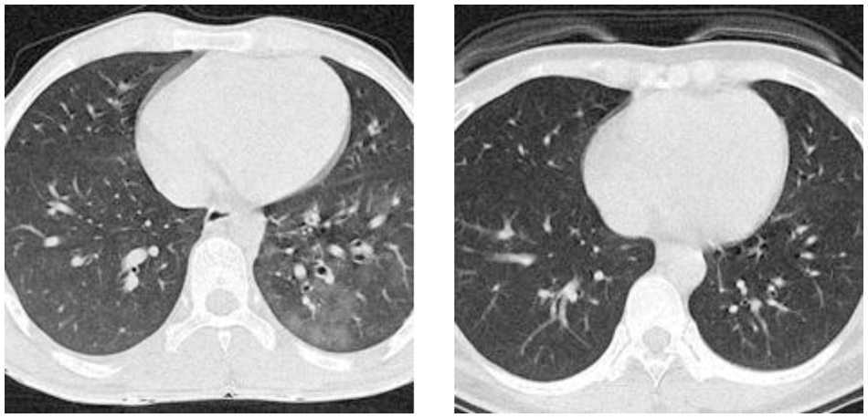
Figure 2: Examples of the preprocessed image set
3.1 Discrete Wavelet Transform
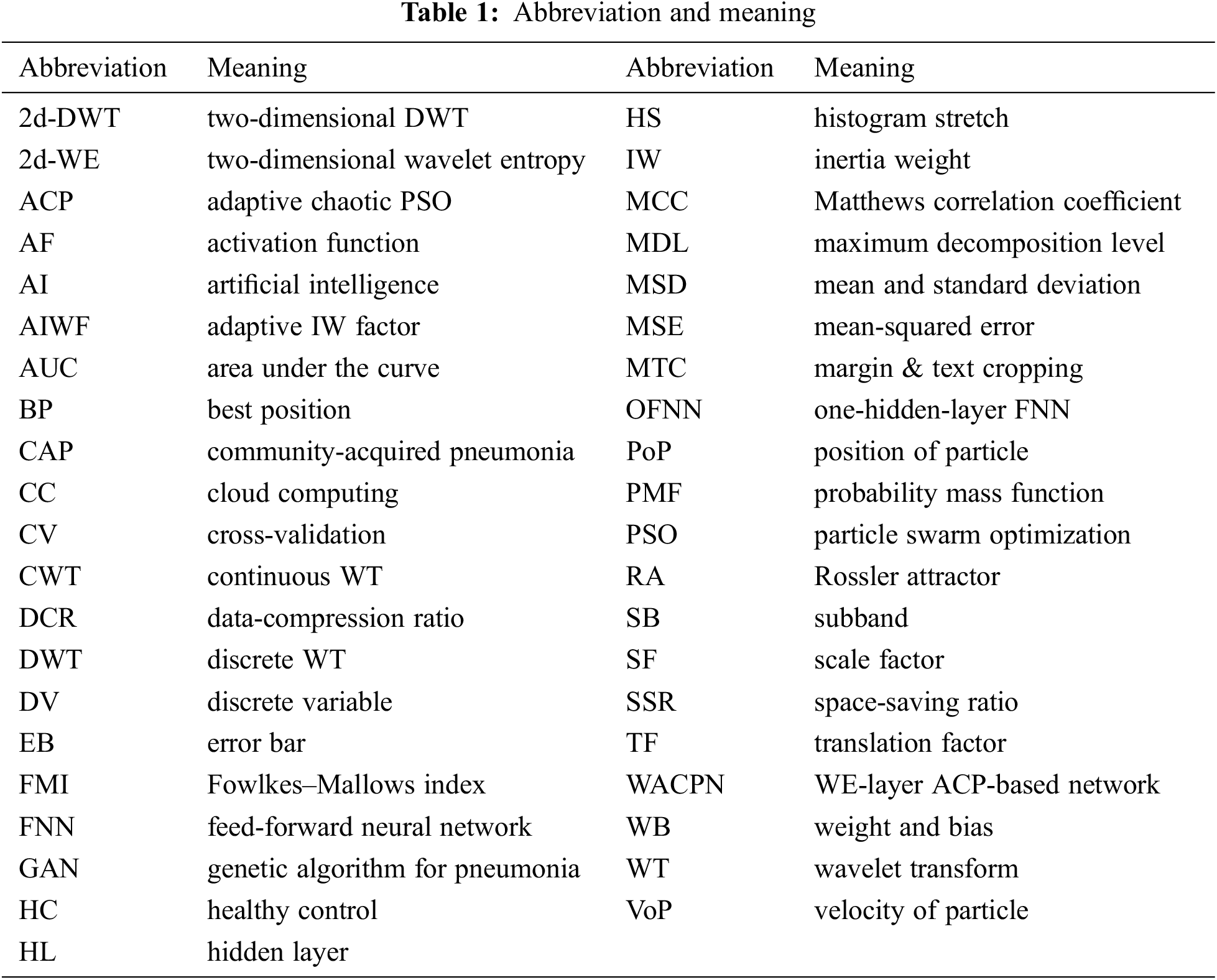
Tab. 1 enumerates all abbreviations and their associated meanings. The advantage of wavelet transform (WT) is that it holds both time/spatial and frequency information of the given signal/image. Nevertheless, the discrete wavelet transform (DWT) is chosen to convert the raw signal
in which E stands for the wavelet coefficient,
where the
Now, we deduct the definition of DWT from CWT. The Eq. (5) is discretized by substituting
where c signifies the DV of the SF
where
where
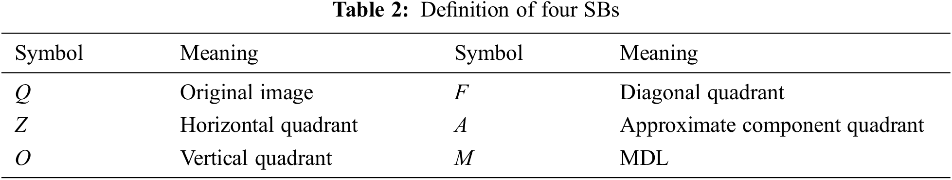
Suppose we handle a two-dimensional (2d) image Q; the 2d-DWT [17] is worked out by processing row-wise and column-wise 1d-DWT in succession [15]. Initially, the 2d-DWT operates on the original image Q. Later, four SBs
Assuming
The subsequent decompositions run as:
where M is the MDL and m the current decomposition level [18].
The subband
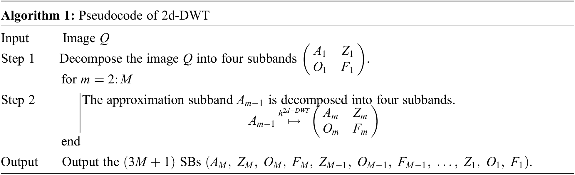
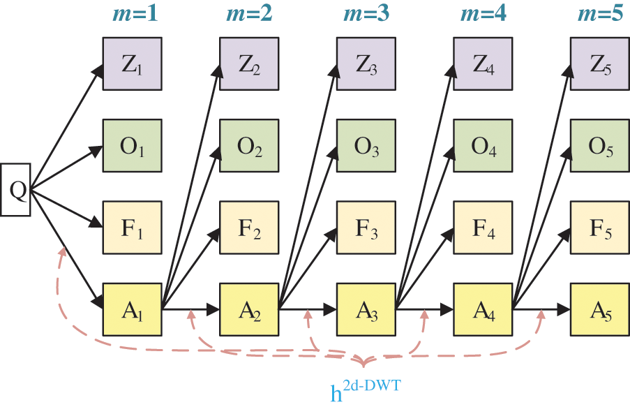
Figure 3: Diagram of a 2d-DWT
The
where
Second, the entropy of the PMF
where
Lastly, the entropy values of the whole SBs are concatenated to grow a feature vector I.
where the number of the features in I is
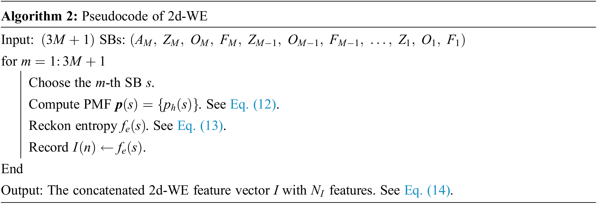
The
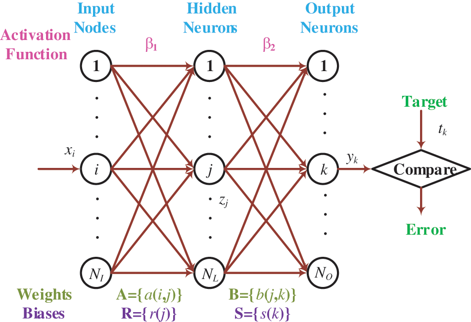
Figure 4: Diagram of an FNN
Assume
where
where
The parameter training is an optimization problem that guides us to search for the optimal WB parametric vector
Recap that two attributes (position x and velocity
The first is the BP a particle p has traversed till now. It is dubbed pBest and symbolized as
If p takes the entire swarm as its neighborhood, the nBest turns to the global best and is for that reason named gBest. In standard PSO, the VoP v of particle p is updated as:
where
where
The ACP algorithm proposed an adaptive IW factor (AIWF) strategy. It uses
Here,
Another improvement in ACP is upon the two random numbers
where
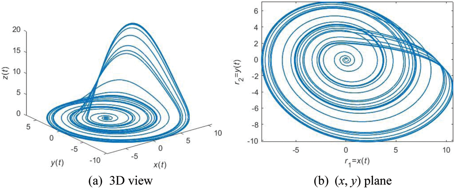
Figure 5: An example of RA with parameters of (δa = 0.2, δb = 0.4, δc = 5.7)
We agree4 Experiments, Results, and Discussions
Ten runs of 10-fold cross-validation are used to relate a reliable performance of our WACPN model. Besides, we use the following measures—sensitivity (Sen, symbolized as
The parameters of this study are listed in Tab. 3. The sizes of the original images are
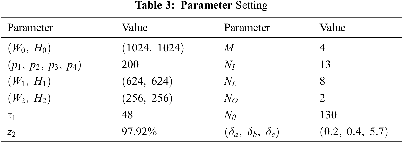
Fig. 6 shows the wavelet decomposition results with
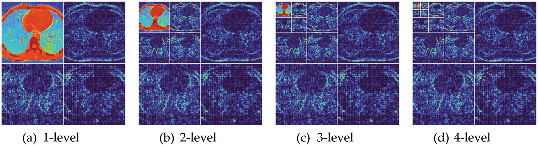
Figure 6: Wavelet decomposition results
4.3 Results of Proposed WACPN Model
Tab. 4 shows the ten runs of 10-fold CV via the parameters shown in Tab. 3, where
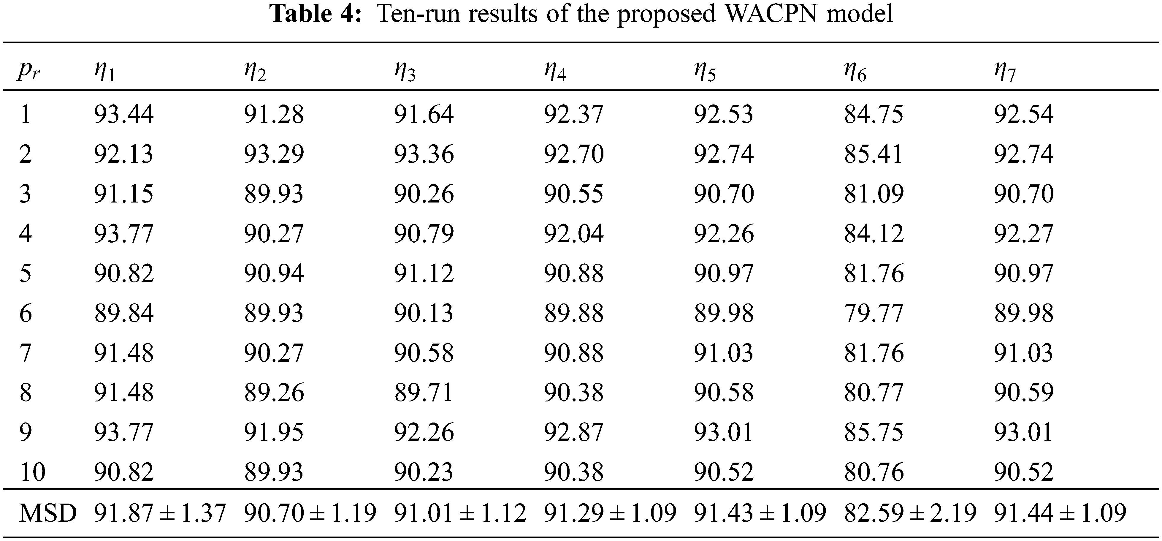
If we remove the AIWF from our WACPN model, the results using the same configuration are shown in Tab. 5. Similarly, the results of removing RA from our WACPN model are shown in Tab. 6. After comparing the results in Tab. 4 against the results in Tabs. 5 and 6, we can deduce that both strategies—AIWF and RA—are beneficial to our WACPN model.
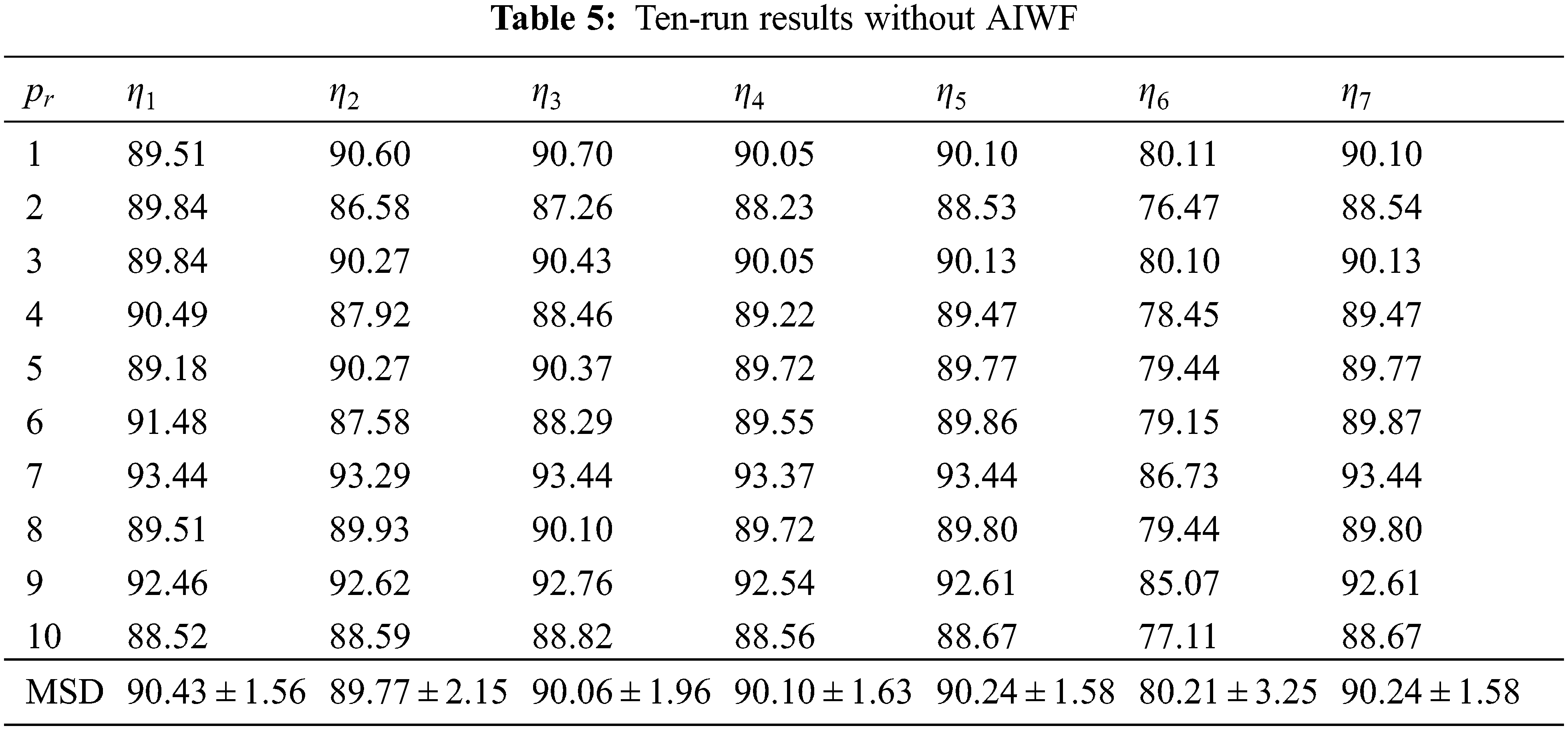
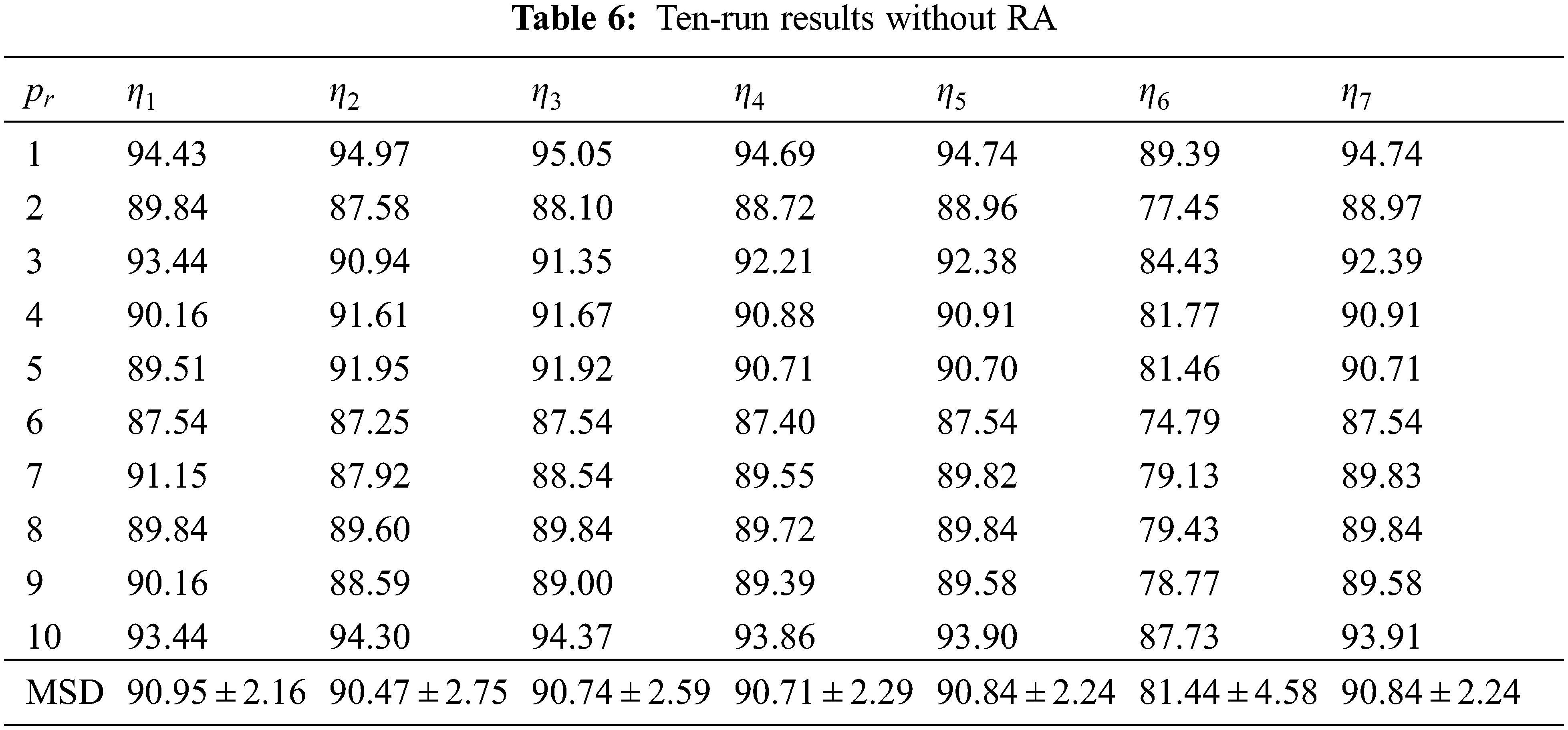
Fig. 7 represents the ROC curves together with their upper and lower bounds of the proposed WACPN model and its two ablation studies (without AIWF and without RA). The AUC of WACPN model is 0.9577. The AUCs of the models removing AIWF or RA are only 0.9319 and 0.9456, respectively, demonstrating that both AIWF and RA help improve the standard PSO.
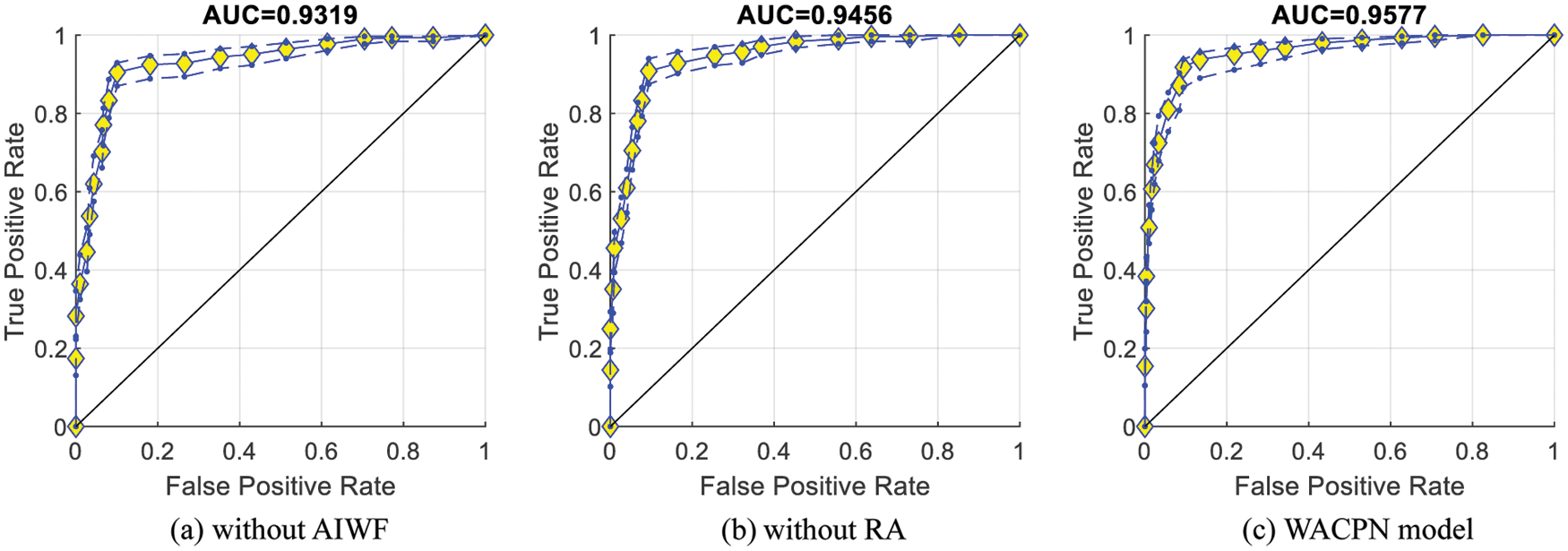
Figure 7: ROC curves
4.5 Comparison with State-of-the-Art Models
The proposed WACPN model is judged with six state-of-the-art models: GAN [4], CADe [5], SVM [6], IQNN [7], DT [8], and CSO [9]. The evaluation results on the same dataset via ten runs of 10-fold CV are listed in Tab. 7.
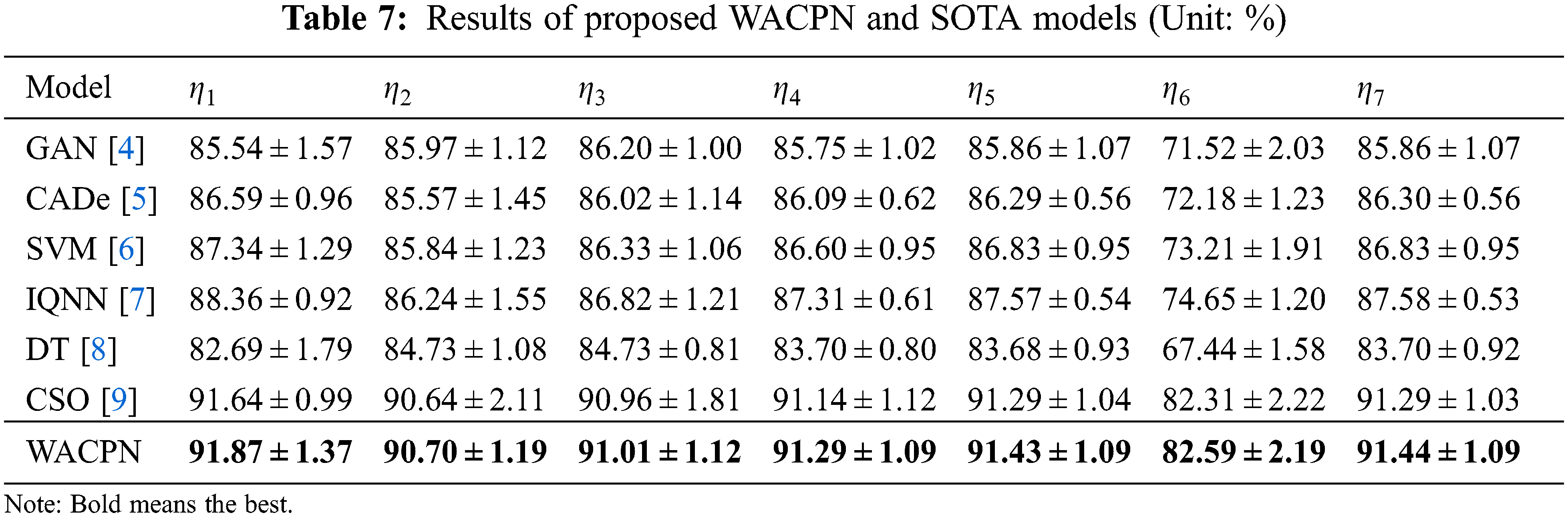
Error bar (EB) is an excellent tool for ease of visual evaluation. Fig. 8 presents the EB of model comparison, from which we can observe that the proposed WACPN model is superior to six state-of-the-art models. The causes are triple. First, the 2d-WE layer stands as a proficient way to designate CCT images. Second, ACP is efficient in training FNN. Third, we fine-tune and select the best parameters for the RA. In the future, our model may be applied to other fields [21,22].
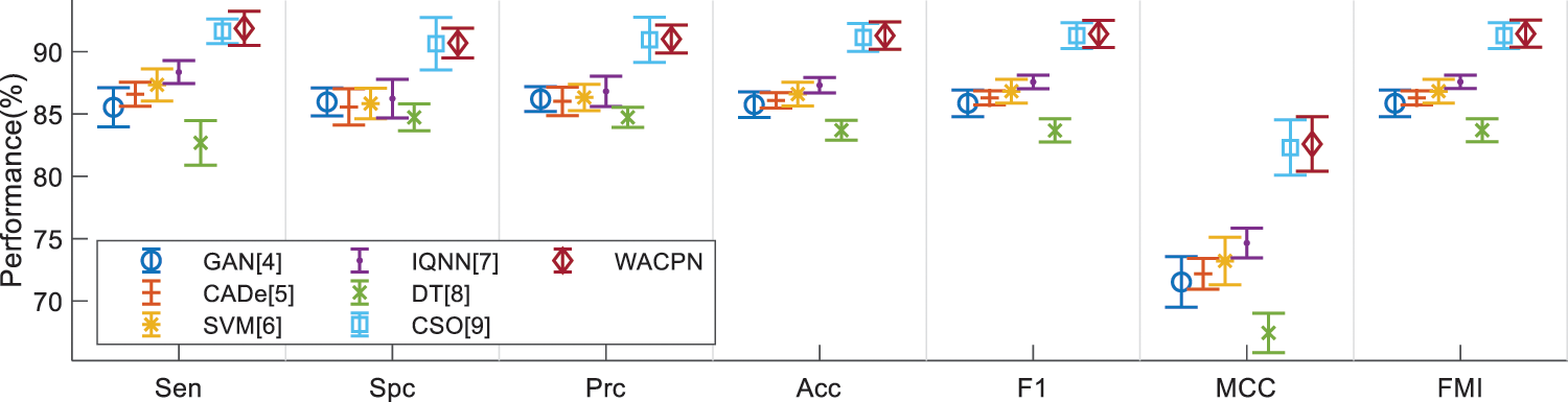
Figure 8: EB of model comparison
A novel WACPN method is proposed for diagnosing the CAP in CCT images. In WACPN, the 2d-WE layer works as feature extraction, and the optimization algorithm—ACP—is exercised to optimize the neural network. This proposed WACPN model is verified to have better results than six state-of-the-art models.
Three defects of the proposed WACPN model exist: (i) Deep learning models are not exercised. The reason is the small amount of our image set. (ii) Strict clinical validation is not tested either on-site or in cloud computing (CC) environments. (iii) The model is a black box, which does not go well with patients and doctors.
To work out the three limitations, first, we shall utilize the data augmentation method to enlarge the number of images in the dataset. Second, our team shall circulate the proposed WACPN model to the online CC environment (such as Azure) and summon specialists, clinicians, and physicians to examine its efficiency. Third, trustworthy or explainable Ais, which may provide the heatmaps pointing out the lesions, are two optional models to assist in adding explainability to the proposed WACPN model.
Funding Statement: This paper is partially supported by Medical Research Council Confidence in Concept Award, UK (MC_PC_17171); Royal Society International Exchanges Cost Share Award, UK (RP202G0230); British Heart Foundation Accelerator Award, UK (AA/18/3/34220); Hope Foundation for Cancer Research, UK (RM60G0680); Global Challenges Research Fund (GCRF), UK (P202PF11); Sino-UK Industrial Fund, UK (RP202G0289); LIAS Pioneering Partnerships award, UK (P202ED10); Data Science Enhancement Fund, UK (P202RE237).
Conflicts of Interest: The authors declare that they have no conflicts of interest to report regarding the present study.
References
1. G. Guarnieri, L. B. De Marchi, A. Marcon, S. Panunzi, V. Batani et al., “Relationship between hair shedding and systemic inflammation in covid-19 pneumonia,” Annals of Medicine, vol. 54, pp. 869–874, 2022. [Google Scholar]
2. J. E. Schneider and J. T. Cooper, “Cost impact analysis of novel host-response diagnostic for patients with community-acquired pneumonia in the emergency department,” Journal of Medical Economics, vol. 25, pp. 138–151, 2022. [Google Scholar]
3. M. T. Olsen, A. M. Dungu, C. K. Klarskov, A. K. Jensen, B. Lindegaard et al., “Glycemic variability assessed by continuous glucose monitoring in hospitalized patients with community-acquired pneumonia,” Bmc Pulmonary Medicine, vol. 22, Article ID: 83, 2022. [Google Scholar]
4. P. S. Heckerling, B. S. Gerber, T. G. Tape and R. S. Wigton, “Use of genetic algorithms for neural networks to predict community-acquired pneumonia,” Artificial Intelligence in Medicine, vol. 30, pp. 71–84, 2004. [Google Scholar]
5. X. L. Liu, F. Hou, H. Qin and A. M. Hao, “A cade system for nodule detection in thoracic ct images based on artificial neural network,” Science China-Information Sciences, vol. 60, pp. 15, Article ID: 072106, 2017. [Google Scholar]
6. A. Strehlitz, O. Goldmann, M. C. Pils, F. Pessler and E. Medina, “An interferon signature discriminates pneumococcal from staphylococcal pneumonia,” Frontiers in Immunology, vol. 9, Article ID: 1424, 2018. [Google Scholar]
7. Y. M. Dong, M. Q. Wu and J. L. Zhang, “Recognition of pneumonia image based on improved quantum neural network,” IEEE Access, vol. 8, pp. 224500–224512, 2020. [Google Scholar]
8. N. Ishimaru, S. Suzuki, T. Shimokawa, Y. Akashi, Y. Takeuchi et al., “Predicting mycoplasma pneumoniae and chlamydophila pneumoniae in community-acquired pneumonia (cap) pneumonia: Epidemiological study of respiratory tract infection using multiplex pcr assays,” Internal and Emergency Medicine, vol. 16, pp. 2129–2137, 2021. [Google Scholar]
9. J. Zhou, “Community-acquired pneumonia recognition by wavelet entropy and cat swarm optimization,” Mobile Networks and Applications, https://doi.org/10.1007/s11036-021-01897-0, 2022 (Online First). [Google Scholar]
10. W. Wang, Y. B. Jiang, Y. H. Luo, J. Li, X. Wang et al., “An advanced deep residual dense network (drdn) approach for image super-resolution,” International Journal of Computational Intelligence Systems, vol. 12, pp. 1592–1601, 2019. [Google Scholar]
11. W. Wang, H. Liu, J. Li, H. S. Nie and X. Wang, “Using cfw-net deep learning models for x-ray images to detect covid-19 patients,” International Journal of Computational Intelligence Systems, vol. 14, pp. 199–207, 2021. [Google Scholar]
12. K. Thirugnanasambandam, M. Rajeswari, D. Bhattacharyya and J. Y. Kim, “Directed artificial bee colony algorithm with revamped search strategy to solve global numerical optimization problems,” Automated Software Engineering, vol. 29, Article ID: 13, 2022. [Google Scholar]
13. W. Z. Al-Dyani, F. K. Ahmad and S. S. Kamaruddin, “Binary bat algorithm for text feature selection in news events detection model using markov clustering,” Cogent Engineering, vol. 9, Article ID: 2010923, 2022. [Google Scholar]
14. L. Wu, “Crop classification by forward neural network with adaptive chaotic particle swarm optimization,” Sensors, vol. 11, pp. 4721–4743, 2011. [Google Scholar]
15. M. Sahabuddin, M. F. Hassan, M. I. Tabash, M. A. Al-Omari, M. K. Alam et al., “Co-movement and causality dynamics linkages between conventional and islamic stock indexes in Bangladesh: A wavelet analysis,” Cogent Business & Management, vol. 9, Article ID: 2034233, 2022. [Google Scholar]
16. S. Kavitha, N. S. Bhuvaneswari, R. Senthilkumar and N. R. Shanker, “Magnetoresistance sensor-based rotor fault detection in induction motor using non-decimated wavelet and streaming data,” Automatika, vol. 63, pp. 525–541, 2022. [Google Scholar]
17. A. K. Gupta, C. Chakraborty and B. Gupta, “Secure transmission of eeg data using watermarking algorithm for the detection of epileptical seizures,” Traitement Du Signal, vol. 38, pp. 473–479, 2021. [Google Scholar]
18. A. Meenpal and S. Majumder, “Image content based secure reversible data hiding scheme using block scrambling and integer wavelet transform,” Sadhana-Academy Proceedings in Engineering Sciences, vol. 47, pp. 1–11, Article ID: 54, 2022. [Google Scholar]
19. O. Kammouh, M. W. A. Kok, M. Nogal, R. Binnekamp and A. R. M. Wolfert, “Mitc: Open-source software for construction project control and delay mitigation,” Softwarex, vol. 18, Article ID: 101023, 2022. [Google Scholar]
20. J. M. Malasoma and N. Malasoma, “Bistability and hidden attractors in the paradigmatic rossler'76 system,” Chaos, vol. 30, Article ID: 123144, 2020. [Google Scholar]
21. X. R. Zhang, X. Sun, W. Sun, T. Xu, P. P. Wang et al., “Deformation expression of soft tissue based on bp neural network,” Intelligent Automation and Soft Computing, vol. 32, pp. 1041–1053, 2022. [Google Scholar]
22. X. R. Zhang, X. Sun, X. M. Sun, W. Sun and S. K. Jha, “Robust reversible audio watermarking scheme for telemedicine and privacy protection,” Cmc-Computers Materials & Continua, vol. 71, pp. 3035–3050, 2022. [Google Scholar]
Cite This Article
 Copyright © 2023 The Author(s). Published by Tech Science Press.
This work is licensed under a Creative Commons Attribution 4.0 International License , which permits unrestricted use, distribution, and reproduction in any medium, provided the original work is properly cited.
 Downloads
 Citation Tools